Discrete representations of random signals

DOC.l..-;... ;' .DdCIfT ROOM 36-412 :R - a :. 'L 'i : -r.;C:' :,LCS

MAS~vv 'a ds' ''- t.' '_fi-A UC

_ __

21.

DISCRETE REPRESENTATIONS OF RANDOM SIGNALS

KENNETH L. JORDAN, JR.

L

TECHNICAL REPORT 378 JULY 14, 1961

C

S

MASSACHUSETTS INSTITUTE OF TECHNOLOGY

RESEARCH LABORATORY OF ELECTRONICS

CAMBRIDGE, MASSACHUSETTS

*3

O

cY\

The Research Laboratory of Electronics is an interdepartmental laboratory in which faculty members and graduate students from numerous academic departments conduct research.

The research reported in this document was made possible in part by support extended the Massachusetts Institute of Technology, Re-search Laboratory of Electronics, jointly by the U.S. Army (Signal Corps), the U.S. Navy (Office of Naval Research), and the U.S. Air Force (Office of Scientific Research) under Signal Corps Contract DA 36-039-sc-78108, Department of the Army Task 3-99-20-001 and Project 3-99-00-000.

Reproduction in whole or in part is permitted for any purpose of the United States Government.

-MASSACHUSETTS INSTITUTE OF TECHNOLOGY RESEARCH LABORATORY OF ELECTRONICS

Technical Report 378 July 14, 1961

DISCRETE REPRESENTATIONS OF RANDOM SIGNALS

Kenneth L. Jordan, Jr.

Submitted to the Department of Electrical Engineering, M.I. T., August 22, 1960, in partial fulfillment of the requirements for the degree of Doctor of Science.

Abstract

The aim of this research is to present an investigation of the possibility of efficient, discrete representations of random signals. In many problems a conversion is

neces-sary between a signal of continuous form and a signal of discrete form. This conversion should take place with small loss of information but still in as efficient a manner as possible.

Optimum representations are found for a finite time interval. The asymptotic behav-ior of the error in the stationary case is related to the spectrum of the process.

Optimal solutions can also be found when the representation is made in the presence of noise. These solutions are closely connected with the theory of optimum linear

systems.

Some experimental results have been obtained by using these optimum repre-sentations.

TABLE OF CONTENTS

I. INTRODUCTION 1

1.1 The Problem of Signal Representation 1

1.2 The History of the Problem 2

II. BASIC CONCEPTS 3

2.1 Function Space 3

2.2 Integral Equations 6

2.3 The Spectral Representation of a Linear Operator 8

2.4 A Useful Theorem 10

2.5 Random Processes and Their Decomposition 11

III. THE THEORY OF DISCRETE REPRESENTATIONS 14

3. 1 General Formulation 14

3.2 Linear Representations in a Finite Time Interval 15

3.3 A Geometrical Description 18

3.4 Maximum Separation Property 21

3.5 The Asymptotic Behavior of the Average Error in the

Stationary Case 23

3.6 A Related Case 25

3.7 An Example 27

3.8 Optimization with Uncertainty in the Representation 29

3.9 A More General Norm 30

3.10 Comparison with Laguerre Functions 38

IV. REPRESENTATION IN THE PRESENCE OF NOISE AND

ITS BEARING ON OPTIMUM LINEAR SYSTEMS 42

4.1 Representation of the Presence of Noise 42

4.2 Another Interpretation 46

4.3 A Bode-Shannon Approach 48

4.4 Time-Variant Linear Systems 53

4.5 Waveform Transmission Systems 56

4.6 Waveform Signals with Minimum Bandwidth 58

V. THE NUMERICAL COMPUTATION OF EIGENFUNCTIONS

64 5.1 The Computer Program

5. 2 The Comparison of Numerical Results with a Known Solution 5.3 The Experimental Comparison of Eigenfunctions and Laguerre

Functions for the Expansion of the Past of a Particular Random Process 66 68 Appendix A Appendix B Appendix C Appendix D Appendix E Proof of Theorem I Proof of Theorem II

The Error Incurred by Sampling and Reconstructing by Means of sin Functions

x

Determination of the Eigenvalues and Eigenfunctions of a Certain Kernel

The Solution of a Certain Integral Equation

Acknowledgment References iv 73 76 78 80 83 84 85 64

I. INTRODUCTION 1. 1 THE PROBLEM OF SIGNAL REPRESENTATION

A signal represents the fluctuation with time of some quantity, such as voltage, temperature, or velocity, which contains information of some ultimate usefulness. It may be desired, for example, to transmit the information contained in this signal over a communication link to a digital computer on which mathematical operations will be performed. At some point in the system, the signal must be converted into a form acceptable to the computer, that is, a discrete or digital form. This conversion should take place with small loss of information and yet in as efficient a manner as possible. In other words, the digital form should retain only those attributes of the signal which are information-bearing.

The purpose of the research presented here has been to investigate the possibility of efficient, discrete representations of random signals.

Another example which involves the discrete representation of signals is the char-acterization of nonlinear systems described by Bose.4 This involves the separation of the system into two sections, a linear section and a nonlinear, no-memory section. The linear section is the representation of the past of the input in terms of the set of Fourier coefficients of a Laguerre function expansion. The second section then consists of non-linear, no-memory operations on these coefficients. Thus, the representation charac-terizes the memory of the nonlinear system. This idea originated with Wiener.

The study presented in this report actually originated from a suggestion by Professor Amar G. Bose in connection with this characterization of nonlinear systems. He sug-gested that since in practice we shall only use a finite number of Fourier coefficients to represent the past of a signal, perhaps some set of functions other than Laguerre functions might result in a better representation. We have been able to solve this pro-blem with respect to a weighted mean-square error or even a more general criterion. The problem of finding the best representation with respect to the operation of the non-linear system as a whole has not been solved.

Fig.. 1. Discrete representation of a random function.

The problem of discrete representation as it is considered in this report is illus-trated in Fig. 1. A set of numbers that are random variables is derived from a random process x(t) and represents that process in some way. We must then be able to use the

information contained in the set of random variables to return to a reasonable approxi-mation of the process x(t). The fidelity of the representation is then measured by finding how close we come to x(t) with respect to some criterion.

1.2 THE HISTORY OF THE PROBLEM

The problem of discrete representation of signals has been considered by many authors, including Shannon,Z 8 Balakrishnan,l and Karhunen. 19 Shannon and Balakrishnan considered sampling representations, and Karhunen has done considerable work on series representations. To our knowledge, the only author who has done a great deal of thinking along the lines of efficient representations is Huggins. 11 He considered exponential representations of signals which are especially useful when dealing with speech waveforms.

2

II. BASIC CONCEPTS

We shall now briefly present some of the fundamental ideas that will form the basis of the following work. The first three sections will cover function spaces and linear methods. A theorem that will be used several times is presented in the fourth section. The fifth section will discuss random processes and some methods of decomposition. This section is intended to give a rsum, and the only part that is original with the author is a slight extension of Fan's theorem given in section 2.4.

2.1 FUNCTION SPACE

A useful concept in the study of linear transformations and approximations of square integrable functions is the analogy of functions with vectors (function space). As we can express any vector v in a finite dimensional vector space as a linear combination of a set of basis vectors {~i }

n

vv=

v(1) E

i=l

so can we express any square integrable function defined on an interval Q2 as an infinite linear combination of a set of basis functions

00

f(t) = ai4i(t) (2)

i=l

The analogy is not complete, however, since, in general, the equality sign in Eq. (2) does not necessarily hold for all t E . If the ai are chosen in a certain way, the equality

can always be interpreted in the sense that

n 2

lim f(t) - aii(t) dt = 0 (3)

i=l

To be precise we should say that the series converges in the mean to f(t) or

f(t) = . i.m. ai(i(t) n-o i= 1

where l.i.m. stands for "limit in the mean." Moreover, if it can be shown that the

series converges uniformly, then the equality will be good for all t E Q, that is

n

f(t) = lim aii(t)

n-oo i=l

3

n

(If, for any strip (f(t)+E, f(t)-E) for t E 2, the approximation Z aii(t) lies within the i=l

strip for n large enough, the series converges uniformly. For a discussion of uniform and nonuniform convergence, see Courant.3 2)

If the set {qi(t)} is orthonormal i= +i(t) +.(t) dt =

and complete; that is,

, f(t) f(t) dt = 0 all i = 1, 2,...

if and only if

S

f2(t) dt 0, then the coefficients a. in Eq. (2) can be given by ai = , f(t) i(t) dt

and the limit (3) holds.

Uniform convergence is certainly a stronger condition than convergence in the mean, and in most cases is much more difficult to establish. If we are interested in approxi-mating the whole function, in most engineering situations we shall be satisfied with con-vergence in the mean, since Eq. (3) states that the energy in the error can be made as

small as is desired. If, on the other hand, we are interested in approximating the func-tion at a single time instant, convergence in the mean does not insure convergence for that time instant and we shall be more interested in establishing uniform convergence.

Another useful concept that stems from the analogy is that of length. Ordinary Euclidian length as defined in a finite dimensional vector space is

n 1/2

vI

=[Z

vi2

i=l

and in function space it can be defined as

1/2

If(t)I

=

[S

f2(t) dt]

It can be shown that both these definitions satisfy the three conditions that length in ordi-nary Euclidean three-dimensional space satisfies:

(i) Iv = 0, if and only if v = 0. (ii) cv = clvi

(iii) I +wj _< I + Iwj

The first states that the length of a vector is zero if and only if all of its components are zero; the second is clear; and the third is another way of saying that the shortest distance between two points is a straight line.

There are other useful definitions of length which satisfy these conditions, for example

lf(t)|

r W(t) f (t) dt]

where W(t) > O. We shall call any such definition a "norm," and we shall denote a norm by I f(t) or f 11.

In other sections we shall use the norm as a measure of the characteristic differ-ences between functions. Actually, it will not be necessary to restrict ourselves to a measure that satisfies the conditions for a norm, and we do so only to retain the geo-metric picture.

In vector space we also have the inner product of two vectors (We use the bracket notation v, w to denote the inner product.)

n

Kvw)

=

v.w.

i=l

and its analogous definition in function space is

<f g) =

S

f(t) g(t) dt

An important concept is the transformation or "operator." In vector space, an operator L is an operation which when applied to any vector v gives another vector

w = L[v]

It is a linear operator when

L[al 1+a2v] = alL[v1] + azL[v2]

for any two vectors v and v2. Any linear operation in a finite dimensional space can

be expressed as n

wi = aijvj

j=l

which is the matrix multiplication

5

-Wi] = [aij] Vi]

The same definition holds in function space, and we have g(t) = L[f(t)]

A special case of a linear operator is the integral operator

g(s) = K(s, t) f(t) dt

where K(s, t) is called the "kernel" of the operator.

A "functional" is an operation which when applied to a vector gives a number; that is, c = T[v]

and a linear functional obeys the law T[alvl+a2v2] = alT[vl] + a2T[v 2]

For a function space, we have c = T[f(t)]. The norm and an inner product with a partic-ular function are functionals. In fact, it can be shown that a particpartic-ular class of linear functionals can always be represented as an inner product, that is,

T[f(t)] = f(t) g(t) dt

for any f(t). (These are the bounded or continuous linear functionals. See Friedman. 3 3) 2.2 INTEGRAL EQUATIONS

There are two types of integral equation that will be considered in the following work. These are

K(s, t) (t) dt = Xq(s) s E 2 (4)

where the unknowns are +(t) and X, and

K(s, t) g(t) dt = f(s) s 2 (5)

where the unknown is g(t).

The solutions of the integral (4) have many properties and we shall list a number of these that will prove useful later. We shall assume that

61

1 IK(St)| 2 d s d t <

6

and that the kernel is real and symmetric, K(s, t) = K(t, s). The solutions qi(t) of (4) are called the eigenfunctions of K(s,t), and the corresponding set {X1} is the set of

eigen-values or the "spectrum." We have the following properties:

(a) The spectrum is discrete; that is, the set of solutions is a countable set. (A proof has been given by Courant and Hilbert.3 4)

(b) Any two eigenfunctions corresponding to distinct eigenvalues are orthogonal. If there are n linearly independent solutions corresponding to an eigenvalue ki, it is said

that Xi has multiplicity n. These n solutions can be orthogonalized by the

Gram-Schmidt procedure, and in the following discussion we shall assume that this has been done. (A proof has been given by Petrovskii.3 5)

(c) If the kernel K(s, t) is positive definite; that is,

S

51

K(s, t) f(s) f(t) ds dt > 0

for f(t) 0, then the set of eigenfunctions is complete. (A proof has been given by Smithies. 36)

(d) The kernel K(s, t) may be expressed as the series of eigenfunctions

oo

K(s,t) = kiqi(s) qi(t) (6)

i=l

which is convergent in the mean. (A proof has been given by Petrovskii.3 7) (e) If K(s, t) is non-negative definite; that is,

,S

n K(s, t) f(s) f(t) ds dt 0

for any f(t), then the series (6) converges absolutely and uniformly (Mercer's theorem). (A proof has been given by Petrovskii. 3 8)

(f) If

f(s) = K(s, t) g(t) dt

where g(t) is square integrable, then f(s) can be expanded in an absolutely and uni-formly convergent series of the eigenfunctions of K(s, t) (Hilbert-Schmidt theorem). (A proof has been given by Petrovskii.3 9)

(g) A useful method for characterizing the eigenvalues and eigenfunctions of a kernel utilizes the extremal property of the eigenvalues. The quadratic form

~S ,K(s,t) f(s) f(t) ds dt

7

-where f(t) varies under the conditions

S

f(s) ds = 1

5

f(s) yi(s) ds = 0 i =

1,2,..n-where the yi(t) are the eigenfunctions of K(s, t), is maximized by the choice f(t) = Yn(t), and the maximum is kn. There exists also a minimax characterization that does not require the knowledge of the lower-order eigenfunctions. (A proof has been given by Smithies .4 0)

We shall adopt the convention that zero is a possible eigenvalue so that every set of eigenfunctions will be considered complete.

By Picard's theorem (see Courant and Hilbert41), Eq. (5) has a square integrable solution if and only if the series

o 2 t 2 V f(t) yi(t) dt

i= 1 ki

converges. The solution is then

o00

g(t) =

-.

i(t) f(t) yi(t) dt t i=1 1

2.3 THE SPECTRAL REPRESENTATION OF A LINEAR OPERATOR

A useful tool in the theory of linear operators is the spectral representation. (An interesting discussion of this topic is given by Friedman. 4Z) Let us consider the oper-ator equation

L[q(t)] = X(t) (7)

where the linear operator L is "self-adjoint"; that is,

<f,L[g]) = (L[f],g)

An example of such an operator equation is the integral Eq. (4) where the kernel is assumed symmetric. It is self-adjoint, since

<f L[g]> f(s)

{

K(s, t) g(t) dt} ds

= i &K(t, s) f(s) ds} g(t) dt =<L[f ],

The solutions of Eq. (7) are the eigenvalues and eigenfunctions of L, and the set of

eigenvalues {ki} is called the spectrum.

We shall assume that Eq. (7) has a countable number of solutions; that is, {ki} is a discrete spectrum. It can be shown that any two eigenfunctions corresponding to distinct

eigenvalues are orthogonal 43; therefore, if the set of eigenfunctions is complete, we can assume that it is a complete, orthonormal set. If {yi(t)} is such a set of eigenfunctions, then any square integrable function f(t) may be expanded as follows:

oo f(t)= fiYi(t) (8) i=l If we apply L, we get o00 L[f(t)] = fiXiYi(t) (9) i=l

The representation of f(t) and L[f(t)] in Eqs. (8) and (9) is called the "spectral repre-sentation" of L. It is seen that the set of eigenvalues and eigenfunctions completely characterizes L.

If we want to solve the equation L[f(t)] = g(t) for f(t), then we use the spectral repre-sentation and we get

o

ft)= =

ygi(t)

g(t) 1

It is then seen that the eigenvalues 1/k _i and eigenfunctions yi(t) characterize the inverse L of L. For example, if we have an integral operator with a

o

kernel K(s,t) = , kiYi(s) yi(t), then the inverse operator is characterized by 1/k_i and yi(t) and we can write

oo

K (s,t) 1 yi(s) Yi(t)

9

where K1 (s, t) is the inverse kernel; this makes sense only if the series converges. It is also interesting to note that if we define an operator Ln to be the operation L taken n times; that is,

Ln[f(t)] = L[L[.. L[f(t)]... ]

then the spectrum of Ln is ifj, where {k} is the spectrum of L, and the eigenfunctions are identical.

It must be pointed out that the term "spectrum" as used here is not to be confused with the use of the word in connection with the frequency spectrum or power density spectrum of a random process. There is a close relation, however, between the spec-trum of a linear operator and the system function of a linear, time-invariant system. Consider the operation

y(t) = h(t-s) x(s) ds

where h(t) = h(-t). This is a time-invariant operation with a symmetrical kernel. The equation

5'

h(t-s) (s) ds = \+(t)

is satisfied by any function of the form

Of(t) = ej 2wft

where

Xf = H(f)

'

h(t)e -j ft dt

Thus, we have a continuum of eigenvalues and eigenfunctions and H(f) is the continuous spectrum, or, as it is known in linear system theory, the "system function." This is a useful representation because if we cascade two time-invariant systems with system functions Hl(f) and H2(f), the system function of the resultant is Hl(f) H2(f). A similar

relation occurs for the spectra of linear operators with the same eigenvalues. If we cascade two linear operators with spectra {k1l) and

X{k2)},

the spectrum of the result-ant linear operator is X(l)i )

2.4 A USEFUL THEOREM

We now consider a theorem that is a slight extension of a theorem of Fan.4 4'4 5 Sup-pose that L is a self-adjoint operator with a discrete spectrum and supSup-pose that it has a maximum (or minimum) eigenvalue. The eigenvalues and eigenfunctions of L are

X1l 2 ... and y1(t),

y

2(t), ... arranged in descending (ascending) order. We then

10

state the following theorem which is proved in Appendix A. THEOREM I. The sum

n

i= 1

where c1 > c2 ... cn, is maximized (minimized) with respect to the orthonormal set

of functions {i(t)} by the choice

qi(t) = Yi(t) i = 1,2,...,n

n

and this maximum (minimum) value is Z ciki . It is useful to state the corollary for

i=l the integral operator L[f(t)] = K(s, t) f(t) dt.

COROLLARY. The sum n

i= 1

K(s, t) i(s) i(t) ds dt

is maximized with respect to the orthonormal set of functions {i(t)} by the choice ci(t) = Yi(t) i = 1,,...,n

n

and the maximum value is Z i, where the ki and yi(t) are the eigenvalues and

eigen-functions of K(s, t). i= 1

2. 5 RANDOM PROCESSES AND THEIR DECOMPOSITION

For a random process x(t), we shall generally consider as relevant statistical prop-erties the first two moments

m(t) = E[x(t)]

r(s,t) = E[(x(s)-m(s))(x(t)-m(t))]

Here, m(t) is the mean-value function, and r(s, t) is the autocovariance function. We also have the autocorrelation function R(s, t) = E[x(s) x(t)] which is identical with the autocovariance function if the mean is zero. For stationary processes, R(s, t) = R(s-t) and we have the Wiener-Khinchin theorem

R(t) =

2

V-oo

S(f) ejZ rft df and its inverse

S(f) = -o0 11 __1_1 _~~ _

~~~~~~~~~~~~~~~~~~~~~~~

1111-1 .. Ci <ii, L[]J R (t) e -j2 fft dt

where S(f) is the power density spectrum of the process x(t).

Much of the application to random processes of the linear methods of function space is due to Karhunen.19' 20 The Karhunen-Loeve expansion theorem4 6 states that a ran-dom process in an interval of time 2 may be written as an orthonormal series with uncorrelated coefficients. Suppose that x(t) has mean m(t) and autocovariance r(s, t). The autocovariance is non-negative definite and by considering the integral equation

r(s, t) yi(t) dt = Xiyi(s) s we get the expansion

00

x(t) = m(t) + aiyi(t) t E (10)

i=l for which

E[aiaj] ={

where ai =

5

(x(t)-m(t)) yi(t) dt for i = 1, 2, ... Moreover, the representation (10)

converges in the mean for every t. (This is convergence in the mean for random vari-ables, which is not to be confused with convergence in the mean for functions. A sequence of random variables xn converges in the mean to the random variable x if and only if lim E [(x-xn)2 = 0.) This is a direct consequence of Mercer's theorem, since

E

Lx(t)

- m(t) - aiyi(t) = r(t,t) - 2 yi(t) r(t, s) i(s) ds + kii (t)

i=1 i=1 i=1

n

= r(t,t)- h Xi2vi(t) i= 1

nn 2

By Mercer's theorem, lim Z iyi(t) = r(t,t), and therefore n-oo i=l

limE

[x(t)

- m(t) - ayi(t) =0

n-o

Karhunen has given another representation theorem which is the infinite analog of the Karhunen-Loeve representation. Let x(t) be a process with zero mean and

autocorrelation function R(s, t), and suppose that R(s, t) is expressible in the form of the Stieltjes integral4 7

R(s,t) = c f(s, u) f(t, u) do(u)

where a(u) is a nondecreasing positive function of u. There exists, then, an orthogonal process Z(s) so that

00

x(t) = f(t, s) dZ(s)

2-oO

where E[Z2(s)] = _(s). (A process is orthogonal if for any two disjoint intervals (ul, u2)

and (u3,u4), E[(Z(uZ)-Z(u1))(Z(u4)-Z(u 3))] = O.) If, in particular, the process x(t) is

stationary, then, from the Wiener-Khinchin theorem, we have

R(s-t) = ejz2 f(s- t) dF(f)

in the form of a Stieltjes integral, so that we obtain the "spectral decomposition" of the stationary process,

00 dZ(f)

which is due to Cram6r.

13

III. THE THEORY OF DISCRETE REPRESENTATIONS 3.1 GENERAL FORMULATION

An important aspect of any investigation is the formulation of the general problem. It gives the investigator a broad perspective so that he may discern the relation of those questions that have been answered to the more general problem. It also aids in giving insight into the choice of lines of further investigation.

In the general formulation of the problem of discrete representation, we must be able to answer three questions with respect to any particular representation:

(a) How is the discrete representation derived from the random process x(t)? (b) In what way does it represent the process?

(c) How well is the process represented?

To answer these questions it is necessary to give some definitions:

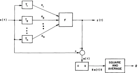
(a) We shall define a set of functionals {Ti} by which the random variables {ai} are derived from x(t), that is, ai = Ti[x(t)].

(b) For transforming the set {ai} into a function z(t) which in some sense approxi-mates x(t), we need to define an approximation function F for which z(t) = F(t, al, ... , an).

(c) We must state in what sense z(t) approximates x(t) by introducing a norm on the error, e(t)[| = x(t)-z(t)t)11. (In general, it would not be necessary to restrict ourselves to a norm here; however, it is convenient for our purposes.) This norm shall comprise the criteria for the relative importance of the characteristics of x(t).

(d) We must utilize a statistical property of

j|

e(t)|| to obtain a fidelity measure across the ensemble of x(t). In this report we use = E[II e(t)II 2], although others could be defined. (For example, P[ e(t)| k]. It may be well to point out, however, that the choice of the expected value is not arbitrary but made from the standpoint of analyt-ical expediency.) We shall sometimes refer to as "the error."

x( t)

8

Fig. 2. The process of fidelity measurement of a discrete representation.

14

The process of fidelity measurement of a discrete representation would then be as shown by the block diagram in Fig. 2.

We are now in a position to state the fundamental problem in the study of the discrete representation of random signals. We must so determine the set {Ti} and F that

= E[ IIx(t)-F(t, al, ... an) 12] (11)

shall be a minimum. We shall denote this minimum value by * and the Ti} and F for which it is attained by {T*} and F*. In many cases the requirements of the problem may force the restriction of {Ti) and F to certain classes, in which case we would per-form the minimization discussed above with the proper constraints.

It is certain that the solution of this problem, in general, would be a formidable task. We shall be dealing largely with those cases in which {Ti) and F are linear and the norm is the square root of a quadratic expression. This is convenient because the minimiza-tion of Eq. (11) then simply requires the soluminimiza-tion of linear equaminimiza-tions.

3.2 LINEAR REPRESENTATIONS IN A FINITE TIME INTERVAL

We shall now consider a random process x(t) to be represented in a finite interval of time. We shall assume that (a) the approximation function F is constrained to be of no higher than first degree in the variables a, ... , an, and (b) the norm is f(t) I =

~[&xf(t)

dt

j

, where the interval of integration, Q2, is the region of t over which the process is to be represented.

Considering t as a parameter, we see that F(t, al,..., an) may be written n

F(t,a₁ ... an) = c(t) + ai4i(t)

i=l

We then want to minimize

= E x(t) - c(t) -i= aii(t) dt (12)

The minimization will be performed, first, with respect to the functionals {Ti} while F is assumed to be arbitrary (subject to the constraint) but fixed. There is no restric-tion in assuming that the set of funcrestric-tions {+i(t)} is an orthonormal set over the interval 2, for if it is not, we can put F into such a form by performing a Gram-Schmidt orthogon-alization.4 8

We have then f i( t) j(t) dt = 6ij, where ij is the Kronecker delta.

It follows from the minimal property of Fourier coefficients that the quantity in brackets in Eq. (12) is minimized for each x(t) by the choice

15

ai = Ti[x(t)] = [x(t)-c(t)] i(t) dtn

over all possible sets {Ti}. Likewise, it follows that its expected value, 0, must be minimized. Setting y(t) = x(t) - c(t), we see that the minimized expression is

S=

E

Y(t)

- i(t) y(s) (i(s) ds dt

i=l n

= Ry(t,t) dt-

j

5'

R(s,t) i(s) i(t)dsdt By the corollary of Theorem I, we know that

n

1i=

1

n n

R y(s,t) i(s) i(t) ds dt

7

C 2Ry(st) i(s) yi(t) ds dt= ki

i= 1 i= 1

where the Xi and the yi(t) are the eigenvalues and eigenfunctions of the kernel Ry(s, t).

O is then minimized with respect to the 4i(t) by the choice 4i(t) = Yi(t). The error now is

e = Ry(tt) dt - . 1 i=

From Mercer's Theorem (see section 2.2), we have oo0

Ry(s,t) = \ kiyi(S) Yi(t) i=l so that Ry(t, t) dt and therefore oo i=l

We now assert that each have for each eigenvalue

eigenvalue is minimized by choosing c(t) = mx(t) = E[x(t)]. We

16 co =

I

i i=l n -X ki i=l oo i=n+l X. 1

I

i= l, ... ,n

Ry(s,t) i(s) i(t) ds dt

E[x(s)x(t)-x(s)c(t)-c(s)x(t)+c(s)c(t)] i(s) Yi(t) ds dt

Rx(, t) y(s) Y i(t) ds dt - 2 r(s) yi(t) ds c(t) yi(t) dt

2

c(s) i(s) ds] Now, since

c(s) yi(s) ds -

S

_mx(

_s)

Y.(s) ds d 2i() > 0

We have

IS

(

S1yifs)

dS2

c(s) yi(s) ds

- 2 mx(s) yi(s) ds

SQ

-s,2

mx(s) yi(s)

Here, the equality sign holds for

2 mx(S) yi(s) ds = c(t) yi(t) dt

After applying this inequality to Eq. (13) we find that Xi is minimum for

n

mx(s) i(s) ds =

S

c( t) dt

and since we want this to hold for all i, we have c(t) = m(t).

So, we finally see that if we have a random process x(t) with mean mx(t) and covar-iance function rX(S, t) = E[{x(s)-mx(s)}x(t)-mx(t)}], then is minimized for

n

F (t,al I... an) = mx(t) + i= 1

aiYi(t)

The yi(t) are the solutions of

rx(s, t) yi(t) dt = kiyi(s) sE 2

arranged in the order 1 2 ... , and

17

xi=

=S

SQ

2

=S,

2

S

2

(13)

2

--- --- 1 1_ _ _ I I_ ^- I _ c(t) i(t) dt

*

a.

S

x(t) yi(t) dt - m(t) y(t) dt The minimum error is, then,

n 00

0*= r(t,t) dt- iX.= (14)

i= 1 i=n+1

This solution is identical to the Karhunen-Loeve expansion of a process in an ortho-normal series with uncorrelated coefficients which was described in section 2.4. This was first proved by Koschmann,21 and has since been discussed by several other authors 1 3, 5, 22

We have assumed that x(t) has a nonzero mean. In the solution, however, the mean is subtracted from the process and for the reconstruction it is added in again. In the rest of this report we shall consider, for the most part, zero-mean processes, for if they are not, we can subtract the mean.

3.3 A GEOMETRICAL DESCRIPTION

A useful geometric picture can be obtained by considering a random process in a finite time interval as a random vector in an infinite dimensional vector space. This geometric picture will be used in this section in order to gain understanding of the result of section 3. 2, but we shall confine ourselves to a finite m-dimensional vector space. The process x(t) will then be representable as a finite linear combination of some ortho-normal set of basis functions {Ji(t)}; that is,

m

x(t)= E xii(t) i= 1

where the xi are the random coordinates of x(t). We see, then, that x(t) is equivalent to the random vector x= {Xl, ... ,Xm}.

We shall assume that x(t) has mean zero and correlation function Rx(s, t). The ran-dom vector x then has mean zero and covariance matrix of elements rij = E[xixj], with

m m

R(s, t) = E riji(s) ,j(t) i=1 j=l

Our object is to represent x by a set of n random variables {al, . . ., an}, with n < m. Using arguments similar to those of section 3. 2, we see that we want to find the

n 2

random vector z = c + ai i which minimizes 0 = E[ix-zI2]. Since x has zero mean,

i= 1

we shall assume that c = 0. Then, z is a random vector confined to an n-dimensional hyperplane through the origin. Since the set {i} determines the orientation of this plane, there is no restriction in assuming that it is orthonormal; that is, = ij. If we

x 3

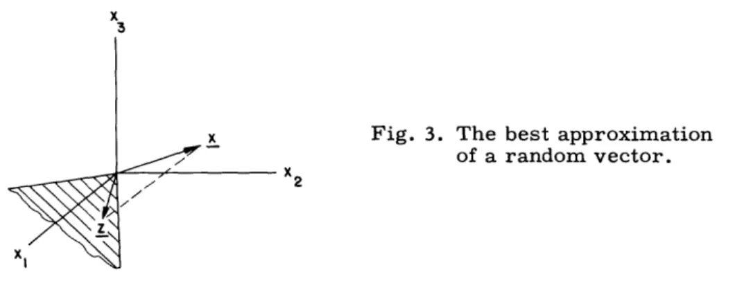
Fig. 3. The best approximation of a random vector. X2

are given a particular orientation for the plane, that is, a particular set {4i}, and a par-ticular outcome of x, then it is clear that the best z is the projection of x onto the plane,

n

as shown in Fig. 3. That is, z= (x,i> , i, so that ai = (x,i>, (i=l,...,n). This is related to the minimal property of Fourier coefficients, as mentioned in section 3. 2. The error, 0, then becomes

0=E[Ix-zl

I

n n

i=1 i=l1

=E[lxI ]-E[ (x,4i)] ₍₁₅₎

Now, we must find the orientation of the hyperplane which minimizes 0. From Eq. (15), we see that this is equivalent to finding the orientation that maximizes the average of the squared length of the projection of x. We have for the inner product

m OE +i= xij

j=l

where i = {il'' *im}' Then

Z 0 = E[lxl - E xjqi} n m m = E[Jx 2 ] -i 1 k- ij-i=1 j=l k=1 19

_____ _I

I _

II_

The quantity in brackets is a quadratic form m

-[ail,.. I

*im]- E

j=1 so that we must maximize

n

i=l

where {i} is constrained to Suppose that n = 1, than I 1 1 = 1. By the maximum that

be an orthonormal set.

we must maximize f[ 1 1l . .. im] subject to the condition

property of the eigenvalues mentioned in section 2.2 we see

max ,[al] = -[y] = 1

11I = 1

where 1 is the largest eigenvalue of the positive definite matrix [rij], and y1 is the

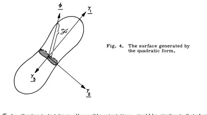
corresponding eigenvector. So we have the solution for n = 1. The surface generated

_> ;

Fig. 4. The surface generated by the quadratic form.

r4t

by -F, by allowing

l1

to take on all possible orientations, would be similar to that shown m

in Fig. 4 for m = 3. This surface has the property that Z

[i]

is invariant with

m i=

-respect to the set {a} and is equal to Z i.. This must be so, since if all m dimensions i=l 1 20 m k=l rjkAij ik

Is

I

are used in the approximation, the error must be zero.

By the maximum property of the eigenvalues, we also have max 9-[+i] = [-Yi] = i

i -

-Ki,

Yj) =

1

j = 1,...,i-1

So, from this property and by observing Fig. 4 we might expect that n max I = {4i}i= I n n E H--i]= xi i=1 i=1

This is in fact true, but it does not follow so simply because in this procedure the max-imization at each stage depends on the previous stages. The fact that it is true depends on the character of the surface, and it follows from Fan's Theorem (section 2.4). 3.4 MAXIMUM SEPARATION PROPERTY

There is another geometric property associated with the solution to the problem of section 3.2. Let r be an m-dimensional linear vector space the elements of which are functions over a certain time interval Q. Suppose that the random process x(t) consists only of certain waveforms sl(t), . . sn(t) which occur with probabilities P1, . ., Pn

Only one waveform occurs per trial. The autocorrelation function is, then, R x(s, t) = n

Z Pisi(s) si(t), and we shall assume that E[x(t)] = 0. i=l

Suppose that we arbitrarily pick a set of orthonormal functions y1(t), ... , yq(t)

which define an 2-dimensional hyperplane r of r. Let y,+l(t) , ,m(t) be an arbi-trary completion of the set so that {yi(t)} is a basis for the whole space. The projections of the waveforms on rI are, then,

2 2

s (t) = yj(t) s(t) yj(t) dt = IYj(t)

j=1 j1

i= 1,...,n

where

j = ·.. · m We shall define the average separation S

n S ij= i, j= of the s(t) in r₁ I to be

P j , [si(t)-s(t)]

2

dt

21 --

_1^_1_1

1_

_ --- _ I sij s it) yj ( dt

and we shall be interested in finding what orientation of r maximizes S. k=l We have PiPj (Sik-Sjk) PiPj S2k + n i, j= 1 k=l {n I ki= I PiPjSjk - Z2 jk n i, j1 I Pijsikij k=l PiSik} -2 k=l We note that n E[x(t)] = i= 1 PiSi(t) =_11i m = Yj(t) j= 1 n i=l n n

i Pi

i=1 j=1 P.s.. = 0 1 1J therefore n i=l P.s.. = 0 1 1J n S=2

Z

i= 1 n = i=1 k=l j = ,...,m PiS2 i ik PiSS

SA

R (s, t) =2 1 k=l

As we have seen before, this is maximized by using the first eigenfunctions of Rx(s, t) for the yl(t), .. ., yq(t), so that the orientation of r which maximizes the average sep-aration is determined by these.

22 n i, j 1 n =2 i=l k=l k=l PiS2 i ik Sij YjIt) and n S Si(S) Silt) yk (S) k(t) ds dt 'Yk(s) yk(t) ds dt

Consequently, we see that if we have a cluster of signals in function space, the orientation of the hyperplane which minimizes the error of representation in the lower dimension also maximizes the spread of the projection of this cluster on the hyperplane, weighted by the probabilities of occurrence of the signals. If there were some uncer-tainty as to the position of the signal points in the function space, then we might say that this orientation is the orientation of least confusion among the projections of the signal points on the hyperplane.

3.5 THE ASYMPTOTIC BEHAVIOR OF THE AVERAGE ERROR IN THE STATIONARY CASE

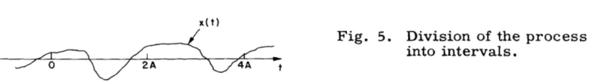
In this section we shall consider the representation of a stationary process x(t) for all time (see Jordan1 6). This will be done by dividing time into intervals of length ZA and using the optimum representation of section 3.2 for each interval. Since the process is stationary, the solution will be the same for each interval.

x(t)

Fig. 5. Division of the process

into intervals.

/ 2A \ 4A t

Suppose that we use n terms to represent each interval. We then define the density as k = n/ZA, or the average number of terms per unit time. If we consider an interval of length 4A, as shown in Fig. 5, consisting of two subintervals of length 2A each sepa-rately represented, we would have an average error

20*(ZA) 0 (ZA)

4A - ZA

If we now increase the interval of representation to 4A while using Zn terms, that is, 0*(4A)

holding the density constant, we would have an average error 4A . It is certainly true that

0*(4A) 0*(ZA)

4A 2A (16)

since if it were not true, this would contradict the fact that the representation is opti-*(ZA)

mum. It is the object of this section to study the behavior of ZA as A increases while the density is held constant.

Since the process is stationary, Rx(t,t) = Rx(0), and, from (14), we have n

1 0*(ZA) = Rx(0) 2A i

i=l

23

-where the Xi are the eigenvalues of 1

Rx(s-t) 4i(t) dt = Xkii(s) -A s A

Since n = 2kA must be a positive integer, A can only take on the values n

A _{n 2k}-- n= 1,2,...

The sequence

0*(ZAn )

ZA is monotonically decreasing because of the argument leading to n

(16). Since 0*(2A ) 0, all n, the sequence must have a limit.u ~ We want to find

0*(2A ) im Z2A = R (0) n-oo n 2kA n - lim 2A n o0 n ,

We now make use of a theorem that will be proved in Appendix B. THEOREM II. 2kA_n lim 2A E i= n · = lim k n n n-oo i=l X. = I SE Sx(f) df where

S(f)

= oo Rx(t) e-j2 f t dt

and is the power density spectrum of the process, and E = [f; Sx(f) ]

where is adjusted in such a way that

[E] = k

(The notation [f; Sx(f)a>] means "the

measure of the set E, or length for

set of all f such that Sx(f) ¢A." our purposes.) Now since

A[E] denotes the

RP( ) =

S0o

00 RX(t) = o Rx(0) = ~7oo Sx (f) ej ft df Sx(f) df and 24 A -A (17)

0*(ZA) 00

lim 2A Sx (f₎ df - Sx (f) df S= S(f) df (18)

n- oo n 00

where E' = [f; Sx(f)< 2].

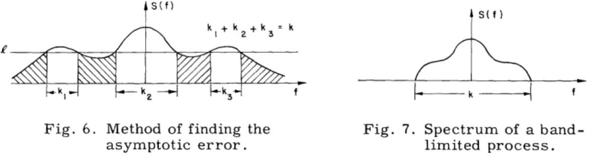
In other words, we take the power density spectrum (see Fig. 6) and adjust in such a way that the length along f for which Sx(f) > 2 is k and then integrate over all the remaining regions. This gives a lower bound for the average error and the bound is approached asymptotically as A increases.

iS(f)

kl+ k2+k 3 k

klW k 2k f |^ k - | f

Fig. 6. Method of finding the Fig. 7. Spectrum of a band-asymptotic error. limited process.

If the process x(t) is bandlimited with bandwidth k/2 cps, that is, it has no power in the frequencies above k/2 cps, then we have the spectrum shown in Fig. 7. If we then use a density of k terms/sec, we see that must be adjusted, according to the condi-tion of Eq. 16, to a level = 0. By Eq. 17, we have

lim 2A x(f) df= 0

n-oo n E'

This implies that we can approach arbitrarily closely an average error of zero with a finite time linear representation by allowing the time interval to become large enough. This is in agreement with the Sampling Theorem 2 8' 1which states that x(t) can be repre-sented exactly by R equally spaced samples per unit time; and, in addition, we are assured that this is the most efficient linear representation.

3.6 A RELATED CASE

Suppose that x(t) is a zero-mean random process in the interval [-A, A] with auto-correlation function R x(s, t). We now consider the problem in which the ai are specified to be certain linear operations on x(t)

A

ai= A x(t) g(t) dt i= 1 .. ,n

and we minimize with F constrained as in section 3. 2; that is, n

F(t,al, .an) = ) ai4i(t) i=l

(c(t) = 0, since the process is zero mean). If we follow a straightforward minimization procedure, we find that the set {qi(t)} must satisfy

Rx (t, s)gi(s) ds = j(t) Rx(u, v) gi(u) g(v) du dv j=1l

i= 1,...,n

which is just a set of linear equations in a parameter t.

If the ai are samples of x(t), we then have gi(t) = 6(t-ti) and the set {i(t)} is then the solution of

j(t) Rx(ti, tj) i= 1,...,n (19)

Solving this with matrix notation used, we have

qj(t)] [Rx(ti, tj)]- 1 Rx(t, t)]

If we consider (t)] for t = ti (i=, .. . ,n), then we have the matrix equation

[wj(ti)] = [Rx(ti,t)]-l [Rx(t i, tj)] = [I]

where [I] denotes the identity matrix, so we see that

4j(t)

= {1:

0 O t = t. J t = t₁i, j = 1,...,n i #j

If the process x(t) is stationary and the ai are equally spaced samples in the interval

(-oo,oo), Eq. (19) becomes

R (t-kT ) = _{Oj(t) Rx(kTo-2To)} k = 0, 1, -1, 2, -2. . .

2=-oo

where T is the period of sampling. oo

Rx(t') = E p(t'+kTo) Rx(kTo

= -oo

Substituting t' = t - kTo, we get

-iT.) k = 0, 1, -1, 2,-2...

This holds for k equal to any integer, so that

26 n

R (t, ti ) =

00 Rx(t') =

2=-00

00 - - 0o 2=-oo 4)2(t'+(k+j)To) Rx((k+j)To-fTo) 10+j(t'+(k+j)To) Rx(kTo-T) o and we have $1(t+kTo) = +j(t+(k+j)To) or $1+j(t+kTo) = $2(t+(k-j)To) so that for = 0, k = 0 4j(t) = o0(t-jTo) where j = 0, 1, -1, 2, -2, ....

interpolatory function, which is the solution of oo

Rx(t) = =-0oo

The set {4j(t)} is just a set of translations of a basic

4o(t'+fTo) Rx(2To)

This problem has been studied by Tufts.3 0 case is

He has shown that the average error in this

R n - C0 - % 1_x-e

[Sx(f)]

oo z Sx(f-2fo) = - oo00 df (20) where f= 1/T. 3.7 AN EXAMPLE

Let x(t) be a stationary random process in the interval [-A, A] with a zero mean and autocorrelation function

Rx(s,t) = Rx(s-t) = r e-2ris-t

The power density spectrum is then S x(f) = I

1 + f

The eigenfunctions for this example are

27 II. II . 4

i, odd i, even Ci cos bit %i(t) = cisin b.t 1

where the ci are normalizing constants and the bi are the solutions of the transcendental equations b. tan b.A = 2r 1 1 b. cot bA = -2w 1 1 i, odd i, even

The eigenvalues are given by 4wr2

%.

1 b.2 2 + 4 22

The details of the solution of this problem have been omitted because they may be found elsewhere. 5 2

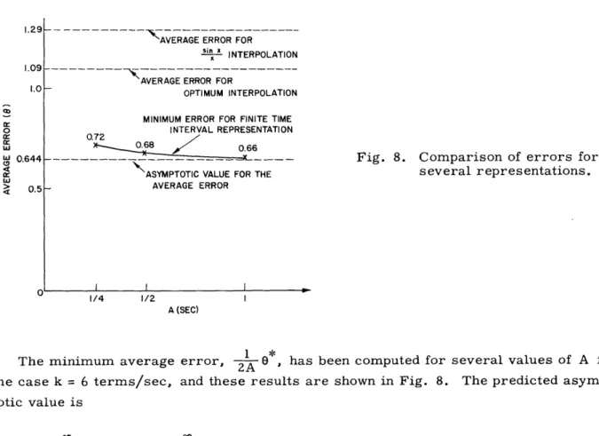
"AVERAGE ERROR FOR

sin x

x INTERPOLATION

OPTIMUM INTERPOLATION

MINIMUM ERROR FOR FINITE TIME INTERVAL REPRESENTATION 0.72

_____Z 0.66 "ASYMPTOTIC VALUE FOR THE

AVERAGE ERROR

Fig. 8. Comparison of errors for several representations.

I I

1/4 1/2 I

A (SEC)

The minimum average error,1 , has been computed for several values of A for the case k = 6 terms/sec, and these results are shown in Fig. 8. The predicted asymp-totic value is k/2 Sx(f) df 2 1 2 df = . 644 28 (21) 1.29 1.09 1.0 0u n-'r w J 0.644 0.5 < 0.5 -__- -- - -N7 , -.I

~

clen c~ _

I-This is plotted in Fig. 8 along with the error incurred by sampling at the rate of 6 samples/sec and reconstructing with sin _x interpolatory functions. This error is just twice the error given in Eq. 31, or twice the area under the tails of the spectrum for If > 3. This is a known fact; but a short proof will be given in Appendix C for reference. Also shown in Fig. 8 is the error acquired by sampling and using an opti-mum interpolatory function. This error was computed from Eq. (20).

3.8 OPTIMIZATION WITH UNCERTAINTY IN THE REPRESENTATION

It is of interest to know whether or not the solution of section 3.2 is still optimum when the representation in the form of the set of random variables {ai} is subject to uncertainties. This would occur, for example, if the representation is transmitted over a noisy channel in some communication system.

In the following discussion we shall assume that the process is zero-mean; the representation is derived by the linear operations

ai = x(t) gi(t) dt, (22)

and the approximation function is n

F(tal,..,an) =

7

aii(t). i=l 1

Our object is, then, to determine under what conditions

n 2

= E[ [x(t) (ai+Ei(t)] dt] i=l

is minimized, when the Ei are random variables representing the uncertainties. Under

the assumption that {di(t)} is an orthonormal set, we obtain

O = R(t, t) dt - ZE (a+E (t) (t) dt + E(ai+Ei)2

and we substitute Eq. 22 to obtain

n n O=

5

x t - E Rx(s, t) g(s) .i(t) ds dt +

SRx(s

t) g₁(s) gi(t) ds dt i=l i=l n n n

S

E[ i x( )] i (t)) ix(t)]+ d E[i2]. (23) i= 1 1 i= 1 i= 29 _________II

If we replace gi by gi + ali in this expression, we know from the calculus of variations5 3 that a necessary condition that 0 be a minimum with respect to gi is

a a=0

Applying this value, we obtain

aa |O =2 =

S

'i ) ( s, t) (t) dt - i(t) Rx(s, t) dt - E[Eix(s)]} = 0 and since i(s) is arbitrary, the condition becomes

S

Rx(s, t)[)i(t)-gi(t)] dt = E[Eix(s)] sE i= l, ... ,n

It is seen, then, that if E[Eix(s)] = 0, s E 2, then +i(t) = gi(t) (i=l, ..., n) satisfies the

condition. (If Rx(s,t) is positive definite, this solution is unique.) For this case, Eq. (23) becomes

n n

0

=

(t, t) dt

-

'5

R(s, t) ci(s) i(t)

ds dt

+

C

E[E

2

j

i= 1 i=l

Consequently, we see that if E[Eix(s)] = 0 (i=l,.. ., n), for all s E 2, then the solution of section 3.2 is still optimum and the minimum error now is

n n

0* = R(t,t) dt - + i E[ E]. i=l i=1

3.9 A MORE GENERAL NORM

Although in the general formulation of the problem given in section 3. 1 we consider a general norm, up to this point we have made use of only the rms norm. In many prob-lems, however, we shall be interested in a measure not only of the average difference between functions but also of other characteristics of the functions. For example, in Section I we described in what way a linear representation of the past of a random proc-ess is useful in a characterization of nonlinear systems. For the most part, such a

characterization is useful only for those nonlinear systems for which the influence of the remote past on the operation of the system is small compared with the influence of the immediate past. In such a case, we would be interested not in a norm that weights the average difference between functions uniformly over function space, as in the rms norm, but in a norm that weights the immediate past more heavily than the remote past.

In this problem we might also be interested in a norm that discriminates not only in time but also in frequency. The high frequencies may influence the operation of the system to a lesser degree than the low frequencies. So, we see that it would be of inter-est to consider a norm that is more general than the rms norm which discriminates neither in time nor in frequency.

We consider here a generalization on the rms norm which allows more general dis-crimination in the characteristics of the random function. This norm has the additional property that with it the solution of the representation problem still requires only the solution of linear equations. This norm is

1/2

I|f(t)I

=

SfIt

dt]

Here, fl(t) is obtained by operating linearly on f(t); that is,

fl(t) =

5

K(t, u) f(u) du; t E Q (24)

where K(t, u) is determined by the requirements of the problem. (We have assumed that the linear operation is an integral operation, although this is not necessary. In our first special case below it will not be strictly an integral operation.) Essentially, what we have done is to pass the error e(t) through a linear filter and then use the root mean square. In order for this to be a true norm, K(t, u) must satisfy the condition

S

K(t, u) f(u) du = t E 0 (25)

if and only if f(u) = 0 for u E Q2. (See sec. 2. 1.) A necessary and sufficient condition that this be true is that the symmetrical kernel

Kl(s, t) = K(u, s) K(u, t) du

be positive definite. This is because the conditions

fl(t) = i K(t, u) f(u) du = 0

an t dt = K(tu) K(tv) dt} f(u) f(v) du dv =

are equivalent.

The error, , now becomes

31

-=

ES

dt K(t, u) (u) - c(u) aii i(u) du

n 2

= Ei dt K(t, u) x(u) du - K(t, u) c(u) du -

7

a.

i

K(t, u) iu) du

so we see from the second of these equations that the problem reduces to the representa-tion of the process

y(t) = K(t, u) x(u) du

by the method of section 3.2.

F *(t, al, ... ,an) = mx(t)

Consequently, our solution is n

+

7

ai'i(t) i= 1

in which the yi(t) are solutions of

(i(t) = K(t, u) yi(u) du

and the (Di(t) are the eigenfunctions of

G(s, t) i(t) dt = ii(s) arranged in the order 1 > 2 > ....

G(s, t) = G(s, t) is found from K(s, u) K(t, v) r(u, v) du dv and we have ai i a. ds~(s) K(s, v)[x(v)-mx(v)] dv. The minimum error is

S

=

G(t, t) dt G (t, t) dt -n i=1l (30) i 32 (26) (27) (28) (29) G (s, t) ( i(s) (D(t) d dt X. =1j

in which the Xi are the eigenvalues of Eq. (28).

We have a particularly simple case when K(s, t) is expressed over the basis of eigen-functions {i(s)} of rx(s, t); that is,

00

K(st = ) Piti(s) i(.)

i= 1 We then have for G(s, t)

G(s, t) =

i=1

iai1i(s) i( t)

where the ai are the eigenvalues of rx(S, t).

1x We then have i(s) = i(s) ki₁ = ₁₁ai 1 vi(s) = 1i si( ) for i = 1, 2, ....

We shall now discuss two special cases of this norm which demand special attention. THE FIRST CASE

First, we consider the rms norm weighted in time, that is, we have

I1

f(t)

j

=

5

W2(t) f2(t) dt

so that the linear operation is just multiplication by W(t). K(t, u) = W(t) 6(t-u).

This corresponds to a kernel

The solution now is n mi(t) F (t, al ... an) = m(t) + ai W(t) i= 1

SQ

W(s) r(S, t) W(t) i(t) dt = Xi iX 1 1 (S) ai S W(t) i(t)[x(t)-mx(t) ] dt

in which the error is

33 1/2

c

s £E

n *W 2 t) (t t) dt W(s r(s, W(s) t) W(t) cD(s) .(Dt) ds(t, dt i=l n = i W2(t) r(tt) dt -

Z

Xi i=l

This is of special interest in the nonlinear filter problem in which we want to repre-sent the past of a random function with a norm that minimizes the effect of the remote past. In fact, if the process is stationary, we must use this weighted norm in order to get an answer to the problem at all. This is because if we use the method of section 3. 2, the first term of Eq. (14) would be infinite; that is,

S0

r(O) dt = oo

and no matter how many terms we use, we would not improve the situation. Also, the kernel of the integral equation

0

_ rx(s-t) yi(t) dt = kiyi(s) S [0, O]

is not of integrable square; that is, we have

SS_

rx(-t) 12 dsdt = oo

so that we are not assured that the integral equation has a countable set of solutions. However, if we use a weighting function W(t) chosen in such a way that

i W4 (t) rx(O) dt = rx(O) W (t) dt

is finite, then we can find a solution.

It might be well to point out also that although we have said that we must pick a weighting W(t), we have not attempted to suggest what W(t) to use. This must depend upon the nonlinear filtering problem at hand and upon the insight and judgment of the designer.

As an example we consider the zero-mean random process x(t) with autocorrelation function Rx(s, t) = e s - t [ We shall be interested in representing the past of this pro-cess with a weighting function W(t) = e over [--o, 0]. However, for the sake of

conven--t

ience, we shall use the interval [O, co] and weighting function W(t) = e . In this case the solutions of the integral equation17

34

00 s 0 are 1i(t ) = Ai et J e 2

i-

2 qi (31)

Here, the qi are the positive roots of Jo(qi) = 0. The Ji(x) are the Bessel functions of

the first order, and the Ai are normalizing constants. The error in this case is

8* =

*$

n n

e -Z dt -

xi= -Z

xi

i= 1 i= 1

The first two zeros of Jo(x) are5

ql = 2.4048 q2 = 5.5201

so that the first two eigenvalues are

k1 = 0. 3458 k2 = 0. 0656

The error for one term is then

8 = 0.5 - 0. 3458 = 0. 1542 (32)

and for two terms

82 = 0.5 - 0. 3458 - 0. 0656 = 0. 0886 (33)

THE SECOND CASE

Second, consider the case in which the interval of interest is [-oo, oo], and the kernel of the linear operation of Eq. (24) factors into the form

K(s,u) = Kl(s) K2(s-u)

so that we have

fl(s) = Kl(S)

S

K2(S-U) f(u) du

35

__1_11

e-s

e- S-t e-t

~

t t=XI S

Thus, the operation consists of a cascade of stationary linear filtering and multi-plication. If Kl (s) >- 0 and the Fourier transform of K2(s) is real and positive, then

we can consider the norm as a frequency weighting followed by a time weighting. (For these conditions, the condition of Eq. (25) for the kernel of the norm is also satisfied.) Let us consider the example of the representation of white noise x(t) of autocorrela-tion funcautocorrela-tion Rx(s, t) = 6(s-t) and mean zero. Here we use as weightings

2 -s Kl(s) = e 2 -s K2(s) = e

that is, Gaussian weightings both in time and frequency. that we must find the eigenfunctions of G(s, t), where

G(s,t) =

55

= S700

From Eqs. (28) and (29) we see

K1(s) K2(s-u) K1(t) K2(t-v) Rx(u, v) du dv s2 2 _ 2 t 2 e e et e(t- v) (u-v) du dv -s2 t2 =e e -t 2 The Fourier transform of e

-t 2 -j2ft e e dt=we -(s-u)2 e-(t-u) du (see Appendix D) is -r2f2 lT f we know that f(o') g(t--) do- = -oo -oo F(f) G(f) ej2wft df

where F(f) and G(f) are the Fourier transforms of f(t) and g(t). We then have

00

rX

U-o -u 2 -(s-t-u) du2 r e e du = Tr e-2r 2 f 2 _{ej2rf(s-t) dt} e e d ; - I (s-t) = 2 e so that (s, t) 2 t2 - 1 (s-t)2 G(st) = T - se e e 36 -oo

Q

It is shown in Appendix D that the eigenfunctions of this kernel are

At2 d i -2 2t 2 (D (t) = Ai e - e

i 1 1

~dt

dt11

i = 0, 1,. . .

Here, the Ai are normalizing constants and the eigenvalues are

X. = / 1 (32-f)i 1 \/ 3 + 2

i = 0 1, ... .

It is seen that these functions are the Hermite functions modified by a scale factor. Hermite functions5 5 are given by

Hn(t) = (2nn! -)-1/2 et2/2 dn dtn -t 2 e n= 0, 1,2, ... Therefore, we have i (t) = (Z2)1/4 Hi[(2-Z)1/Z t] and the Ai are given by

A = (2X) /

(Zi! 1/

i = 0, 1, 2,...

i = 0, 1, 2, ...

Referring to Eq. (26) we see that in order to have the complete solution we must find the Yi(t) that are the solutions of

1 (t) = _cooc X0 -t e (t-u) 2 e e ¥ i(u) du i = 0, 1, 2, ... according to Eq. (27). It is yi( t ) = Ai (- e)

shown in Appendix E that the solution is

l+NJTz t2 2 + NJZ? di e dt

- Tit

2

so that the best representation is given by

F (t, a, .. . an) = i=O 1+Nf 2 t (JT+2)1 2 + J a.A. e 1T V( 2 -,47) ds A. e (NZ-l)s2 d e-Z2Zs2 1 ds1 di _-J t2 e dt1 e- ( s - t ) x(t) dt 37 The and a₁ co

___

i·_

._ _

-and the error is 0 = n 2 0 i=O n e dt -i=O 3 (3_22-i

3

+ 2z,

2

2_ / 4 (3_-2J-)i 23 + ZJ

3.10 COMPARISON WITH LAGUERRE FUNCTIONS

We now return to the first example of section 3. 9, but this time we use Laguerre functions in place of the functions of Eq. (31). We shall be interested in just how close we can come to the minimum possible error given by Eqs. (32) and (33). The Laguerre functions 5 6 are given by

L (x) = - e n (xe )

n+l _{n dx}n n = 0, 1, 2, ...

for x 0.

Since orthogonality of functions over [0, oo] is invariant with respect to a change in scale, we have a degree of freedom at our disposal. The Laguerre functions given above satisfy the relation

00

0 Li(y) Lj(y) dy =

1 i=j

0 i j

and if we make the change of variable y = ax, we have

a Li(ax) L.(ax) dx =

0 J~~~~

{

1 i=j

0 i*j

from which it follows that the set of functions F Ln(ax) is orthonormal. We shall be interested in picking a best scale factor a for a representation in terms of these functions.

By replacing the functions Di(t) in Eq. (30) by the set NJa Ln(ax), we obtain for the error

n

0 = W() x(t, t) dt - E

sO

i=1

and for the example it becomes

38

(34)

n

=

-2 1

i= 1

e-s-t e- s-t aLi(as) Li(at) ds dt.

Suppose that n = 1. The first scaled Laguerre function is

a

TJaL (ax) = IN e G 1

so that we have for the error

1 2r° e-s-t -I s-t

as at 2 2

a e ds dt

which on performing the integration becomes

(a)- (a+ )(a+4) 1 2 (a+Z)(a+4)

This error is shown in Fig. 9 plotted as a function of a. for which 01(21sT) = 0. 157. 0.5 0.4 0.3 0.2 0.1 It has a minimum at a = Zq2'

I

Fig. 9. . 8 (a) 92(a) I I I I I I

The error as a function of scale factor for Laguerre functions.

I 2 3 4 5 6

Now suppose that n = 2. The second scaled Laguerre function is

NFa L₂(ax) = -(e ax/2 ax eax/2 and the error becomes

(a)

=2 (a+2)(a+4) Oz- Z (a+Z)(a+4)

e-s-t-I s-tl ae -as/ -as/Z][e-at/Zat e- at/2] ds dt

39

-

S

00

___1___1111_1111^____I -- ----i

which on performing the integration becomes

1 4

a 4a(a 3-4a-1 6)

2(a)- 2 (a+2)(a+4) (a+2)3(a+4)2

1 -a5 + 16a3 - 32a + 128

2 4 3

(a+2) (a+4)

This is also shown in Fig. 9 and it is minimum at a = 4, for which 62(4) = 0. 093. We see, first of all, that the best scale factor for n = 1 is not the same as it is for n = 2. Also, it is interesting that the performance of the Laguerre functions for the best scale factor is remarkably close to optimum. The minima of the curves in Fig. 9 are very nearly the values given in Eqs. (32) and (33).

This example illustrates the value of knowing the optimum solution. In practice, if we are interested in representing the past of x(t), we would derive the random variables ai from x(t) by means of linear filters. In this example, the synthesis of the

filters for the optimum solution would be much more difficult than the synthesis of the filters for Laguerre functions. For representing the past of x(t) we would have (reversing the sign of t since in the example we have used the interval [O, oo])

0

x(t) et

Ai

e

1/+

et] dt

so that we would use a linear filter of impulse response

hi(t) = Ai e J1I - t

1 1 1

which would not be easy to synthesize. Now, if we use Laguerre functions we would have

0

ai = x(t) et J Li(-at) dt

and we would use a filter of impulse response

hi(t) = e- t Li(at) (35)

which is quite easy to synthesize and gives us an error very close to optimum. By means of cascades of simple linear networks we can synthesize impulse responses in the form of Laguerre functions 2 3 or other orthonormal sets of the exponential type. ll In Eq. (35) we have a multiplying factor of e- t which can be accounted for in the complex

40