Distributed physical simulations and synchronization in virtual environments

Distributed Physical Simulations and Synchronization in

Virtual Environments

by

Martin Richard Friedmann

THE UNIVERSITY OF MICHIGAN, ANN ARBOR, 1988 SUBMITTED TO THE MEDIA ARTS AND SCIENCES

SECTION, SCHOOL OF ARCHITECTURE AND PLANNING IN PARTIAL FULFILLMENT OF THE REQUIREMENTS FOR THE DEGREE OF

Master of Science

MASSACHUSETTS INSTITUTE OF TECHNOLOGY Feburary 1993

@

Author ... .. ...

Certified by ... ...

Accepted by ...

Media Arts and Sciences Section October 31, 1992

Alex P. Pentland Associate Professor Computer Information and Design Technology Thesis Supervisor

Stephen Benton Chairperson Departmental Committee on Graduate Students MASSACHUSETTS INSTITUT

OF TECHNOLOGY

MAR 11 1993

LIBRARIES

Distributed Physical Simulations and Synchronization in Virtual

Environments

by

Martin Richard Friedmann

Submitted to the Media Arts and Sciences Section, School of Architecture and Planning on October 31, 1992, in partial fulfillment of the

requirements for the degree of Master of Science

Abstract

This thesis addresses problems fundamental to the creation of interactive 3D graphics appli-cations which feature real-time simulations carried out on distributed networks of computer workstations. Sufficient lag exists in present day hardware configurations to stifle realism, even when the computer simply mimics the sensed actions of users with rendered graphics. This problem is compounded when real-time physical simulations and more remote users are added. Even if the simulation algorithm is efficient enough to provide a timely and realistic reaction to inputs, the system must still further overcome subsecond lags in the sensor and rendering pipelines, to achieve spatio-temporal realism.

First, a framework for distributing the real-time execution of non-rigid physical simulations is presented. This framework has been demonstrated to have an efficiency that increases nearly linearly as a function of the number of processors. To achieve this scaling behavior one must minimize network and processor contention; in our system this is made possible by replacing synchronous operation by the weaker condition of bounded asynchrony, and by use of compact modal representations of shape and deformation. The system also allocates computational resources among networked workstations using a simple, efficient "market-based" strategy,

avoiding problems of central control.

Second, to further combat the problem of lag on the subsecond level, a technique for predicting and accounting in advance for the actions of the user is presented. The method is based on optimal estimation methods and fixed-lag dataflow techniques. An additional method for discovering and correcting prediction errors using a generalized likelihood approach is also presented.

Thesis Supervisor: Alex P. Pentland Title: Associate Professor

Thesis Readers

Thesis Reader ... ... ...

Patricia Maes Assistant Professor of Media Technology

Thesis Reader... ...

John R. Williams Associate Professor of Civil'aid Environmental Engineering

Contents

1 Introduction 7

1.1 Background . . . . 8

1.2 Overview . . . . 12

2 Distribution of Physical Simulation 13 2.1 Communications . . . . 16

2.2 Parametric Representation . . . . 18

2.3 Bounded Asynchronous Operation . . . . 23

2.4 Resource Allocation . . . . 27

2.5 Experimental Results . . . . 29

2.6 Examples . . . . 34

2.7 Summary . . . . 34

3 Synchronization of Input and Output 39 3.1 Optimal Estimation of Position and Velocity . . . . 40

3.2 Rotations . . . . 47

3.3 Unpredictable Events . . . . 49

3.4 MusicWorld . . . . 52

3.5 Summary . . . . 56

List of Figures

2-1 Single processor simulation. . . . . 14

2-2 Multiple processor simulation. . . . . 14

2-3 A few of the vibration mode shapes of a 27 node isoparametric element. . . . 20

2-4 Non-rigid physical simulation execution times versus the number of processors used in the.simulation . . . . 30

2-5 The same timings expressed as the amount of speedup achieved in the simula-tion codes by adding addisimula-tional processors. . . . . 31

2-6 Number of objects being simulated by each processor during task migration 33 2-7 Execution time per simulated time step on each processor . . . . 33

2-8 Interactive model of a human figure. . . . . 35

2-9 A lattice of superquadrics reacts to deleted constraints. . . . . 36

2-10 Non-rigid response of a generalized object to a squashing collision. . . . . 37

3-1 Output of a Polhemus sensor and the Kalman filter prediction . . . . 43

3-2 Output of the Kalman filter for various lead times. . . . . 47

3-3 Output of a commonly used velocity prediction method . . . . 47

3-4 A rendering of MusicWorld's drum kit. . . . . 53

3-5 Communications used for control and filtering of the Polhemus sensor. ... 54

Acknowledgments

I acknowledge the constant love and support of my parents Joan and Herbert, my sister Elisabeth and her child Amalia. Without them, nothing would have been possible for me.

I acknowledge the excellent support and advice of my collaborators Thad Starner and Bradley Horowitz. Thad Starner deserves credit for his work with the 3D sensors, the sound generation program and for his general ThingWorld hacking. I thank my long time friend, officemate and DRAWDRAW technologies cofounder Bradley Horowitz for many things both professionally and personally. A good friend of mine for 9 years now, Bradley and I have shown each other and shared many open doors, one of which being the Media Lab itself. He coded, mostly in his spare time, the program which connects to and acts as an interface to my distributed simulation servers.

I am most grateful to my thesis advisor Sandy Pentland. Without his strong leadership this project would not have gone far, and without his enduring patience I would have never finished

"ontime".

Other MIT faculty and staff members deserving note include Nicholas Negroponte, Stephen Benton, Pattie Maes, John Williams, David Zeltzer, Martin Bischel, Ted Adelson, Barry Vercoe, John Watlington, Dave Small, Doug Alan, Marc Sausville, Susan Keegan, Dave Blank, Dave Shepard, Viet Anh, V. Michael Bove, Gilbert Strang, Marc Raibert, Paul Hubel, and Aaron Bobick. Special thanks to my thesis readers: Pattie Maes and John Williams.

From the University of Michigan in Ann Arbor, I would like to thank Emmett, Leith, Spencer Thomas and Peter Honeyman.

Also, I thank my fellow students whose presence in class, in the lab, or at play has worked to enrich my experience. An incomplete list includes John Maeda, Stanley Sclaroff, Trevor Darrell, Rosalind Picard, Eero Simoncelli, Bill Freeman, David Chen, Irfan Essa, Steve Pieper, Pierre St. Hilaire, Peter Gast, Hakon Lie, Mike Klug, Mike Halle, Cheek Tongue Mok, Alex Sherstinsky, Monica Gorkani, Stephan Fitch, Mitch Henrion, Hike Hawley, Eddie Elliot, Thomas G. Aguierre Smith, Karen Donahue, Laura Teodosio, Judith Donath, Janet Cahn, Henry Lieberman, Bob Sabiston, Mike McKenna, Tinsley Gaylean, Steven Drucker, Michael Johnson

and last but not least Ali Azarbayejani.

Very special thanks to Linda Peterson for her constant help and patience in registering me for each term of courses.

And thanks to the Digital Equipment Corporation for its ongoing and generous equipment grant, making this work easier and more enjoyable.

Chapter 1

Introduction

This thesis describes methods for dealing with the construction of simulated environments on computer networks in which multiple users can interact comfortably with each other through real-time physical simulation. The possible applications for distributed real-time physical simu-lation include joint CAD/CAM with interactive stress testing, visual information environments and physically-based animations or puppet shows. Unfortunately, tremendous computational resources are required to compute object dynamics, detect collisions, calculate friction, etc., in order to simulate complex multibody environments in interactive time. Consequently, most physically-based modeling and simulation has been confined to the domain of batch processing

or to simulations which are simple and uninteresting.

In order to be convincing and natural, however, interactive graphics applications must correctly synchronize user motion with rendered graphics and sound output. The exact syn-chronization of user motion and rendering is critical: lags greater than 100 msec in the rendering of hand motion can cause users to restrict themselves to slow, careful movements while dis-crepancies between head motion and rendering can cause motion sickness [14, 23]. In systems that generate sound, small delays in sound output can confuse even practiced users.

This thesis attempts to tackle this problem on two levels. First, a successful effort was made to speed an existing modal dynamics simulation package called ThingWorld [24, 26, 31, 8] through a distribution of the collision detection and resolution. On the second level, optimal

estimation techniques were applied to the problem of further synchronizing input signals with

system reactions such as rendered graphical and sound outputs is shown. These two projects

were carried out separately, but they share the common goal of building well-synchronized simulated dynamic environments with process load distributed among a network of participating workstations.

1.1

Background

For applications not requiring physical simulation, large scale computer-simulated environ-ments are already in operation. Simulation Network (SIMNET) [30], a nation-wide effort in the U.S.A., is a large scale "virtual reality" carried out over a computer network involving up to several hundred specialized computer workstations. It is a distributed system that can be upscaled to handle very large, complex environments and hundreds of users in interactive time. SIMNET was not designed to be capable of providing physically-based simulation on a large scale (or even to be capable of running on vendor supplied hardware). Users only move around and view each other from their positions, but do not interact in dynamic simulation with each other or with their environment. SIMNET has demonstrated that current-day network communications, computer workstations, and graphics hardware are capable of supporting large simulated environments. Also, there are software efforts presently underway to port SIMNET functionality to standard graphics hardware, and to include physical simulation capabilities [6, 36]. The goal of this work is to effectively address fundamental technical problems facing these efforts, rather than to attempt to build a system capable of running with existing standard protocals and specialized hardware platforms.

Many algorithms exist for dynamic simulation. The most common of these, the Finite Element Method or FEM is well suited to illustrate complexity. It is a standard, accurate and well known method for approximating the physical behavior of articulate solids by splitting primitives into small elements or nodes. However, using the FEM to compute the effects of a load on an object requires O(n ) calculations and 0(n2) storage locations, where n

is the number of object nodes. When using the FEM, objects are generally represented using polygonal meshes requiring O(nm) operations for collision detection, where n is the number of polygons on one surface and m is the number of points from the other surface being considered. For such collisions the calculation of repulsion forces is also computationally intensive, because typically more than one set of polygons will be found to intersect at each collision.

Recently, however, a "hot" topic in computer vision research has been the representation of shape as low order modal deformations applied to simple implicit functions [28, 29, 32]. It has also been shown, that a fast approximation to the FEM called modal dynamics can be derived using deformed superquadrics [24,27]. This method requires only linear time and space complexity to compute the effects of load on an object. This is achived by precomputing the Jacobian matrix characterizing the relationship between modal and nodal changes. This result has been generalized to include more articulated shapes not possible with ordinary deformed superquadrics, by displacing the surface of the implicit along its normal, something similar to a bump-map [31, 32].

Implicit functions are accompanied by normalized inside-outside functions D(,x, y, z), where the point (x, y, z) is relative to the object's canonical reference frame. To test a point

against a deformed implicit function, the point must be transformed with the inverse defor-mation into the object's canonical reference frame and then substituted into the inside-outside function. Collision detection becomes a simple task, because the value of D

(x,

D(x, y, z) is known. Using this method, the computation of the non-rigid physical behavior of several objects becomes possible in real-time on present day workstations.

of loads on objects, actually detecting all of the collisions between n separate objects still scales as 0(n2 _{). The entirely of chapter 2 is devoted to splitting this problem of quadratic} complexity among a network of participating workstations. The idea of breaking large tasks into multiple smaller tasks is a familiar one in computer science and is naturally embodied in physics, chemistry and biology. The natural world around us is a rich parallel, distributed and asynchronous environment. It seems entirely natural that computations of such environments should also take place in distributed and asynchronous computational environments.

Concurrent with this thesis research, investigators Lin and Dworkin [19, 7] have separately pursued another approach to reducing this On2 problem. Their approach, instead of checking every object pair for collisions at each timestep,maintains a schedule of forseen future collisions. Then, assuming that this schedule contains all possible collision pairs in the near future, it is

simply read like a queue to find the next collision.

There are, however, severe problems with this approach with respect to interaction. For instance, if an object is receiving constant outside forces from a sensor or human user, it must be checked against others to schedule future collisions at each timestep anyway. These algorithms also do not include provisions for the changing shape of objects in non-rigid simulation, nor for the dynamic changing of force constraints between objects. But, in cases where there is no outside input from users, and object composition is kept extremely simple (i.e. rigid and spherical) [7] has claimed impressive timing results for large simulations. Also, interesting results in the distance computations between, and consequently the collision detection of, two arbitrary convex polygonal objects is presented by Lin [19].

1.1.1 Allocation of Computational Resources

Many systems which allocate multiple processes among remote processors or process servers apply theories of economics and perform variations of cost benefit analysis. A simple yet powerful system, the Enterprise system [20], treats idle processors as contractors, and those requesting assistance as clients. Clients broadcast requests for "bids" from contractors on executing certain tasks. These requests contain information about the size and nature of the

task at hand. A process server evaluates this information given its ability to handle tasks and replies with a bid corresponding to the estimated completion times for the task, and in a sense conveys the localized price that the client would pay for choosing that processor for that task. Problems with this system arise because all clients will naturally choose the minimum bidder and no central mechanism is available which attempts to maximize the global throughput of the system. For example, a high priority process needing special hardware could become "locked out" or unknowingly priced out of using a badly needed server because a greedy and low priority client got there first.

Systems applying more complex market mechanisms such as those of price, trade and trust to the software domain, are dubbed agoric systems for the greek word agora meaning market place [22]. Agoric systems are able to combine local decisions made by separate agents into globally effective behavior through the use of more complex bargaining schemes. For instance, process spawners can willingly offer a higher price to process servers with special hardware capabilities able to "get the job done right". Similarly, special purpose contractors can refuse or charge higher rates to those customers who could fare just as well "doing business" elsewhere. This is a rich area of research, with obvious interdisciplinary parallels. Malone is currently developing a unified coordination theory [21] which can be applied to many areas of research, including work in distributed and parallel processing. All of these market-based ideas work because they do not attempt to formulate the "golden rule", or the "perfect loop", instead they allow the simultaneous decisions of multiple and remote rational actors to converge on a global behavior that is for the common good, hence the term Computational Ecology [15].

The ideas presented in chapter 2 draw from these works by having the processors involved in the distributed simulations balance their own load with respect to the others. No centralized mechanism is used to load balance the processors, and each processor acts independantly with

1.2 Overview

Chapter 2: This chapter describes an extension of the existing ThingWorld dynamics package into the realm of parallel and distributed processing [5]. The computational task of large interactive multi-body simulations is split across several workstations where input is taken from position sensors and simulation results are displayed in real-time. Parts of this chapter are taken from a paper presented at the third annual eurographics workshop on animation and simulation [12].

Chapter 3: In chapter 3, a method is presented for the further fine tuning of coupling between user motions and rendered simulation response based on optimal estimation and fixed-lag dataflow techniques. Most of this chapter also appears in one or both of [10, 11].

Chapter 2

Distribution of Physical Simulation

To provide a distributed simulation environment where remote users can interact with the same physically-based models, this chapter presents a framework for distributing the real-time execution of non-rigid physical simulations. This framework has been demonstrated to have an efficiency that increases nearly linearly as a function of the number of processors. To achieve this scaling behavior one must minimize network and processor contention; in the test system this is made possible by replacing synchronous operation by the weaker condition of bounded

asynchrony, and by use of compact modal representations of shape and deformation. The

system also allocates computational resources among networked workstations using a simple, efficient "market-based" strategy, avoiding problems of central control.

The concept of extending algorithms into the domain of distributed processing is, of course, not new. A wide variety of distributed algorithms and architectures exist for high quality and real-time image rendering. The goal of this work is similar; to obtain large, shared, physically-based simulated environments which run in interactive-time.

The task of distributing the workload among involved processors is simple. Instead of having one central workstation simulate all moving objects and broadcast updates to other workstations for display, as in figure 2-1, each processor becomes responsible, as in figure 2-2, for simulating an exclusive subset of moving objects within a usually larger set of apparently static objects. These surrounding "static" objects are, of course, also moving and deforming

Complete Physics (Modal Dynamics) Full Geometry (Modes, Polygons)

E

Processor

Z

Figure 2-1: Single processor simulation.

Processor

Process or Memory

Inter-Process

Communication

Graphics Partial Physics

(X11, Phigs, XGL) (Modal Dynamics)

Full Geometry Interface (Modes, Polygons) (LISP, xview)

0

Multinode * Broadcast

G Pcs Partial Physics (X1i, Phigs, XGL) (Modal Dynamics)

Full Geometry Interface (Modes, Polygons) (LISP, xview)

because their behaviors are simulated simultaneously on one of the other processors involved. The result of distributing the computational load of physical simulation can be a large perfor-mance improvement. Unfortunately, a straightforward implementation of distributed physical simulation produces little speedup, because of network overhead and network/processor con-tention. Consequently, to achieve substantial gains from a parallel implementation one must first solve several problems:

2.0.1

Too Much Data

Non-rigid simulations typically require changing every polygon vertex, however such large amounts of data cannot be broadcast sufficiently quickly over current networks. Consequently, a concise description of non-rigid behavior and geometry is required.

My approach is to adapt the technique of modal dynamics [24, 31, 8] to the realm of parallel and distributed processing [5]. All rigid and non-rigid motion can be described by the linear superposition of the object's free vibration modes. Normally only a few such modes are required to obtain very accurate shape descriptions; in fact, vibration modes are the optimally compact description assuming that external forces are uniformly distributed.

By using a modal description framework, one can avoid broadcasting polygons and instead broadcast only a few modal coefficients. In my system this typically reduces network traffic by more than an order of magnitude.

2.0.2 Synchronous Operation

Physical simulation requires that all of the processors remain at least approximately in lockstep, so that no part of the physical simulation lags behind some other part. Unfortunately, this means that all of the processors are trying to communicate with each other at the same time, leading to significant network contention. As a consequence, a large fraction of each processor's time is wasted while waiting for updates to arrive.

To solve this problem I introduce the concept of bounded asynchrony, and prove that a limited amount of asynchrony can be allowed without degrading overall simulation accuracy.

This small amount of asynchrony allows interprocessor communication to proceed more or less continuously, significantly reducing the problems of network and processor contention.

2.0.3 Variable Loading

The computational load imposed by physical simulation varies over time, due to collisions, changing geometry, and external factors such as external fluxtuations in processor availability due to paging and processor contention. This causes difficult problems concerning resource allocation and task migration.

To address this problem I have adopted an approach based on the use of simple localized mechanisms such as cost and wealth. Such an approach is known as an agoric system [22], and has been shown capable of combining local decisions made by separate agents into globally effective behavior. I have found that in my application such simple mechanisms perform quite satisfactorily.

2.1 Communications

Standard physical simulation requires that the state of all objects be updated in lockstep. In a distributed system this requires all processors to wait while they trade state changes between steps of simulation - a serious loss of efficiency. Similarly, standard physical simulation of nonrigid objects requires modification of all polygon vertices. In a straightforward distributed implementation, this requires large amounts of data to be traded among all processors, quickly saturating the network.

Two conditions required for this communications scheme to be successful are that the packet size be small, so that network bandwidth is not exceeded, and that state changes be asynchronous, so that network contention is minimized. Unfortunately, both of these conditions are at odds with the standard methods for physical simulation.

Clearly in simulated environments depicting very large spaces, where participants see and interact with only a relatively small portion of the world model at any one time, it would be

advantageous to partition the work of simulating objects based on their positions in space. This would be similar to zone defense as opposed to man-to-man defense in the sport of football or soccer, and would greatly reduce the needed network traffic and collision computation because processors handling wholly disjoint zones would have little need to exchange object state

changes or to compare each others objects for collisions.

This approach was not undertaken in this work because our group is not altogether concerned with the specific problems of such large virtual spaces and because of the desire to have a dynamic load balancing scheme included in the system. If we were paritioning workload based on object location, processor loads would be quite unpredictable as objects moved from one processor's zone to another's. To perform load balancing using "zone defense" we would have to figure out where to move the zone boundries using some sort of space quantization algorithm (i.e. Heckbert's median cut). This could not be easily achieved with localized rules carried out by decentralized actors, and thus would not fit well into the framework being built here.

My solution to the network saturation problem is to employ a concise parametric rep-resentation to represent nonrigid object deformations. In most situations this allows one to avoid sending polygon vertices between machines, and instead send only a short parametric description that converts the old shape into the new deformed shape. The use of a parametric description of shape also has the advantage that it can be used to obtain a generalized implicit function representation [31], thus allowing fast collision detection and characterization [34]. This approach is described further in the next section.

The second part of my solution to the problem of network saturation is to allow bounded

asynchrony in the simulation. By allowing a small amount of asynchrony in the physical

simulations, I have been able to simultaneously improve both the accuracy and the efficiency of the system. This is described in section 2.3.

2.2

Parametric Representation

The physical simulation algorithm used in my implementation is a modal representation of nonrigid deformation (see references [24, 31, 8], the most up to date work being presented by Irfan Essa in the main session of Eurographics '92). The modal representation is the optimally efficient parameterization over the space of all physical deformations, as it is the Karhunen-Loeve expansion of the object's stiffness matrix. However any set of standard parametric deformations [2] can be used as long as they span the space of nonrigid deformations expected, and can be calculated from the results of the physical simulation. An example of describing nonrigid physical behavior using standard deformations can be found in reference [32].

2.2.1 Modes as a Parametric Representation

In the finite element method (FEM), energy functionals are formulated in terms of nodal displacements U, and iterated to solve for the nodal displacements as a function of impinging loads R:

MU + CU + KU = R (2.1)

This equation is known as the FEM governing equation, where U is a 3n x 1 vector of the

(Ax, Ay, ZAz) _{displacements of the n nodal points relative to the object's center of mass, M,}

C and K are 3n by 3n matrices describing the mass, damping, and material stiffness between each point within the body, and R is a 3n x 1 vector describing the x, y, and z components of the forces acting on the nodes.

To obtain a physical simulation, one integrates Equation 2.1 using an iterative numerical procedure at a cost proportional to the stiffness matrices' bandwidth. To reduce this cost one can transform the problem from the original nodal coordinate system to a new coordinate system whose basis vectors are the columns of an n x n matrix P. In this new coordinate system the nodal displacements U become generalized displacements U:

Substituting Equation 2.2 into Equation 2.1 and premultiplying by pT transforms the governing equation into the coordinate system defined by the basis P:

MU+CU+KU=R (2.3)

where

M = PTMP; C = PTCP; K = PTKP;

N

The optimal basis # has columns that are the eigenvectors of both M and K [3]. These eigenvectors are also known as the system's free vibration modes. Using this transformation matrix we have

TKl = rM = I (2.5)

where the diagonal elements of p2 are the eigenvalues of M-'K and remaining elements are zero. When the damping matrix C is restricted to be Rayleigh damping, then it is also diagonalized by this transformation.

The lowest frequency vibration modes of an object are always the rigid-body modes of translation and rotation. The next-lowest frequency modes are smooth, whole-body defor-mations that leave the center of mass and rotation fixed. Compact bodies - solid objects like cylinders, boxes, or heads, whose dimensions are within the same order of magnitude

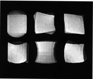
-normally have low-order modes which are intuitive to humans: bending, pinching, tapering, scaling, twisting, and shearing. Some of the low-order mode shapes for a cube are shown in Figure 2-3. Bodies with very dissimilar dimensions, or which have holes, etc., can have very complex low-frequency modes.

The bandwidth advantages of using such a parametric representation can be enormous. In a typical case in my system, the complete parametric representation of shape and nonrigid behavior requires only 120 bytes, whereas the vertex, polygon and normal representation with no non-rigid behavior information requires at least 4704 bytes.

Figure 2-3: A few of the vibration mode shapes of a 27 node isoparametric element.

2.2.2 Combination with Implicit Function Geometry

A further advantage is that such parametric representations may be combined with an implicit function surface to obtain extremely efficient collision detection [31, 24, 8]. In object-centered coordinates r = [r, s, t}T, the implicit equation of a spherical surface is

f(r) = f(r, s, t) = r2 _{+ s}2 _{+ t}2 _{- 1.0 = 0.0 (2.6)}

This equation is also referred to as the surface's inside-outside function, because to detect contact between a point X, = [X,, 1,, Z,]T and the volume bounded by this surface, one

simply substitutes the coordinates of X into the function

f.

A solid defined in this way can be easily positioned and oriented in global space, by transforming the implicit function to global coordinates, X = [X, Y, Z]T we get [31]:

where R is a rotation matrix, and b is a translation vector. The implicit function's positioned and oriented (rigid) inside-outside function becomes (using Equation 2.7):

f(r) = f(R~-'(X - b)). (2.8)

Any set of implicit shape functions can be generalized by combining them with a set of global deformations D with parameters m. For particular values of m the new deformed surface is defined using a deformation matrix Dm:

X = RDmr + b (2.9)

In my system the deformations used are the modal shape polynomial functions, defined by transforming the original finite element shape functions to the modal coordinate system (see [28]). These polynomials are a function of r, so that Equation 2.9 becomes:

X = REm)11 (r)r + b (2.10)

Combining the non-rigid deformation of Equation 2.10 with this inside-outside function we obtain,

f(r) = f(D-'(r)R-'(X - b)) (2.11)

This inside-outside function is valid as long as the inverse polynomial mapping D-1 (r) exists. In cases where a set of deformations has no closed-form inverse mapping, Newton-Raphson and other numerical iterative techniques have to be used.

This method of defining geometry, therefore, provides an inherently more efficient mathe-matical formulation for contact detection than geometric representations such as polygons or splines.

2.2.3 Additional Considerations for Displaying Graphics

Virtually all modem 3-D graphics libraries, such as the Programmer's Hierarchical Interactive Graphics System (PHIGS/PHIGS+), have only simple linear transformation capabilities, in order to allow for translation, scaling and perspective viewing of scenes composed of rigid objects. Because these library standards are optimized for storing static objects in a fixed display list they are poorly suited to the task of interactively displaying non-rigid simulations. Consequently, when using Equation 2.10, the entire vertex/polygon representation of all moving objects must be uploaded from the simulation engine into the graphics display list at each frame update.

But by considering only the whole-body deformations which are not functions of r, namely those of linear scale and shear, one is able to, as in Equation 2.9, compose a single 4x4 transformation matrix describing both the rigid and non-rigid motion of the simulated object. This allows one to preload the object's undeformed shape r into the display list, and obtain impressively fast displays of non-rigid dynamic simulation using standard graphics software and hardware.

To accomplish this the object's parameters of deformation is restricted to be

M = [Scaler, Scaley, Scale2 , Shear,, Shear,, Shear2] giving the deformation matrix,

Scale, Shear. Shear,

D = Shear2 Scale., Shear, . (2.12)

Sheary Shearx Scale,

This restricted deformation matrix also simplifies the computation necessary for collision detection in Equation 2.11, because the object's global inverse deformation matrix D- I (r) is a single matrix that is not dependent on r.

2.3 Bounded Asynchronous Operation

Synchronizing physical simulations of heterogeneous objects and situations intrinsically re-quires wasting a substantial amount of network bandwidth and CPU processing time. This is because each processor must wait until every other processor has broadcast its results the pre-vious time step before it can begin processing the next. Consequently, it is extremely desirable to allow some sort of asynchronous operation.

In the following, synchronous and asynchronous operation modes are mathematically an-alyzed by proving that the operation of an asynchronous network is equivalent to that of a particular type of synchronous network whose update rule considers the Hessian of the energy function. This result will then allow a formulation of a type of bounded asynchronous operation that results in faster and more stable network performance.

2.3.1 Energy Minimization

Physical simulation can be stated as a energy minimization problem. A time-varying three-dimensional potential field is defined by the sum of gravity, collisions, internal elasticity and damping, as well as the artificial potentials contributed by user-defined constraints. Objects act to minimize their potential energy by descending along the gradient of this potential energy surface.

Designating the system state by the vector U

(T)

U(T) = -VuE(U(T)) (2.13)

The system's state parameters "roll" down this energy surface until a collision occurs or a local minimum or "rest state" is reached. When a collision occurs, the potential energy surface warps in response to the new forces acting upon the colliding objects. The state parameters of these objects then begin to evolve along the new gradient direction.

the energy gradient of the entire physical system as a function of its parameters U at each time step, and then iteratively update the system parameters along the gradient direction by an amount proportional to the product of the gradient magnitude and the time step. If A.T is kept sufficiently small, then the true gradient direction will be accurately tracked and the simulation will accurately mimic the behavior of a real physical system.

2.3.2 Equivalent Operation Mode

In the preceding I assumed synchronous operation where the system state U(Ti) is updated at each time Ti+I = T + A T , for example,

U(T+1) = U(Ti) + AU(T) (2.14)

where

AU(Ti) = -Vu-E(,U(Tj))A T (2.15)

In asynchronous operation, each processor broadcasts the state changes of the objects it is simulating as soon as it has finished a time step. Thus each processor will receive state changes from other processors during each time interval A T. To describe asynchronous operation, therefore, the time interval A T is further divided into K smaller steps t1, such that

t1+1 = t, + A t where

At

U(Tj+1) = U(T) + AU(T) , (2.16)

where U and AU are now the time averaged update equation, which is related to the detailed behavior of the network by the relations

K

A U(T + tI-1 ) = -VUE(U(Tj + ti_1))At

and

U(Tj + ti) = U(Tj + ti_1) + AU(T + t 11 ) . (2.19)

Equations (2.16) to (2.19) describe "micro-state" updates that are conducted throughout each interval Tj whenever the gradient at subinterval t, is available, that is, whenever one of the network's processor's broadcasts the state changes of the objects that it is simulating.

2.3.3 Synchronous Equivalent to Asynchronous Operation

First, define the gradient and Laplacian of E at asynchronous times t, to be

Ai = VUE Br = V2E (2.20)

U=U(t1) U=U(tt)

and define that all subscripts of A, B, and t are taken to be modulo K.

Next, note that the gradient at time t 1 can be obtained by using the gradient at time Il and

Laplacian at times ti ... t, as below:

Ai+ = Ai

+

= I - /A tBI) Al (2.22)

H I - i/A tBk) A1 . (2.23)

k=1\

Assuming that A T is small, and thus that

At

1 K

VUE

-

U=U(T,) _{K 11}

K ~P K1 (1I - 7/ At (Bk) A1 (2.25) 1=1 k=1 t-/A _{(I -} T _{B) Ai (2.26)} 2 = I - TVE U=UT,))A1 . (2.27)

Thus the time-averaged state update equation for an asynchronous network is

U- - V2E _{A1 . (2.28)}

di U=U(T.) 2 U=U(T,)

This update function is reminiscent of second-order update functions which take into account the curvature of the potential energy surface by employing the Hessian of the potential energy

function [4]:

dUU

-- = -i;(I + pVjE-'VUE (2.29)

dT

where the identity matrix I is a "stabilizer" that improves performance when the Laplacian is small.

Taking the first-order Taylor expansion of equation (2.29) about V2 E = 0, dIU

-- ~ -r/(I - pVJE)VUE _(2.30)

dT II V

is obtained, and setting p = rIAT/2 equations (2.28) and (2.29) are shown to be equivalent

(given small A\T so that the Taylor expansion is accurate).

Thus equation (2.30) is a synchronous second-order update rule that is identical to the time-averaged asynchronous update rule of equation (2.28). This proves that the bounded asynchronous operation of such networks using a gradient update rule is equivalent to using a synchronous second-order update rule that considers the Hessian of the potential energy function.

enough, so that the approximations of equations (2.26) and (2.30) are valid. This condition is required of any physical simulation.

The second condition maintained is of bounded asynchrony: all parameters U must be updated once (on average) during every interval A T. The assumption of bounded asynchrony, however, requires distributing the computational load so that each object's behavior is, on average, being simulated at the same rate. Such resource allocation is a difficult problem in its own right, and is addressed in the following section.

2.4 Resource Allocation

Most systems which allocate tasks among multiple processors are based on some sort of cost-benefit analysis. Often such analyses require solving difficult nonlinear optimization problems. In recent years, however, simple distributed systems that use simple, localized mechanisms such as price, trade, and competition have been found to provide surprisingly good performance. Such systems are dubbed agoric systems for the greek word agora meaning market place [22]. Agoric systems are able to combine local decisions made by separate agents into globally effective behavior. These market-based ideas work because they do not attempt to formulate the "golden rule," or the "perfect loop," instead they set up a Computational Ecology [15], in which the simultaneous decisions of multiple and remote rational actors to converge on a global behavior that is for the common good.

A simple yet powerful example of such a system is the Enterprise system [20]. This system treats idle processors as contractors, and those requesting assistance as clients. Clients broadcast requests for "bids" from contractors on executing specific tasks. These requests contain information about the size and nature of the task at hand. A process server evaluates this information given its ability to handle tasks and replies with a bid corresponding to the estimated completion times for the task, and in a sense conveys the localized price that the client would actually pay for choosing that processor for that task.

wants to work with others in the colony to complete an infinite series of physical simulation iterations. Each iteration is completed with an integral amount of work from each contractor, and must be completed roughly within the global time interval AT in order to maintain the condition of bounded asynchrony.

If the ith processor is lagging behind others, so that the time AT' for that processor to complete an iteration of the simulation loop is longer than the average, then the condition of bounded asynchrony is jeopardized. Such delinquent processors must give part of their workload to processors that have below-average completion times, so that the simulation will not fall too far out of lock-step.

To determine whether they are delinquent and how much work they need to offload, all processors compare their iteration timing with the average iteration timing of all processors involved. If a processor P has an average elapsed timing that is greater than the average, it will try to offload a fraction Wt" of its own work to others where,

iAT' - AT a

W = .. (2.31)

But to which processor does this extra work go? And how can one processor offloading work be sure that it is not inadvertently combining with another offloading processor to overburden a below average processor? The key idea behind Huberman's [15] work is that there is no easy answer to these questions. They are the wrong questions, as they assume the existence of some perfect answer or "golden rule." A far more effective and elegant solution is to do something

simple now, and then again later if needs be.

In this spirit, my system offloads work at any one interval only to the processor P"," with the lowest timing (i.e., the one with the most time to spare). One must, however, be conservative about this: suppose that P"'" was the only processor with a below-average timing and all other processors P' have above-average timings. In this case every Pt will transfer some work to

of other processors (N - 2) to obtain the the percentage of work

W( = (2.32)

A Ti(N - 2)

that each above-average P' should give to P".

To execute this rule each timestep the processor needs to know only how many objects it is currently simulating, their relative computational cost, and the timings of the other processors. The timings can be easily transferred along with the object updates, adding negligible network bandwidth and communications overhead.

2.5

Experimental Results

This system has been implemented in C, and runs on DECStation 5000/200 and Sun 4 work-stations. The user interface processes are separate C processes and are derived from the ThingWorld modeling system [24, 26, 31, 8]. The underlying network code layer handling connections, byte swapping, and client/server requests is similar to that found in the X Win-dow System. This method was chosen because of its familiarity to users, and because of its demonstrated portability and efficiency.

2.5.1 Performance versus Number of Processors

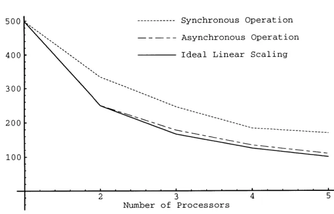
Graphs 2-4 and 2-5 show timings from the physical simulation of the non-rigid dynamics of 25 objects, including collision detection and response characterization. Twelve modes of deforma-tion were used for each object, and each object's geometry consisted of 360 polygons and 182 vertices. Also included were some point-position and point-to-point-attachment constraints on the objects being simulated.

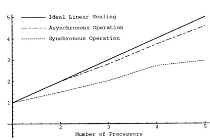
Figure 2-4 shows the elapsed time for 500 time steps of the physical simulation as a function of the number of processors used and the mode of operation (synchronous versus asynchronous versus ideal scaling). This data is replotted in Figure 2-5 to illustrate speedup of the physical

Elapsed Time (Seconds)

500 Synchronous Operation

Asynchronous Operation

400 Ideal Linear Scaling

300

200

---100

2 3 4 5

Number of Processors

Figure 2-4: Non-rigid physical simulation execution times versus the number of processors used in the simulation

Amount of Speedup

(2x, 3x...)

5 Ideal Linear Scaling Asynchronous Operation 4 --- Synchronous Operation

3

2 3 4 5

Number of Processors

Figure 2-5: The same timings expressed as the amount of speedup achieved in the simulation codes by adding additional processors.

simulation versus number of processors.

In this experiment all the processors were of the same type (DECStation 5000/200 work-stations), to simplify comparison. Simulation timings do not include graphics rendering or object processing overhead, including non-rigid polygon mesh regeneration, z-buffer render-ing, and camera transformations, as these costs depend upon individual camera viewpoints and the specifics of the graphics hardware employed. Also, when graphics hardware and camera viewpoint are constant among processors involved, this overhead is constant for all processors, and can thus be subtracted off to better illustrate speedups gained in the physical simulation codes. The average graphics processing overhead in this example was 85.37 CPU seconds over the 500 time steps, so that total execution time for computing and displaying 500 time steps of

this physical simulation is the time graphed in Figure 2-4 plus 85.37 seconds.

As can be seen, when using an asynchronous update rule the simulation time decreases quite nicely as the number of processors increases. For comparison, the ideal linear scaling function - where total execution time is equal to 1/n times the single processor execution time - is plotted as a solid line in Figures 2-4 and 2-5. The measured performance of the asynchronous network is qualitatively similar to that of the ideal linear scaling function, with

increasing network overhead accounting for most of the differences between ideal and observed execution times.

For comparison, the dotted line in Figures 2-4 and 2-5 shows the performance using a

synchronous update rule. It can be seen that much worse performance was obtained. This

is due to increasing numbers of wait states occurring as more and more processors are added and synchronized, always waiting for the slowest processor to finish. In the current system synchronous performace plateaus between five and ten processors. Asynchronous operation does not suffer from this problem, as the additional wait states are not introduced as more processors are added.

2.5.2 Load Leveling and Task Migration

One of the most important characteristics of the system is its ability to adapt to variable system loading. Such variable loading can occur because of user input (e.g., adding a new object), or collisions, or events external to the system (e.g., other users running jobs on the same processor). Whatever the cause, the system must quickly adapt its load distribution in order to maintain the condition of bounded asynchrony.

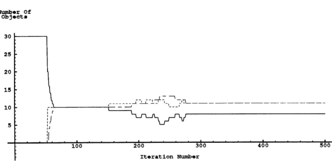
Figures 2-6 and 2-7 show a case of load distribution of 30 like objects among three computer workstations. In this example each workstation is responsible for a physical simulation process and a user interface / graphics process. Figure 2-6 shows the number of objects being handled by each of the three workstations, and Figure 2-7 shows the time each workstation requires to simulate one time step for all of its objects.

This example simulation starts by adding all 30 objects to one processors list and runs for 500 timesteps. In this example the resource allocation code is not activated until the 50th timestep; when it is engaged the three processors quickly (within five to ten iterations) equalize their workloads using the allocation scheme described above.

Sometime around the 1 5 0th iteration a command to spawn a new, outside, process was typed into a shell on the processor represented by the solid line. By the 2 5 0th iteration, the new

Number Of Objects 30 25 20 15 10 -' Iteration Number

Figure 2-6: Number of objects being simulated by each processor during task migration

Seconds Per Iteration 0.8 0.6 0.4 0.2 Iteration Number

the changes in actual workstation processor load. While the system was paging and spawning the new process, the processor affected acted independently to adjust the three workloads accordingly for the remainder of the simulation. The allocation scheme works similarly well in a variety of other configurations.

2.6 Examples

This section illustrates three examples of the modeling situations possible using the system described above. All of the simulations shown below were computed at interactive rates (i.e.

10-20 physics iterations/second).

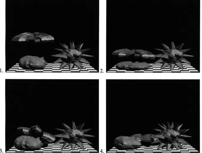
In the first example, a simple human figure is modeled using ten rigid superquadrics and nine point-to-point energy constraints. Shown in figure 2-8 is the system's response when the constraint holding up the head is deleted and the human model undergoes the transition between two rest states. Each superquadric is represented by 48 polygons with the exception of the head which has a higher sampling between 200 and 300 polygons.

In the second example, shown in figure 2-9, the system computes the rest state of a two dimensional 5x5 lattice of various superquadric objects strung together with energy constraints, and its rest state after twelve of the constraints are deleted. Again, each superquadric is represented by 48 polygons.

The third example shows the non-rigid response of 3 generalized superquadrics to object-object and object-object-floor collisions. Each superquadric in this example is sampled at between 200 and 300 polygons. See figure 2-10 and note how the spiked model rests on its spikes when sitting on the floor.

2.7 Summary

I have presented a system for distributed interactive simulation of complex, multi-body situa-tions using either rigid or non-rigid dynamics. The system's efficiency has been demonstrated

1. ~2.

3. 4.

1.

2.

3. - - -4

to increase significantly as a function of the number of processors, up to five processors, the maximum number tested. The system makes use of a novel bounded asynchronous operation mode allowing it to more fully utilize processor and network resources. It maintains this effi-ciency by allocating computational resources among networked workstations using a simple, efficient "market-based" strategy, thus avoiding problems of central control.

Chapter 3

Synchronization of Input and Output

In the preceeding chapter I addressed the problem of reducing the CPU time necessary to produce dynamic simulations of non-rigid objects. This reduction, although necessary, is not enough to ensure the synchronization of user motion and corresponding system response. Even in systems which simply mimic the sensor inputs with rendered graphical output, sufficient lag exists to muddle the synchrony and destroy the impression of realism.

This chapter proposes a suite of methods for accurately predicting sensor position in order to more closely synchronize processes in distributed virtual environments. An example system named MusicWorld employing these techniques is described.

Problems in synchronization of user motion, rendering, and sound arise from three basic causes. The first cause is noise in the sensor measurements. The second cause is the length of the processing pipeline, that is, the delay introduced by the sensing device, the CPU time required to calculate the proper response, and the time spent rendering output images or generating appropriate sounds. The third cause is unexpected interruptions such as network contention or operating system activity. Because of these factors, using the raw output of position sensors often leads to noticeable lags and other discrepancies in output synchronization.

Unfortunately, most interactive systems use raw sensor positions, or they make an ad-hoc attempt to compensate for the fixed delays and noise. A typical method for compensation averages current sensor measurements with previous measurements to obtain a smoothed

estimate of position. The smoothed measurements are then differenced for a crude estimate of the user's instantaneous velocity. Finally, the smoothed position and instantaneous velocity estimates are combined to extrapolate the user's position at some fixed interval in the future.

Problems with this approach arise when the user either moves quickly, so that averaging sensor measurements produces a poor estimate of position, or when the user changes velocity, so that the predicted position overshoots or undershoots the user's actual position. As a consequence, users are forced to make only slow, deliberate motions in order to maintain the illusion of reality.

A solution to these problems is presented which is based on the ability to more accurately predict future user positions using an optimal linear estimator and on the use of fixed-lag dataflow techniques that are well-known in hardware and operating system design. The ability to accurately predict future positions eases the need to shorten the processing pipeline because a fixed amount of "lead time" can be allotted to each output process. For example, the positions fed to the rendering process can reflect sensor measurements one frame ahead of time so that when the image is rendered and displayed, the effect of synchrony is achieved. Consequently, unpredictable system and network interruptions are invisible to the user as long as they are

shorter than the allotted lead time.

3.1 Optimal Estimation of Position and Velocity

At the core of this technique is the optimal linear estimation of future user position. To accomplish this it is necessary to consider the dynamic properties of the user's motion and of the data measurements. The Kalman filter [17] is the standard technique for obtaining optimal linear estimates of the state vectors of dynamic models and for predicting the state vectors at some later time. Outputs from the Kalman filter are the maximum likelihood estimates for Gaussian noises, and are the optimal (weighted) least-squares estimates for non-Gaussian noises [9].

translational components (the x, y, and z coordinates) output by the Polhemus sensor, and to assume independent observation and acceleration noise. This section, therefore, will develop a Kalman filter that estimates the position and velocity of a Polhemus sensor for this simple noise model. Rotations will be addressed in the following section.

3.1.1 The Kalman Filter

Let us define a dynamic process

Xk+1 = f(Xk, At)+ ((t) (3.1)

where the function f models the dynamic evolution of state vector Xk at time k, and let us define an observation process

Yk = h(Xk, At) + r;(t)

(3.2)

where the sensor observations Y are a function h of the state vector and time. Both ( and qj are white noise processes having known spectral density matrices.

In this case the state vector Xk consists of the true position, velocity, and acceleration of the Polhemus sensor in each of the x, y, and z coordinates, and the observation vector Yk consists of the Polhemus position readings for the x, y, and z coordinates. The function f will describe the dynamics of the user's movements in terms of the state vector, i.e. how the future position in x is related to current position, velocity, and acceleration in x, y, and z. The observation function h describes the Polhemus measurements in terms of the state vector, i.e., how the next Polhemus measurement is related to current position, velocity, and acceleration in x, y, and z.

Using Kalman's result, one can then obtain the optimal linear estimate Xk of the state vector

Xk by use of the following Kalman filter:

Xk = X* + Kk(Yk - h(X*, t)) (3.3)

algorithm uses a state prediction X*, an error covariance matrix prediction P*, and a sensor measurement Yk to determine an optimal linear state estimate Xk, error covariance matrix estimate Pk, and predictions X* 1 , P*I for the next time step.

The prediction of the state vector X*i at the next time step is obtained by combining the optimal state estimate Xk and Equation 3.1:

X+I = Xk + f(Xk, iAt)At (3.4)

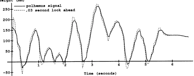
In my graphics application this prediction equation is also used with larger times steps, to predict the user's future position. This prediction allows synchrony with the user to be maintained by providing the lead time needed to complete rendering, sound generation, and so forth.

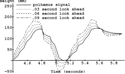
Calculating The Kalman Gain Factor

The Kalman gain matrix Kk minimizes the error covariance matrix Pk of the error ek =

Xk - Xk, and is given by

Kk = P*Hk T(HkP*Hk T + R.~' (3.5)

where R = E[r,(t)p(t)T] is the n x n observation noise spectral density matrix, and the matrix Hk is the local linear approximation to the observation function h,

[Hk]l; = ahi/Ox, (3.6)

evaluated at X = X*.

Assuming that the noise characteristics are constant, then the optimizing error covariance matrix Pk is obtained by solving the Riccati equation

0=P* = FkP* + P*FT - P*HR -'1HkP* + Q (3.7)

Height (mm)

polhemus signal

250t- .03 second look ahead

Time (seconds)

Figure 3-1: Output of a Polhemus sensor and the Kalman filter prediction of that lead time of 1/30th of a second.

and Fk is the local linear approximation to the state evolution function f,

[Fklij = ofC/Ox

output for a

(3.8)

evaluated at X = Xk.

More generally, the optimizing error covariance matrix will vary with time, and must also be estimated. The estimate covariance is given by

Nk

From this the predicted error covariance matrix can be obtained

(3.10)

Pk+ = Ikpkek + Q

where #4 is known as the state transition matrix

i = (I

+

150 100.

-50.

3.1.2 Estimation of Displacement and Velocity

In my graphics application I use the Kalman filter described above for the estimation of the displacements Ps, P., and P, the velocities V7,

1,

Ay, and A, of Polhemus sensors. The state vector X of the dynamic system is therefore

(Px, Vx, Ax1, Py, Vy Ay, P2, V, A2)T, and the state evolution function is

f(X, At) = V" + Ax At Ax 0 Vy + Ay2 AY 0

V2

AA

The observation vector Y will be the positions Y = (P', P', P,')T that are the output of the Polhemus sensor. Given a state vector X the measurement using simple second order equations of motion is predicted: h(X, At) = + 1.At + Ax A" + V At+ A "" z ₂ (3.13)

Calculating the partial derivatives of equations 3.6 and 3.8 we obtain 0 1 0 0 1 0 0 1 0 and

Finally, given the time k + Ai by

1 t A₂ H1

state vector Xk at time k

2t (3.15)

1 At t

one can predict the Polhemus measurements at

Yk+At = h(Xk, At') (3.16)

and the predicted state vector at time k + A t is given by

Xk+At = Xk + f(Xk, At)At (3.17)

The Noise Model

I have experimentally developed a noise model for user motions. Although the noise model is not verifiably optimal, I find the results to be quite sufficient for a wide variety of head and hand tracking applications. The system excitation noise model

$