MIT Joint Program on the Science and Policy of Global Change
combines cutting-edge scientific research with independent policy analysis to provide a solid foundation for the public and private decisions needed to mitigate and adapt to unavoidable global environmental changes. Being data-driven, the Joint Program uses extensive Earth system and economic data and models to produce quantitative analysis and predictions of the risks of climate change and the challenges of limiting human influence on the environment— essential knowledge for the international dialogue toward a global response to climate change.
To this end, the Joint Program brings together an interdisciplinary group from two established MIT research centers: the Center for Global Change Science (CGCS) and the Center for Energy and Environmental Policy Research (CEEPR). These two centers—along with collaborators from the Marine Biology Laboratory (MBL) at
Woods Hole and short- and long-term visitors—provide the united vision needed to solve global challenges.
At the heart of much of the program’s work lies MIT’s Integrated Global System Model. Through this integrated model, the program seeks to discover new interactions among natural and human climate system components; objectively assess uncertainty in economic and climate projections; critically and quantitatively analyze environmental management and policy proposals; understand complex connections among the many forces that will shape our future; and improve methods to model, monitor and verify greenhouse gas emissions and climatic impacts.
This reprint is intended to communicate research results and improve public understanding of global environment and energy challenges, thereby contributing to informed debate about climate change and the economic and social implications of policy alternatives.
—Ronald G. Prinn and John M. Reilly, Joint Program Co-Directors
MIT Joint Program on the Science and Policy
of Global Change Massachusetts Institute of Technology 77 Massachusetts Ave., E19-411 Tglobalchange@mit.edu (617) 253-7492 F (617) 253-9845
December 2016
Economic Projection with Non-homothetic
Preferences: The Performance and
Application of a CDE Demand System
Economic Projection with Non-homothetic
Preferences: The Performance and Application
of a CDE Demand System
Y.-H. Henry chen
Abstract: In computable general equilibrium modeling, whether the simulation results are consistent to a set of valid own-price and income demand elasticities that are observed empirically remains a key challenge in many modeling exercises. To address this issue, the Constant Difference of Elasticities (CDE) demand system has been adopted by some models since the 1990s. However, perhaps due to complexities of the system, the applications of CDE systems in other models are less common. Furthermore, how well the system can represent the given elasticities is rarely discussed or examined in existing literature. The study aims at bridging these gaps by revisiting calibration details of the system, exploring conditions where the calibrated elasticities of the system can better match a set of valid target elasticities, and presenting strategies to incorporate the system into GTAP8inGAMS—a global computable general equilibrium model written in GAMS and MPSGE modeling languages. It finds that the calibrated elasticities can be matched to the target ones more precisely if the corresponding sectorial expenditure shares are lower, target own-price demand elasticities are lower, and target income demand elasticities are higher. It also verifies that for the GTAP8inGAMS with a CDE system, the model responses can successfully replicate the calibrated elasticities under various price and income shocks.
1. INTRODUCTION ...2
2. THEORETICAL BACKGROUND ...3
2.1 reGULArITY AND FLeXIbILITY OF A DemAND SYSTem ...3
2.2 THe cDe DemAND SYSTem ...4
3. CALIBRATION, PERFORMANCE, AND IMPLEMENTATION...4
3.1 cALIbrATION ...5
3.2 PerFOrmANce ...5
3.3 ImPLemeNTATION ...8
4. CONCLUSION ... 12
5. REFERENCES ... 13
APPENDIX A: THE CDE CALIBRATION PROGRAM ... 14
APPENDIX B: THE CGE MODEL WITH CDE DEMAND FOR GTAP8INGAMS ...17
APPENDIX C: THE PROGRAM CHECKING IF ELASTICITY TARGETS ARE VALID ...21
1. Introduction
In Computable General Equilibrium (CGE) modeling, it has been identified that price and income elasticities of demand are crucial in determining the sectorial growth pattern and economic impacts of various policies (Her-tel, 2012). This suggests that while a typical Constant Elasticity of Substitution (CES) function is still widely used in modeling final consumption (Sancho, 2009; An-nabi et al., 2006; Elsenburg, 2003), the property of having unitary income elasticities of demand is often considered as highly inflexible. Also, in a single-nest CES setting, af-ter applying the Cournot’s aggregation, it can be shown that the sectorial expenditure shares will fully determine the variation in own-price elasticities of demand, which is quite restrictive as well.
To capture the observed non-homothetic preferences with income elasticities of demand diverging from uni-ty, one approach is to use the Linear Expenditure System (LES) such as the Stone-Geary preference (Geary, 1950; Stone, 1954). The LES system can be calibrated to income elasticities of demand compatible to a valid demand sys-tem. In addition, with a special multi-nest structure, the calibrated own-price elasticities of demand can be matched perfectly to any valid elasticities (Perroni and Rutherford, 1995).1 The shortcoming of LES, however, is
that due to constant marginal budget shares with respect to income, the limit property of LES is still constant-re-turn-to-scale, and therefore the underlying income elas-ticities of demand will approach one as income grows. An alternative option to model non-homotheticity is to utilize the Constant Difference of Elasticities (CDE) de-mand system proposed by Hanoch (1975). With implicit additivity, a N-commodity CDE system has N expansion parameters and N substitution parameters to achieve a more general functional form than the single nest CES case. The N expansion parameters make it possible to in-corporate various income elasticities of demand across commodities/sectors, and the income elasticities will re-main at their given levels as income changes (“commod-ity” and “sector” are used interchangeably in this study). On the other hand, compared to a single-nest CES set-ting, the N substitution parameters allow modelers to come up with a somewhat better representation for the target own-price demand elasticities.
One caveat of CDE applications, paradoxically, comes from the constancy of each income elasticity regardless of income levels. While this feature might not severely contradict empirical evidence for developed countries, 1 While Perroni and Rutherford (1995) focuses on homothetic pref-erences, it points out that the multi-nest strategy achieving a perfect match in own-price elasticities calibration also works for non-homo-thetic preferences.
existing studies have found that, for instance, income elas-ticities of some food items in developing countries tend to decrease as income grows (Haque, 2005; Chern et al., 2003). In some cases, economic growth may turn luxury goods into necessities (Zhou et al., 2012). To overcome this, with more income response parameters, Rimmer and Powell (1996) presents an implicit directly additive de-mand system (AIDADS) that allows income elasticities of demand to vary logistically. Nevertheless, AIDADS has a narrow range of substitution across goods, and due to the-oretical and computational reasons, AIDADS applications are limited to 10 commodities/sectors (Reimer and Hertel, 2004). As a result, these applications are less common and more project-specific. In contrast, despite some limita-tions, the CDE system seems to be more applicable as a generic setting for modeling non-homothetic preferences. While CGE models such as GTAP (Hertel and Tsigas, 1997), MAGNET (Woltjer and Kuiper, 2014), GTEM (ABARE/DFAT, 1995; ABARE, 1996), and ENVISAGE (van der Mensbrugghe, 2008) have been using CDE sys-tems in modeling final consumption behaviors, perhaps due to the complexities in both calibration and imple-mentation, other CDE applications are less common so far. More importantly, when studying the responses of CGE models with non-homothetic preferences, besides examining the implications of income elasticities of de-mand on future projection, the roles of own-price elas-ticities of demand are crucial as well, since own-price demand elasticities could also influence projections and may become even more crucial under some policy shocks. Existing literature also points out that to ensure the regularity of a well-behaved demand function, cal-ibrating a CDE system to the target elasticities that are valid might be infeasible (Hertel, 2012; Huff et al., 1997). How well the system can match those elasticities is be-yond the discussion of most existing literature. One ex-ception is Liu et al. (1998), which presents the differences between target and calibrated elasticities. Nevertheless, exploring sources of differences between calibrated and target elasticities is beyond the scope of that study. Before studying how well the calibrated elasticities of a demand system can match a set of target elasticities, one needs to ensure that under a given baseline expenditure share structure, the target elasticities are valid, i.e., they are conformable to aggregation conditions and a negative semi-definite Slutsky matrix. Therefore, the demand sys-tem under consideration will only be calibrated to a set of valid target elasticities. With that in mind, the study will answer the question both analytically and numerically: given a set of valid target own-price demand elasticities, income demand elasticities and expenditure shares, under what conditions will the calibrated elasticities of a CDE system better match the target values? The findings of this
study can help modelers who implement a CDE system explaining how well the target elasticities are represented in their models, and provide information for choosing an appropriate sectoral aggregation so that, if possible, at least target elasticities of interesting sectors can be better matched. Next, the author presents strategies for putting the CDE system into GTAP8inGAMS, a global CGE mod-el written in GAMS and MPSGE using the GTAP 8 data-base (Rutherford, 2012). MPSGE is a subsystem of GAMS (Rutherford, 1999), and earlier it was sometimes thought that despite being a powerful tool that handles the calibra-tion of CES funccalibra-tions automatically, MPSGE can only be applied to models with CES or LES utility functions (Kon-ovalchuk, 2006; Hertel et al., 1991). The study shows that the potential of MPSGE applications is far beyond what was previously perceived. The revised GTAP8inGAMS with a CDE system is tested with income and price shocks to verify the model response is consistent to the calibrated elasticities. The programs for the CDE calibration and the revised GTAP8inGAMS with a CDE system are provided in Appendix A and Appendix B, respectively, so readers can use them for verification or research purposes. The rest of the paper is organized as follows: Section 2 briefly reviews the theories and settings of the CDE sys-tem; Section 3 presents the calibration, performance, and implementation of the CDE system; and Section 4 pro-vides a conclusion.
2. Theoretical Background
To understand what constitutes a regular (i.e., valid) de-mand response, the section will briefly review the econom-ic considerations for a regular demand system. A question that follows is: how can one evaluate the performance of a regular demand system in terms of representing the target own-price and income demand elasticities that are valid? To explore this, the section will discuss a demand system’s flexibilities in own-price and income demand elasticities calibration, introduce the settings of CDE system, and fi-nally examine the implications of CDE regularity condi-tions on the calibration performance of the system. 2.1 Regularity and Flexibility of a Demand
System
Let us denote a cost (or expenditure) function by C(p,u) where p is a N-dimensional price vector and u is the utility. For C to be considered as well-behaved, ∂C/∂p, which is the Hicksian demand vector q(p,u), is non-negative and homogeneous of degree zero in p, and [∂^
2
C/∂p_(i)∂p_(j) ]_(N×N), which is the Slutsky matrix, is negative
semi-definite (NSD).2 The intuition of a NSD Slutsky
ma-trix is: for a given utility level u, when a good becomes 2 For example, see p.59 and p.933 in Mas-Colell et al. (1995).
more expensive, it will be replaced by other cheaper al-ternatives; as a result, the cost increase with the new con-sumption bundle after the price increase will never ex-ceed the cost increase when the bundle cannot be altered. The Slutsky matrix [∂^
2C/∂p
_(
i)∂p_(j)]_(N×N), or
equivalent-ly [∂q/∂p]_(N×N), is symmetric and each term of the
matrix is:
(1) Equation (1) is the Slutsky equation, which decompos-es the impacts of a price change on the uncompensated demand x_(i)(p,w) into the income effect and
substitu-tion effect, where w is the income (or expenditure) lev-el. With some algebra, the Slutsky equation can also be expressed as (2) where σ_(ij)^( c ) , σ_(ij)^( m, η
_(i), and θ_(j) are compensated price
elastic-ity of commodelastic-ity i, uncompensated price elasticelastic-ity of i, income elasticity of i, and expenditure share of j, re-spectively. If both sides of (2) are divided by θ_(j), one can
come up with a Slutsky matrix [σ_(ij) ]_(
N×N in the form of
Allen-Uzawa elasticity of substitution (AUES) (Allen and Hicks, 1934; Uzawa, 1962) with
(3) It can be shown that [σ_(ij) ]_(
N×N is also symmetric, and the
matrix is NSD if and only if [∂q/∂p]_(N×N) is NSD.
There-fore, a demand system is regular means 1) the Slutsky matrix [σ_(ij) ]_(
N×N) is NSD; and 2) the Hicksian demand
q is non-negative. For CGE modeling, it is necessary to ensure that the demand system is globally regular (i.e., it should remain regular everywhere in the domain of price). This is because the algorithm of the solver for finding equilibria may begin from an initial point of price and quantity combination that is far from the equilibri-um levels, and in the process of solving the model, the algorithm might fail if the demand system is not globally regular, even the system is locally regular at the equilibri-um points (Perroni and Rutherford, 1998).
Perroni and Rutherford (1995) defined a regular-flexible demand system as the one that is globally regular and can locally represent any valid configuration of compensated demands and the AUES matrix [σ_(ij) ]_(
N×N. Based on an
inductive argument, Perroni and Rutherford proved that a demand system derived from a special version of the non-separable nstage CES function is regular-flexible. Nevertheless, in general, testing whether other demand systems are regular-flexible would need to identify the domain of a regular flexible demand system first, which
is beyond the scopes of their paper and the current re-search. Instead of matching the entire AUES matrix under a given expenditure share structure, this study will simply focus on the ability of a demand system in matching a valid combination of ownprice elasticities, income demand elasticities, and expenditure shares. Own-price and income elasticities are usually of first-or-der importance in characterizing the model response, and are also the most ubiquitous data available for cal-ibrating a demand system. In particular, this study will examine whether a global regular demand system under consideration is own-price and income flexible (i.e., if the system can be calibrated to (σ_(ii), η_(i), θ_(i)) consistent
to any well-behaved cost function). Following this defi-nition, for example, the demand system derived from a single-nest CES cost function is neither own-price nor income flexible. The settings of CDE and their implica-tions on own-price and income flexibilities will be dis-cussed below.
2.2 The CDE Demand System
Let us consider the expenditure function C with a price vector p and a Hicksian demand vector q, i.e., c_(0)=C(p_(0),u)≡{minp_(0)q_(0):f(q_(0))≥u} where the
sub-script 0 denotes the benchmark condition. If the func-tion is normalized by c_(0), it becomes C(p_(0)/c_(0),u)≡1.
With this normalization, Hanoch (1975) proposes the ex-penditure function of a CDE demand system as follows:
(4) where α_(i) and e_(i) are the substitution parameter and
ex-pansion parameter, respectively. In this setting, the utility u is only implicitly defined, and in general there is no re-duced form representation for u. The Hicksian demand for commodity i based on this setting is:
(5)
For the CDE system, the substitution elasticity σ_(ij) in
AUES form is presented in Equation (6), where the ex-penditure share is denoted by θ_(i), and δ_(ij)=1 if i=j,
oth-erwise δ_(ij)=0. The income elasticity of demand η_(i) is
pre-sented in Equation (7):
(6)
(7)
The following aggregation conditions hold: the Cournot’s aggregation ∑_(i)θ_(i)σ_(ij )=0 and the Engel’s aggregation
∑_(i)θ_(i)η_(i) =1. Note that for each off-diagonal term,
σ_(ij)-σ_(ik)=αj_()-α_(k) is invariant to i although σ_(ij) may vary,
and therefore the system has a constant difference of (substitution) elasticities. The regularity condition for the system presented in Hanoch (1975) includes: β_(i) ≥0;
e_(i) ≥0; 0<α_(i <1 or α) _(i) ≥1∀i and α_(I) >1 for some I ∈ i.
It is worth noting that with the regularity condition, each own-price elasticity of demand σ_(ii)^(
c
)
is always negative. This is because from Equation (6) and σ_(ii)^(
c
)
=σ_(ii)θ_(i), we have (8) For a given vector of θ_(i), the requirement that all α_(i)s
should lie on the same side of one imposes a constraint in choosing the vector of α_(i) such that σ_(ii)^(
c
)
can match the target own-price demand elasticity. For instance, some sectors may have a very small expenditure share (θ_(i)→0)
and so for those sectors σ_(ii)^(
c
)
→-α_(i). However, for those
sectors, if some target own-price elasticities do not lie on the same side of one, it would be impossible to match every single σ_(ii)^(
c
)
with the target elasticity value no mat-ter what regulatory condition on α_(i) is chosen. Therefore,
the CDE system is not own-price flexible. Further, the requirement of e_(i) ≥0 also suggests that some
compro-mise has to be made in calibrating income elasticities of demand.
3. Calibration, Performance, and
Implementation
Two CDE calibration approaches have been presented. The first is the three-step procedure documented in Her-tel et al. (1991) and Huff et al. (1997). In this approach, own-price demand elasticities are calibrated to target lev-els first. Taking parameters determined in the first step as given, income elasticities of demand are calibrated to target levels next, and scale parameters of the system are specified last. The second method is the maximum en-tropy approach presented by Surry (1997) and Liu et al. (1998). Rather than calibrating the system sequentially, the idea of this approach is to calibrating all parameters simultaneously by maximizing an objective function that considers matching both own-price and income elastic-ities of demand. This study will take the first approach as an example and explore under what circumstanc-es the calibrated elasticiticircumstanc-es can better match the target elasticities, the section will examine the performance of CDE calibration both analytically and numerically. It will also demonstrate how to put the CDE system into GTAP8inGAMS and verify the model response is consis-tent to the calibrated elasticities.
3.1 Calibration
Step 1: Calibrating the own-price elasticity of demand
σiic ). Let us denote the target own-price elasticity of
de-mand by σ_(ii)^(
ct
)
. The purpose of this step is to choose α_(i)
so that the “distance” between the two vectors [σ_(ii)^(
c ) ] and [σ_(ii)^( ct )
] is minimized.3 In this study, the following function
is considered for the minimization problem:
(9)
where ω_(i)=θ_(i). The study will compare the performances
of different settings in matching the target own-price de-mand elasticities.
Step 2: Calibrating the income elasticity of demand. Let us denote the target income elasticity of demand by η)^(_(i
t
)
(η)^(_(i
t
) must satisfy the Engel’s aggregation). Given α_(i)
deter-mined in the previous step, by choosing e_(i), the goal is to
calibrate η_(i) to η_(i)^(
t
)
if possible. Similar to the idea of Step 1, the following problem is solved:
(10)
The condition ∑_(i)θ_(i)η_(i)=1 is to ensure the calibrated
elasticities satisfy the Engel’s aggregation, and following Huff et al. (1997), the second condition is to ensure the calibrated elasticities lie on the same side of one as the target values.
Step 3: Calibrating the scale coefficients holding the
util-ity level equals one. With the calibrated α_(i) and e_(i), and
the normalization u=1, p_(0i)=1, and q_(0i)=θ_(i) (since c_(0)
= ∑_(i)p_(0iq) _(0i) =1), the N scale parameters β_(i) can be solved
by using (4) and (5):
(11) Because the calibration is done sequentially, how well the income elasticities of demand can be matched to tar-get levels is also affected by the calibration of own-price demand elasticities. In Appendix A, the study provides the program for the three-step strategy. The program is written in GAMS, and each minimization problem in the program is formulated as a nonlinear programming (NLP) problem.
3 Without explicitly considering the distance metric, the objective function of this problem considered in Huff et al. (1997) is f(σ_(ii)^(
c ) )=∑_(i) σ_(ii)^( c ) [ln (σ_(ii)^( c ) /σ_(ii)^( ct ) ) - 1]. 3.2 Performance
Before putting the system into a CGE model, two inter-esting questions are: under what circumstances does the calibration become more accurate, and how well are the target elasticities represented? The following analysis will answer these questions.
Proposition 3.2.1:
The lower the expenditure share, the higher the influ-ence of own-sector substitution parameter in deter-mining the calibrated own-price elasticity of demand. On the other hand, the higher the expenditure share, the higher the influence of other sectors’ substitution parameters in determining the calibrated elasticity.
Proof: Since σ_(ii)^( c ) =-α_(i) (1- θ_(i) )^ 2- θ _( i) ∑_(k|k≠i)θ_(k)α_(k) , with a lower θ_(i) (θ_(i) ∈ (0,1)), σ_(ii)^( c )
depends more on the own-sector substitution parameter α_(i), rather than
the weighted average of other sectors’ substitution parameters ∑_(k|k≠i) θ_(k)α_(k) . In the extreme case with
θ_(i) →0, if the regularity condition is not violated,
σ_(ii)^(
c
)
can be matched to the target level σ_(ii)^(
ct ) by sim-ply setting α_(i)=-σ_(ii)^( ct ) since σ_(ii)^( c ) =-α_(i). On the
other hand, with a higher θ_(i), σ_(ii)^(
c
)
depends more on the weighted average of other sectors’ substitu-tion parameters ∑_(k|k≠i)θ_(k)α_(k) rather than the
own-sector substitution parameter α_(i). In the extreme
case with θ_(i)→1, α_(i) has no control over σ_(ii)^(
c ) since σ_(ii)^( c ) =∑_(k|k≠i)θ_(k)α_(k).
Since the compensated own-price elasticities of demand presented in GTAP 8 are between - 1 and 0, based on discussions above, considering the regularity condition with α_(i) ∈ (0,1) produces more accurate calibration
re-sults for sectors with smaller expenditure shares. With a higher sectorial resolution, more commodities/sectors will have smaller expenditure shares, and thus having α_(i) ∈ (0,1) will make it possible for producing a better
match between calibrated and target levels for each indi-vidual sector.
Proposition 3.2.2:
When α_(i) ∈ (0,1), calibrating the income
elastici-ty of demand to a higher level is less likely to violate
e_(i) ≥0, which is part of the regularity condition. On
the other hand, when α_(i) ≥1 ∀ i and α_(I) >1 for some
I ∈ i, calibrating the elasticity to a lower level is less
likely to violate e_(i) ≥0. Proof:
From Equation (7),
e_(i)={∑_(k)θ_(k)e_(k) [η_(i)-(α_(i)-∑_(kθ) _(k)α_(k))]-∑_(k)θk_()e_(k)α_(k)}/(1-α_(i)).
equation above is needed to ensure e_(i) ≥0.
There-fore, other things being equal, with a higher cali-brated income elasticity of demand η_(i), the
numer-ator is less likely to become negative. Similarly, for α_(i) ≥1 ∀ i and α_(I) >1, a lower η_(i) is less likely to
vi-olate e_(i) ≥0.
If one considers α_(i) ∈ (0,1), the second proposition
sug-gests that matching the target income elasticities for the demand of agricultural products might be trickier, since in general these products tend to have lower income elastic-ity values; as a result, the calibrated income demand elas-ticities for these products might end up with levels higher than the target numbers. Nevertheless, the values of α_(i)
de-termined in Step 1 of the calibration procedure may also affect how well the target income elasticities of demand are met, as will be explored in the next proposition. Proposition 3.2.3:
When α_(i) ∈ (0,1), calibrating the income
elastici-ty of demand to a target level is less likely to violate
e_(i) ≥0 with a smaller α_(i). On the other hand, when
α_(i) ≥1 ∀ i and α_(I) >1 for some I ∈ i, calibrating the
elasticity to the target level is less likely to violate e_
(
i) ≥0 with a larger α_(i). Proof:
This can be verified by e_(i)={∑_(k)θ_(k)ek_() [η_(i)- (α_(i)- ∑_(k)
θ_(k)α_(k) )]- ∑_(k)θ_(k)e_(k)α_(k) }/(1- α_(i)).
Continuing our previous example for commodities with low income elasticities of demand and with α_(i) ∈ (0,1), while Proposition 3.2.2 says that for
given values of α_(i), it is harder to calibrate the
in-come elasticity of demand to a lower value, Propo-sition 3.2.3 suggests that if the calibrated α_(i) is small
enough, it is still possible to calibrate the income elasticity of demand to a lower level.
Proposition 3.2.4:
Commodities with substitution parameters α_(i) close
to one will have similar calibrated income elasticities of demand.
Proof:
From Equation (7),
η_(i)=∑_(k)θ_(ke) _(k)α_(k)/∑_(k)θ_(k)e_(k)+1- ∑_(k)θk_( )α_(k)= η_(j).
Proposition 3.2.4 shows that the calibrated α_(i) may work
against the calibration for income elasticities of demand. For instance, if there are two commodities with α_(i) and
α_(j) both approaching unity, according to the proposition,
the calibrated income elasticities of demand η_(i) and η_(j)
will be very close to each other, even if their target values η_(i)^( t ) and η)^(_(j t )
are quite different.
To show how different sectorial aggregation levels could affect the accuracy of elasticity calibration, the study con-siders several different aggregation levels (Table 1).4 For
demonstration purpose, all GTAP regions are combined into a single region using the aggregation routine of GTAP8inGAMS. In particular, wherever needed, target elasticities are aggregated based on expenditure shares. It is worth noting that the 10-sector income demand elas-ticity estimates based on an implicit directly additive de-mand system (AIDADS) were mapped to and used as the target income demand elasticities of the original GTAP database, and following Zeitsch et al. (1991), income de-mand elasticities are then used to compute the own-price 4 For all settings, there is a single aggregated region and 2 aggregat-ed primary factors: labor and capital.
Table 1. Settings for calibration exercises with various sectorial aggregation levels. Aggregation Level # of
Sectors Settings
1r3s2f 3 Combine GTAP sectors 1–14 (g01–g14) & 22–26 (g22–g26) into s01 (agriculture); g15–g21 & g27–g46 into s02 (manufacturing); and g47–g57 into s03 (service). 1r4s2f 4 Similar to 1r3s2f, except the service sector is disaggregated into a trade and transport
sector (g47–g51) and a service sector (g52–g57).
1r5s2f 5 Combine g01–g17 into s01; g18–g27 into s02; …; g48–g57 into s05. 1r8s2f 8 Combine g01–g15 into s01; g16–g21 into s02; …; g52–g57 into s08.
1r16s2f 16 Combine g01–g12 into s01; g13–g15 into s02; g16–g18 into s03; …; g55–g57 into s16. 1r29s2f 29 Combine g01–g02 into s01; g03–g04 into s02; …; g55–g56 into s28; g57 becomes s29.
demand elasticities of the database, as documented in Hertel et al. (2014).
To assess the calibration performance for each type of elasticity, in addition to a one-by-one comparison be-tween calibrated and target numbers for each commod-ity, it is informative to have an index for measuring how far the point of calibrated elasticities is from the point of target elasticities as follows:
(12) Depending on the type of elasticity evaluated, x_(i) in
Equa-tion (12) could be either the own-price elasticity of de-mand σ_(ii)^(
c
)
or the income elasticity of demand η_(i), while
the superscript x_(i)^(
t
)
denotes target value and ω_(i)=θ_(i).
When the 57 GTAP sectors are aggregated into a 3-sec-tor setting, even the smallest sec3-sec-torial expenditure share, denoted by θ_(min), approximates 12%, and with this
set-ting the largest share θ_(max) exceeds 63%. As the
sectori-al resolution increases, the difference between θ_(max) and
θ_(min) is reduced. In the most disaggregated case where
all 57 GTAP sectors are kept, θ_(max) is slightly above 17%
and θ_(min) is only 0.0002% (Table 2). Per compensated
own-price demand elasticity targets, the range between the largest one σ^(
ct
)_(max) and the smallest one σ^(
ct
)_(
min) increases
as the sectorial resolution gets higher, since more disag-gregated setting means extreme values are more likely to appear. In general, σ^(
ct
)_(
max) becomes larger (|σ^(
ct
)_(
max)|
be-comes smaller, i.e., less elastic) and σ^(
ct
)_(
min) becomes smaller
(|σ^(
ct
)_(min)| becomes larger, i.e., more elastic) as the sectorial
resolution increases. The same story applies to the in-come demand elasticity targets—with more disaggregat-ed sectors, the range between η^(
ct )_( max) and η^( ct )_( min) increases as η^( ct )_(
min) becomes smaller (less elastic) and/or η^(
ct
)_(
max) becomes
larger (more elastic).When trying to calibrate the CDE system to the target own-price and income demand elas-ticities, it is important to verify if the target own-price demand elasticities are compatible to an AUES matrix that is NSD. For instance, with the 3-sector setting, based on the Cournot aggregation, the three off-diago-nal terms of the AUES matrix are fully determined once the own-price demand elasticities in AUES form (i.e., the diagonal terms of the matrix) are given, and hence the whole AUES matrix is identified. However, this will not be a valid AUES matrix since it is not NSD, which means the target own-price demand elasticities under the three-sector setting are invalid, and one cannot claim the CDE system is not flexible based on this setting. On the other hand, in the 4-sector, 5-sector, 8-sector, and 16-sector settings, it can be shown that under each set-ting, the target own-price demand elasticities are com-patible to an AUES matrix that is NSD, and therefore the target elasticities are valid. More specifically, if one
denote the number of sectors/commodities by n, there will be n∙(n- 1)/2 - n free variables that are off-onal terms in an AUES matrix. Therefore, once the diag-onal terms (compensated own-price demand elasticities in AUES form) are given, one can use random number generators to assign values for those off-diagonal terms (cross-price demand elasticities in AUES form), and then choose the combination that yields a NSD AUES matrix. The MATLAB subroutine for doing this job is presented in Appendix C.
Since with various sectorial aggregation levels, own-price demand elasticity targets are all between 0 and 1, to cal-ibrate the CDE system, similar to Huff et al. (1997), the study chooses α_(i) ∈ (0,1), a setting that produces a more
accurate own-price demand elasticity calibration when the sectorial resolution becomes higher or the sectors un-der consiun-deration have smaller expenditure shares, based on Proposition 3.2.1. The study finds that in the 4-sector, 5-sector, 8-sector, and 16-sector settings, the calibrated own-price demand elasticities cannot match their target levels since the distance measure d_(σ) for each of these
set-tings is nonzero. Nevertheless, in general, d_(σ) gets smaller
as the sectoral resolution increases (Table 2). Indeed, if one moves further to the 29-sector or 57-sector settings, a perfect match between the calibrated own-price de-mand elasticities and their target levels is achieved since d_(σ)=0 in both cases. Also, as sectorial shares are
small-er, the calibrated own-price demand elasticity σ_(ii)^(
c
)
will be closer to - α_(i) (Appendix D). These findings can also be
explained by Proposition 3.2.1.
The results also show that the calibrated income demand elasticities fail to match their target levels in the 4-sector, 5-sector, 8-sector, and 16-sector settings (Table 2). Tak-ing the first sector (agricultural sector) in the 4-sector setting for instance, the target income demand elasticity is 0.7300, while the calibrated level is 0.8442 (Appen-dix D), which is almost 16% off. As discussed earlier, under the sequential calibration strategy considered in this study, calibrated income demand elasticities are de-termined after the calibrated own-price demand elas-ticities. Therefore, given a set of substitution parameter {α_(i)|α_(i) ∈ (0,1)} that specifies the own-price demand
elasticities, from the perspective of income elasticity calibration, it would be trickier to target a lower income elasticity level such as one for an agricultural commodity (Proposition 3.2.2), and this explains the why the exact match between the calibrated and target income demand elasticities cannot be achieved in the 4-sector setting. Also, under the 5-sector setting, the calibrated income demand elasticity of the first sector can match its tar-get level perfectly, and yet that level (0.5504) is even lower than the target demand elasticity of the first sec-tor (0.7300) under the 4-secsec-tor setting. Note that
un-der the 5-sector setting, the substitution parameter (α_(i))
of the first sector (0.2552) is much smaller than that of the 4-sector setting (0.4659)—a smaller α_(i) would make
it easier for the income demand elasticity calibration of commodity i (Proposition 3.2.3). Another finding is when there are multiple sectors with their own α_(i) close
to 1, the calibrated income demand elasticities will con-verge to the same level, despite the fact that the target elasticity levels are different (Appendix D). Proposition 3.2.4 provides the explanation to this observation. Final-ly, with 29-sector and 57-sector settings, while the targets for income demand elasticities tend to be more extreme, a perfect match between calibrated and target levels is achieved with the help of smaller α_(i) (Proposition 3.2.3). 3.3 Implementation
With the calibrated parameters, the study demonstrates how to put the CDE system into the multi-region and multi-sector CGE model of GTAP8inGAMS. The orig-inal CGE model is constructed based on CES
technol-ogies for both production and final consumption. It includes a series of mixed complementary problems (MCP) (Mathiesen, 1985; Rutherford, 1995; Ferris and Peng, 1997) written in MPSGE, a subsystem of GAMS (Rutherford, 1999). To implement the CDE system, the CES expenditure function is dropped, and by declaring auxiliary variables and equations in MPSGE to formulate relevant MCP, three sets of conditions below are incorpo-rated into the revised model:
• The equation for total expenditure. The total expen-diture c for purchasing one unit of utility (Equation (4)) is added into the model to form a MCP with a complementarity variable c. Note that in Equation (4), c is only implicitly defined. The purpose of this prob-lem is to determine c jointly with other conditions. As previously mentioned, in the benchmark, both the utility level and price indices of commodities are nor-malized to unity.
Table 2. Summary statistics, calibration performance, and validity of the AUeS matrix.
Setting 1r3s2f 1r4s2f 1r5s2f 1r8s2f 1r16s2f 1r29s2f 1r57s2f
Number of sectors 3 4 5 8 16 29 57
Target values summary statistics Sectorial expenditure share
θ_max 63.4297% 39.5532% 46.2424% 39.5532% 26.4814% 20.4395% 17.1860%
θ_min 11.7793% 11.7793% 3.4324% 2.2792% 0.0924% 0.0167% 0.0002%
Own-price demand elasticity σ^( ct )_( max) -0.4294 -0.4294 -0.2056 -0.1942 -0.1669 -0.0936 -0.0711 σ^( ct )_( min) -0.7658 -0.7800 -0.7608 -0.7800 -0.7974 -0.7957 -0.8095 σ^( ct )_( avg) -0.6201 -0.6542 -0.5807 -0.6022 -0.6093 -0.5331 -0.5294 σ^( ct )_( std) 0.1410 0.1363 0.2064 0.1813 0.1634 0.2269 0.2220
Income demand elasticity η^( ct )_( max) 1.0502 1.0543 1.0513 1.0543 1.0987 1.0916 1.1190 η^( ct )_( min) 0.7300 0.7300 0.5504 0.5387 0.4874 0.3382 0.2704 η^( ct )_( avg) 0.9267 0.9569 0.8947 0.9181 0.9457 0.8851 0.8970 η^( ct )_( std) 0.1406 0.1326 0.1920 0.1708 0.1547 0.2344 0.2272
Calibration results with α_i∈(0,1)
Match each σ_(ii)?
d_(σ) 0.3470 0.1313 0.1856 0.1427 0.0405 0.0000 0.0000
Match each η_(ii)?
d_(η) 0.2363 0.1021 0.0041 0.0081 0.0141 0.0000 0.0000
Validity of the AUES matrix
• The equation for final demand. The equation for fi-nal demand (Equation (5)) is coupled with its com-plementarity variable, the activity level of final de-mand, to form a MCP. The problem is incorporated into the model to solve for the final demand of each commodity.
• The zero profit condition for utility. Let us denote the marginal cost and marginal revenue of utility (i.e., price of utility) by mcu and pu, respectively.5 The
zero profit condition of utility and the activity level of utility compose another MCP:
(13)
Condition (13) states that in equilibrium, if the supply of utility u is positive, the marginal cost of utility mcu must equal the marginal revenue pu, and if mcu is higher than pu in equilibrium, u must be zero.
With the commodity price being a complementarity variable, the market clearing condition of each commod-ity is also formulated as a MCP by comparing the com-modity supply (determined by its zero profit condition) with the final demand shown above plus the intermediate demand derived from a CES cost function as the original GTAP8inGAMS. Similarly, with the price of utility being the complementarity variable, the supply of utility com-5 mcu in Condition (13) can be derived by taking the total deriv-ative of Equation (4) with respect to u and c at a given commodity price vector.
bined with the demand for utility (income/pu) make up the MCP for the market clearing condition of utility. The model code is provided in Appendix B, and interest-ed readers may refer to Rutherford (1999) and Markusen (2013) for details of MPSGE.
For demonstration purposes, the study considers a set-ting with the aggregation level of two regions, four sec-tors, and one primary factor, and denotes this setting by “2r4s1f.” The two regions are USA and the rest of the world (ROW); four sectors are agriculture (agri), manu-facturing (man), trade and transport (tran), and service (serv), following the sectorial classification for the setting “1r4s2f” presented in Table 1; and the only one primary factor is the aggregation of all primary factors of GTAP8. As before, prior to conduct and evaluate the CDE cali-bration, one needs to check if the target elasticities under this setting (2r4s1f) are consistent to an AUES matrix that is NSD, and it can be shown that this is indeed the case (the NSD AUES matrix can be found numerically based on the subroutine presented in Appendix C). With the 2-region and 4-sector setting, Table 3 presents the calibration performance for the CDE system.
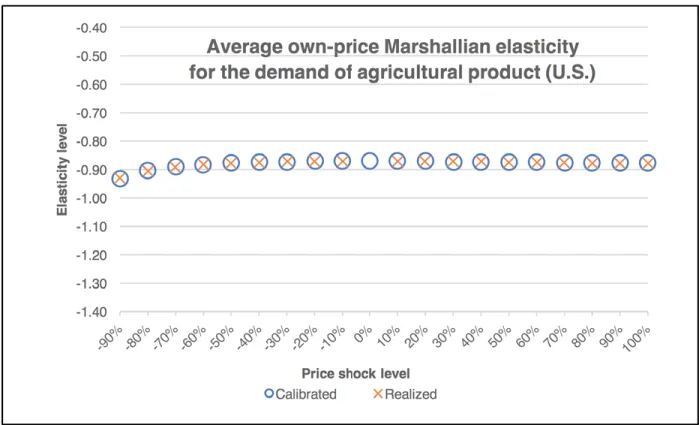
Let us parameterize the revised CGE model of GTAP-8inGAMS, based on calibrated parameters in Table 3. In the model, the aggregated primary factor along with the choice of the numeraire, which is the price for the aggregated primary factor, facilitate the identification of income effect. Now, to verify whether the CDE system is correctly implemented, the study will test if the outputs of the CGE model are consistent to the underlying cal-ibrated elasticities under given price or income shocks. For example, with the shock on the price of agricultural product in the U.S., the first exercise changes the cost of final consumption for agricultural product in the U.S. ex-Table 3. Performance of the cDe calibration under the setting “2r4s1f”
θ_i α_i e_i σ^( ct )_( ii) σ^( cc )_( ii) η_i^ t η _ i^ c Region: USA agri 0.04909 0.85705 2.00000 -0.67034 -0.82165 0.81292 0.99981 man 0.18381 0.99999 0.00000 -0.82044 -0.81489 0.99514 1.00000 tran 0.20250 0.99999 0.00000 -0.85294 -0.79607 1.01152 1.00000 serv 0.56460 0.99999 3.37350 -0.85273 -0.43143 1.01372 1.00002 Distance 0.31937 0.04303 Region: ROW agri 0.14694 0.39172 0.18712 -0.39520 -0.40556 0.71822 0.71822 man 0.27510 0.87997 0.18541 -0.62097 -0.63723 1.00104 1.00104 tran 0.25415 0.99999 0.00000 -0.70506 -0.71473 1.05431 1.07113 serv 0.32380 0.99999 1.13413 -0.72614 -0.63656 1.08436 1.07116 Distance 0.05206 0.01133
ogenously to create the considered price shock.6 The goal
is to calculate the uncompensated (Marshallian) average own-price elasticity for the demand of agricultural prod-uct based on the model response, and see if the realized elasticity from the model output is consistent to the cal-ibrated level.
It is worth noting that while the target own-price elasticity for the demand of agricultural product is σ_(ii)^(
ct
)
=- 0.6703, the calibrated own-price demand elas-ticity is σ_(ii)^(
cc
)
=- 0.8217, which again is evidence that the CDE system is not own-price flexible (Table 3). Be-sides, since with a nontrivial price shock imposed on the CGE model, it is more convenient to derive a “realized” uncompensated average demand elasticity based on the model’s output, for comparison purposes, the study will also convert the calibrated own-price demand elastici-ty σ_(ii)^(
cc
)
, which is a compensated point elasticity, into an uncompensated average demand elasticity with the same price shock so one can easily compare the realized level to the calibrated one.
The calibrated uncompensated own-price demand elas-ticity, σ_(ii)^(
m
)
=- 0.8707 (a point elasticity), can be derived from σ_(ii)^(
c
)
, η_(i), and θ_(i) based on the Slutsky equation
pre-6 For instance, in the revised CGE model of GTAP8inGAMS, a 10% increase in the price of agricultural product is achieved by multiplying both vdfm(“agri”, c, “usa”) and vifm (“agri”, c, “usa”) by 1.1.
sented in Equation (2). Let us consider the quantity in-dex q̃_(i)=q_(i)/θ_(i) with the benchmark level q̃_(0i)=1 since
q_(oi)=θ_(i) (see Step 3 in Section 3.1). Because the
percent-age change in q̃_(i) is equivalent to the percentage change
in q_(i), q̃_(i) can replace q_(i) in deriving the average
uncom-pensated (Marshallian) demand elasticity —with both price and quantity indices normalized to unity, σ_(ii)^(
ma
)
can be expressed as:
(14)
p_(i) is the after- shock price level
When various price shocks of agricultural product are in place, the values for σ_(ii)^(
ma
)
(the calibrated average Marshal-lian demand elasticity) and the realized average elastici-ty levels σ_(ii)^(
mar
)
(derived from the model output) are both presented in Figure 1. Note that with the exogenous price shocks in agricultural product, in the new equilibrium, one may also observe changes in prices of other com-modities relative to their pre-shock levels, and this will in turn affect the equilibrium food consumption level due to the existence of cross-price elasticities of food demand. The exogenous price shock may also induce an income effect as reflected by the change in total (final) expendi-ture level. Therefore, to calculate σ_(ii)^(
mar
), the consumption
index q̃_(i) is adjusted such that it is net of the cross-price
and income effects. The result in Figure 1 shows that, as expected, the larger the price shock, the more the average elasticity deviates from the point elasticity σ_(ii)^(
m
)
, which is the calibrated level without any price shock in the figure. Figure 1 also verifies that the uncompensated average de-mand elasticity σ_(ii)^(
mar
)
calculated from the model output replicates its calibrated counterpart σ_(ii)^(
ma
)
.
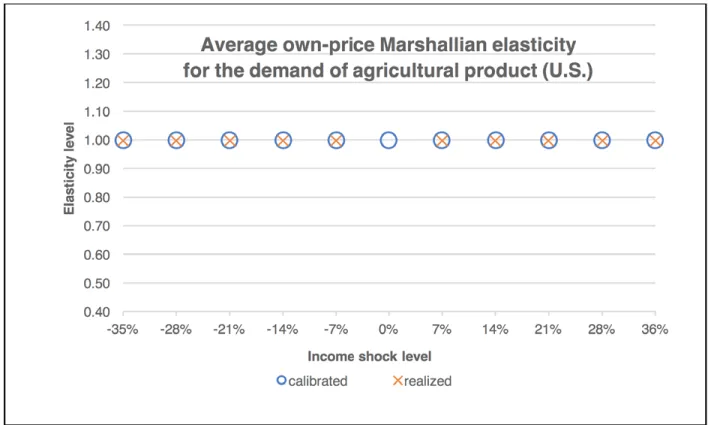
In the following exercise, the study examines the model response under various income shocks in the U.S. The shocks are created by changing the quantity of the ag-gregated primary factor of the U.S., which is just the real GDP level of the U.S. Since GDP is not only spent on private consumption, to calculate the income elasticities of various commodities based on the model response, instead of using the percentage change in GDP as the de-nominator of the elasticity, one needs to use the percent-age change in the portion of income dedicated to private consumption, or equivalently, the percentage change in total expenditure on private consumption. Following the same logic as Equation (14), the average income demand elasticity can be written as:
(15)
c is the after- shock income level
Under various levels of income shock, Equation (15) is used to convert the calibrated point elasticity into the calibrated average elasticity, which serves as the bench-mark for the comparison between the realized average elasticity from model outputs and the calibrated level the model is given. Finally, as the previous example, the new equilibrium with an income shock,
will generally accompany changes in price levels of var-ious commodities. This means that the resulting con-sumption levels will be contaminated by changes in pric-es, although these changes are usually small. The study accounts for this price effect and removes it from the con-sumption levels, and then for each commodity, uses the percentage change of the adjusted consumption level as the numerator of the income elasticity. Figure 2 demon-strates that for the final consumption of agricultural product, the realized average income demand elasticity levels, as expected, replicate their calibrated counter-parts. The two exercises presented here can be extended to other sectors and regions. For instance, with this 2-re-gion and 4-sector setting, most of the calibrated income demand elasticities are close to one. The only exception is the income demand elasticity for the agricultural prod-uct in the rest of the world, η_(i)^(
c
)=0.7182 (Table 3). For
this elasticity, the calibrated and the realized numbers are matched as well (Figure 3).
4. Conclusion
This is the first paper to explore the circumstances under which the calibrated own-price and income elasticities of demand in a CDE demand system can be matched more accurately to their target levels. It finds that while the system is neither own-price nor income flexible, the elasticity match improves with lower sectorial expendi-ture shares (or a higher sectorial resolution), lower target own-price demand elasticities, and higher target income demand elasticities. In any case, to understand the extent to which the elasticity targets are correctly represented in a CGE model, it is crucial to check whether the tar-get elasticities are valid (i.e., compatible to a NSD Slutsky matrix), and disclose how well the calibrated elasticities match their target counterparts. Without having these inspections, when the calibrated elasticities deviate from target levels, it will not be possible to determine if that is due to targeting elasticity levels that are invalid, or if the inflexibility of the demand system is indeed the cause of the mismatch.
In addition, using GTAP8inGAMS, the study also incor-porates the CDE demand system into a global CGE model written in MPSGE, which has not been presented before.
Furthermore, price and income shocks are imposed on this revised GTAP8inGAMS, and the model responses successfully replicate the calibrated elasticities of the CDE demand system. Future studies may examine if other CGE applications with the CDE demand can produce results consistent to the calibrated elasticities, or they may inves-tigate the flexibility and calibration performance of other demand systems. These issues are rarely studied, but are essential for reasons discussed in this research.
Acknowledgments
The author gratefully acknowledges the financial support for this work provided by the MIT Joint Program on the Science and Policy of Global Change through a consortium of industrial and foundation sponsors and Federal awards, including the U.S. Department of Energy, Office of Science under DEFG02-94ER61937 and the U.S. Environmental Protection Agency under XA83600001-1. For a complete list of sponsors and the U.S. government funding sources, please visit http://globalchange.mit.edu/sponsors/all. The discussions with Tom Rutherford about the regularity and flexibility of a demand system are instrumental to this study. Also, the author is thankful for comments from Tom Hertel, Ching-Cheng Chang, three anonymous reviewers, participants of the MIT EPPA meeting, the 18th GTAP
Conference in Melbourne, Australia, and the 2015 Taiwan Economic Association annual conference. Edits and suggestions from Jamie Bartholomay are highly appreciated. All remaining errors are my own. Figure 3. Average income elasticity for the agricultural product demand in the rest of world
5. References
ABARE (Australian Bureau of Agricultural and Resource Economics), 1996: The MEGABARE Model. Interim Documentation, Canberra. ABARE and DFAT (Department of Foreign Affairs and Trade), 1995:
Global Climate Change: Economic Dimensions of a Cooperative International Policy Response Beyond 2000. Canberra.
Allen, G.D. and J.R. Hicks, 1934: A Reconsideration of the Theory of Value, Part II, Economica 1, 196–219.
Annabi, N., J. Cockburn, and B. Decaluwé, 2006: Functional Forms and Parametrization of CGE Models, MPIA Working Paper, PEP-MPIA, Cahiers de recherche MPIA (http://www.un.org/en/ development/desa/policy/mdg_workshops/entebbe_training_ mdgs/ntbtraining/annabi_cockburn_decaluwe2006.pdf). Chern, W.S., K. Ishibashi, K. Taniguchi, and Y. Tokoyama, 2003:
Analysis of the food consumption of Japanese households, FAO Economic and Social Development Paper No. 152, Food and Agriculture Organization of the United Nations (ftp://ftp.fao.org/ docrep/fao/005/y4475E/y4475E00.pdf).
Elsenburg, 2003: Functional forms used in CGE models: Modelling production and commodity flows. The Provincial Decision Making Enabling Project Background Paper, 2003: 5, South Africa (http://www.elsenburg.com/provide/documents/ BP2003_5%20Functional%20forms.pdf).
Ferris, M.C. and J.S. Pang, 1997: Engineering & Economic Applications of Complementarity Problems. SIAM Review 39(4): 669–713. Geary, R.C., 1950: A Note on “A Constant-Utility Index of the Cost of
Living”. Review of Economic Studies 18, 65–66.
Global Trade Analysis Project (GTAP), 2015: GTAP Data Bases: Detailed Sectoral List. Center for Global Trade Analysis, Department of Agricultural Economics, Purdue University, West Lafayette, Indiana (https://www.gtap.agecon.purdue.edu/ databases/contribute/detailedsector.asp).
Hanoch, G., 1975: Production and Demand Models with Direct or Indirect Implicit Additivity, Econometrica, 43(3): 395–419. Haque, M.O., 2005: Income Elasticity and Economic Development:
Methods and Applications. 277 p., Springer.
Hertel, T.W., R. McDougall, B. Narayanan and A. Aguiar, 2014: GTAP 8 Data Base Documentation - Chapter 14 Behavioral Parameters. Center for Global Trade Analysis, Department of Agricultural Economics, Purdue University, West Lafayette, Indiana (https://www.gtap.agecon.purdue.edu/resources/res_ display.asp?RecordID=4551).
Hertel, T.W., 2012: Global Applied General Equilibrium Analysis Using the Global Trade Analysis Project Framework, Handbook of Computable General Equilibrium Modeling, Chapter 12, 815–876.
Hertel, T.W. and M.E. Tsigas, 1997: Structure of GTAP, Global Trade Analysis: Modeling and Applications Chapter 2, 13–73. New York, Cambridge University Press.
Hertel, T.W., P.V. Preckel, M.E. Tsigas, E.B. Peterson, and Y. Surry, 1991: Implicit Additivity as a Strategy for Restricting the Parameter Space in Computable General Equilibrium Models, Economic and Financial Computing 1, 265–289.
Huff, K., K. Hanslow, T.W. Hertel, and M.E. Tsigas, 1997: GTAP Behavior Parameters, Global Trade Analysis: Modeling and Applications, Chapter 4, 124–148. New York, Cambridge University Press.
Konovalchuk, V., 2006: A Computable General Equilibrium Analysis of the Economic Effects of the Chernobyl Nuclear Disaster, The Graduate School College of Agricultural Sciences, Pennsylvania State University, 175 p.
Liu, J., Y. Surry, B. Dimaranan, and T. Hertel, 1998: CDE Calibration, GTAP 4 Data Base Documentation, Chapter 21, Center for Global Trade Analysis, Purdue University (https:// www.gtap.agecon.purdue.edu/resources/download/291.pdf). Markusen, J., 2013: General-Equilibrium Modeling using GAMS and MPS/GE: Some Basics. University of Colorado, Boulder (http://spot.colorado.edu/~markusen/teaching_files/applied_general_ equilibrium/GAMS/ch1.pdf).
Mas-Colell, A., M.D. Whinston, and J.R. Green, 1995: Microeconomic Theory, Oxford University Press.
Mathiesen, L., 1985: Computation of Economic Equilibra by a Sequence of Linear Complementarity Problems. Mathematical Programming Study 23: 144–162.
Perroni, C., and T. Rutherford, 1995: Regular Flexibility of Nested CES Functions. European Economic Review 39, 335–343.
Perroni, C., and T. Rutherford, 1998: A Comparison of the Performance of Flexible Functional Forms for Use in Applied General
Equilibrium Modelling. Computational Economics 11, 245–263. Reimer, J. and T. Hertel, 2004: Estimation of International Demand Behaviour for Use with Input-Output Based Data. Economic Systems Research 16(4), 347–366.
Rimmer, M. and A. Powell, 1996: An implicitly additive demand system. Applied Economics 28, 1613–1622.
Rutherford, T. 1999: Applied General Equilibrium Modeling with MPSGE as a GAMS Subsystem: An Overview of the Modeling Framework and Syntax. Computational Economics 14: 1–46. Rutherford, T. 1995: Extension of GAMS for Complementarity
Problems Arising in Applied Economic Analysis. Journal of Economic Dynamics and Control 19: 1299–1324.
Rutherford, T. 2012: The GTAP8 Buildstream. Wisconsin Institute for Discovery, Agricultural and Applied Economics Department, University of Wisconsin, Madison.Sancho, F., 2009: Calibration of CES functions for ‘real-world’ Multisectoral Modeling. Economic Systems Research 21(1), 45–58.
Stone, R., 1954: Linear Expenditure Systems and Demand Analysis: An Application to the Pattern of British Demand. Economic Journal 64, 511–527.
Uzawa, H., 1962: Production Functions with Constant Elasticities of Substitution, Review of Economic Studies 30, 291–299. van der Mensbrugghe, D., 2008: Environmental Impact and Sustainability Applied General Equilibrium (ENVISAGE) Model. Development Prospects Group, The World Bank. (http://siteresources.worldbank.org/INTPROSPECTS/ Resources/334934-1193838209522/Envisage7b.pdf)
Woltjer, G.B. and M.H. Kuiper, 2014: The MAGNET Model: Module description. Wageningen, LEI Wageningen UR (University & Research centre), LEI Report 14-057. 146 p. (http://www. magnet-model.org/MagnetModuleDescription.pdf)
Zeitsch, J., R. McDougall, P. Jomini, A. Welsh, J. Hambley, S. Brown, and J. Kelly, 1991. SALTER: A General Equilibrium Model of the World Economy. SALTER Working Paper N. 4. Canberra, Australia: Industry Commission.
Zhou, Z., W. Tian, J. Wang, H. Liu, and L. Cao, 2012: Food Consumption Trends in China. Report submitted to the Australian Government Department of Agriculture, Fisheries and Forestry (http://www.agriculture.gov.au/ SiteCollectionDocuments/agriculture-food/food/publications/ food-consumption-trends-in-china/food-consumption-tre nds-in-china-v2.pdf).
Appendix A: The CDE Calibration Program
77 This GAMS program implements the three-step procedure for calibrating the CDE system. To run it, one needs: 1) the GTAP 8 data in the gdx format (created by GTAP8inGAMS) with desired resolutions for regions, sectors, and primary factors; 2) the subroutine “gtap8data.gms,” which is also included in GTAP8inGAMS, that reads data needed in the calibration program; 3) to type “gams cdecalib” under the DOS command prompt—this will use the default database “2r4s1f.gdx”. The environment variable “ds” can be used to overwrite the default database setting.
Appendix B: The CGE Model with CDE Demand for GTAP8inGAMS
88 To run this MPSGE program “mrtmge_cde.gms,” one needs to 1) place it inside the subdirectory “model” of GTAP8inGAMS; 2) set either price shock or income shock within the loop; 3) set the output file name that distinguishes price shock from income shock; and 4) type, for exam-ple, “gams mrtmge_cde --start=0.1 --end=20 --step=0.1” under the DOS command prompt. With the default setting, this will produce 20 different price shocks for the agricultural product—the first shock will be created by multiplying both vdfm(“agri”,c,”usa”) and vifm(“agri”,c,”usa”) by 0.1, and for each following shock, the multiplicand increases by 0.1 compared to that in the previous shock.
Appendix D: Calibration Details of the CDE System
θ α ϵ_(target) ϵ_(calibrated) e η_(target) η_(calibrated) 1r3s2f s01 0.11779 0.69132 -0.42935 -0.64196 1.00000 0.72997 0.99993 s02 0.24791 0.99999 -0.66503 -0.74307 0.00000 0.99974 1.00000 s03 0.63430 0.99999 -0.76584 -0.34264 1.39128 1.05025 1.00001 1r4s2f s01 0.11779 0.46593 -0.42935 -0.46570 1.69852 0.72997 0.84424 s02 0.24791 0.97108 -0.66503 -0.72013 0.00000 0.99974 1.00000 s03 0.23876 0.99999 -0.74242 -0.74450 0.00000 1.04350 1.02891 s04 0.99999 -0.77997 -0.57674 6.05841 1.05432 1.02894 1r5s2f s01 0.03432 0.25519 -0.20559 -0.26903 0.34455 0.55041 0.55041 s02 0.11603 0.64030 -0.52076 -0.59769 0.37632 0.81865 0.81865 s03 0.10413 0.81460 -0.66544 -0.74006 0.81022 1.00727 1.00727 s04 0.28309 0.99999 -0.75108 -0.69238 1.03185 1.05134 1.04791 s05 0.46242 0.99999 -0.76079 -0.49752 1.30986 1.04581 1.04791 1r8s2f s01 0.03352 0.21620 -0.19417 -0.23118 1.77964 0.53872 0.53872 s02 0.02279 0.52803 -0.48782 -0.52400 2.53677 0.81197 0.81197 s03 0.09404 0.60345 -0.53011 -0.57264 2.17642 0.82213 0.82213 s04 0.09783 0.77401 -0.66566 -0.70859 4.08792 1.00456 1.00456 s05 0.04364 0.79038 -0.72192 -0.75976 4.69953 1.03290 1.03289 s06 0.07051 0.78613 -0.69707 -0.73727 4.80226 1.03684 1.03683 s07 0.24214 0.99999 -0.74111 -0.72864 0.99992 1.04339 1.05016 s08 0.39553 0.99999 -0.77997 -0.55674 9.13649 1.05432 1.05018 1r16s2f s01 0.02937 0.15660 -0.16693 -0.17214 0.28241 0.48744 0.48744 s02 0.00415 0.39182 -0.38712 -0.39206 0.63398 0.90206 0.90206 s03 0.00092 0.67054 -0.66517 -0.67008 0.82138 1.04085 1.04085 s04 0.02187 0.48840 -0.48033 -0.48546 0.43837 0.80230 0.80230 s05 0.01917 0.42077 -0.41568 -0.42078 0.38537 0.73339 0.73339 s06 0.07487 0.59054 -0.55941 -0.56517 0.42817 0.84486 0.84486 s07 0.03095 0.65777 -0.63789 -0.64312 0.63971 0.96517 0.96517 s08 0.06687 0.72478 -0.67851 -0.68417 0.76744 1.02279 1.02279 s09 0.00330 0.65472 -0.64824 -0.65318 0.84878 1.05236 1.05236 s10 0.04035 0.76068 -0.72795 -0.73328 0.78856 1.03131 1.03131 s11 0.04451 0.74928 -0.71468 -0.72006 0.80920 1.03715 1.03715 s12 0.02600 0.68584 -0.66691 -0.67208 0.80951 1.03631 1.03631 s13 0.20777 0.99999 -0.75135 -0.75945 0.89823 1.05178 1.04092 s14 0.03437 0.70394 -0.67923 -0.68450 0.68774 0.99270 0.99270 s15 0.13072 0.93955 -0.79738 -0.80402 1.60728 1.09873 1.09873 s16 0.26481 0.99999 -0.77138 -0.69341 0.67100 1.03240 1.04092
θ α ϵ_(target) ϵ_(calibrated) e η_(target) η_(calibrated) 1r29s2f s01 0.00143 0.09267 -0.09357 -0.09357 0.42740 0.33991 0.33991 s02 0.01600 0.10522 -0.11479 -0.11479 0.40249 0.33825 0.33825 s03 0.00069 0.09841 -0.09883 -0.09883 0.62831 0.43748 0.43748 s04 0.00290 0.13154 -0.13312 -0.13312 0.47413 0.39110 0.39110 s05 0.00520 0.30895 -0.30995 -0.30995 1.33837 0.83221 0.83221 s06 0.00315 0.27425 -0.27506 -0.27506 1.39632 0.84299 0.84299 s07 0.00398 0.38575 -0.38590 -0.38590 1.46331 0.89563 0.89563 s08 0.00017 0.41754 -0.41753 -0.41753 1.97351 1.05623 1.05623 s09 0.00092 0.66584 -0.66536 -0.66536 1.90474 1.04089 1.04089 s10 0.01817 0.51877 -0.51461 -0.51461 1.00120 0.81432 0.81432 s11 0.01690 0.46672 -0.46461 -0.46461 1.05382 0.80348 0.80348 s12 0.00597 0.21068 -0.21299 -0.21299 0.69651 0.54116 0.54116 s13 0.06527 0.57659 -0.55410 -0.55410 0.93506 0.82800 0.82800 s14 0.02982 0.64004 -0.62598 -0.62598 1.45830 0.95776 0.95776 s15 0.01073 0.63809 -0.63307 -0.63307 1.58403 0.98065 0.98065 s16 0.03895 0.69602 -0.67330 -0.67330 1.68759 1.00760 1.00760 s17 0.03068 0.70071 -0.68252 -0.68252 1.92233 1.04433 1.04433 s18 0.00054 0.64150 -0.64124 -0.64124 2.09503 1.07543 1.07543 s19 0.03579 0.76118 -0.73564 -0.73564 1.84873 1.03603 1.03603 s20 0.01658 0.69629 -0.68660 -0.68660 1.81666 1.02778 1.02778 s21 0.03249 0.74450 -0.72240 -0.72240 1.85417 1.03591 1.03591 s22 0.02171 0.67285 -0.66119 -0.66119 1.88490 1.03770 1.03770 s23 0.00765 0.67912 -0.67491 -0.67491 1.85026 1.03219 1.03219 s24 0.20439 0.99418 -0.75305 -0.75305 3.31501 1.05204 1.05204 s25 0.00855 0.63947 -0.63545 -0.63545 1.67133 0.99708 0.99708 s26 0.06077 0.80464 -0.75598 -0.75598 2.10861 1.06429 1.06429 s27 0.09577 0.88842 -0.79570 -0.79570 2.70728 1.09161 1.09161 s28 0.17177 0.96520 -0.77251 -0.77251 1.01877 1.03136 1.03136 s29 0.09304 0.85273 -0.76929 -0.76929 1.76577 1.03432 1.03432 s01 0.00681 0.65433 -0.65067 -0.65067 0.30974 0.99476 0.99476 s02 0.02640 0.56879 -0.55911 -0.55911 0.18143 0.83196 0.83196 s03 0.00017 0.09099 -0.09111 -0.09109 0.09240 0.36960 0.36960 s04 0.02582 0.71052 -0.69373 -0.69373 0.29289 0.99124 0.99124 s05 0.00775 0.52036 -0.51827 -0.51827 0.18304 0.80914 0.80914 s06 0.00337 0.65002 -0.64823 -0.64823 0.35438 1.03589 1.03589 s07 0.00017 0.41702 -0.41692 -0.41701 0.37516 1.05659 1.05659 s08 0.02792 0.70352 -0.68575 -0.68575 0.36117 1.04398 1.04398 s09 0.00078 0.27528 -0.27545 -0.27545 0.28216 0.87675 0.87675 s10 0.09304 0.85704 -0.76927 -0.76927 0.32303 1.03432 1.03432 s11 0.01203 0.70142 -0.69382 -0.69382 0.35690 1.04050 1.04050 s12 0.01903 0.66669 -0.65599 -0.65599 0.35670 1.03880 1.03880 s13 0.00301 0.67887 -0.67710 -0.67711 0.36430 1.04588 1.04588
θ α ϵ_(target) ϵ_(calibrated) e η_(target) η_(calibrated) s14 0.00105 0.48534 -0.48513 -0.48513 0.37597 1.05735 1.05735 s15 0.00293 0.35032 -0.35053 -0.35052 0.24937 0.83797 0.83797 s16 0.00081 0.68067 -0.68020 -0.68020 0.35220 1.03557 1.03557 s17 0.00273 0.69484 -0.69315 -0.69315 0.34460 1.03015 1.03015 s18 0.00152 0.11160 -0.11243 -0.11243 0.11440 0.43746 0.43746 s19 0.00026 0.60859 -0.60854 -0.60847 0.40425 1.08610 1.08610 s20 0.02590 0.77890 -0.75851 -0.75851 0.31258 1.01763 1.01763 s21 0.00739 0.60771 -0.60442 -0.60442 0.27705 0.95247 0.95247 s22 0.00334 0.69847 -0.69638 -0.69638 0.36011 1.04296 1.04296 s23 0.01320 0.51068 -0.50737 -0.50737 0.19535 0.82036 0.82036 s24 0.03278 0.76596 -0.74100 -0.74100 0.34384 1.03512 1.03512 s25 0.00028 0.67218 -0.67193 -0.67202 0.38674 1.06543 1.06543 s26 0.00276 0.65106 -0.64960 -0.64959 0.36712 1.04786 1.04786 s27 0.00442 0.31545 -0.31607 -0.31607 0.24823 0.82431 0.82431 s28 0.06985 0.87837 -0.80949 -0.80949 0.57418 1.11904 1.11904 s29 0.00239 0.06962 -0.07113 -0.07113 0.05907 0.27043 0.27043 s30 0.03887 0.56463 -0.55069 -0.55069 0.17756 0.82531 0.82531 s31 0.03495 0.83329 -0.80198 -0.80198 0.51806 1.11825 1.11825 s32 0.00000 0.54565 -0.54574 -0.54565 0.34258 1.01626 1.01626 s33 0.01632 0.73209 -0.72077 -0.72077 0.34887 1.03608 1.03608 s34 0.01617 0.73536 -0.72405 -0.72405 0.34810 1.03574 1.03574 s35 0.00012 0.56284 -0.56280 -0.56280 0.39380 1.07767 1.07767 s36 0.01042 0.51457 -0.51188 -0.51188 0.19225 0.81818 0.81818 s37 0.00052 0.10104 -0.10135 -0.10134 0.12667 0.45970 0.45970 s38 0.10513 0.88557 -0.78040 -0.78040 0.29993 1.03107 1.03107 s39 0.00456 0.67014 -0.66755 -0.66755 0.30611 0.99424 0.99424 s40 0.03252 0.62968 -0.61379 -0.61379 0.31758 0.99835 0.99835 s41 0.02743 0.66120 -0.64607 -0.64607 0.31057 0.99669 0.99669 s42 0.00350 0.10424 -0.10620 -0.10620 0.09453 0.38467 0.38467 s43 0.00029 0.12906 -0.12919 -0.12921 0.16415 0.56568 0.56568 s44 0.00052 0.41959 -0.41952 -0.41956 0.30542 0.94812 0.94812 s45 0.01153 0.74657 -0.73824 -0.73824 0.34381 1.03358 1.03358 s46 0.00296 0.27504 -0.27569 -0.27569 0.26158 0.83670 0.83670 s47 0.06663 0.81767 -0.76006 -0.76006 0.32874 1.03182 1.03182 s48 0.00248 0.36364 -0.36375 -0.36375 0.20224 0.76202 0.76202 s49 0.00960 0.59960 -0.59548 -0.59548 0.28551 0.95945 0.95945 s50 0.17186 0.98578 -0.77940 -0.77940 0.60041 1.06220 1.06220 s51 0.01448 0.10698 -0.11504 -0.11504 0.06992 0.32782 0.32782 s52 0.00370 0.31151 -0.31206 -0.31206 0.20503 0.74329 0.74329 s53 0.02022 0.65120 -0.64045 -0.64045 0.26986 0.95695 0.95695 s54 0.00115 0.08393 -0.08462 -0.08462 0.05940 0.28326 0.28326 s55 0.00019 0.26531 -0.26536 -0.26536 0.31734 0.94356 0.94356 s56 0.00174 0.57650 -0.57583 -0.57583 0.33148 1.00619 1.00619 s57 0.00428 0.69859 -0.69591 -0.69591 0.34315 1.02927 1.02927