Key performance indicators to enhance water distribution network resilience in three-stages

HAL Id: hal-02264086

https://hal.archives-ouvertes.fr/hal-02264086

Submitted on 6 Aug 2019

HAL is a multi-disciplinary open access

archive for the deposit and dissemination of sci-entific research documents, whether they are pub-lished or not. The documents may come from teaching and research institutions in France or abroad, or from public or private research centers.

L’archive ouverte pluridisciplinaire HAL, est destinée au dépôt et à la diffusion de documents scientifiques de niveau recherche, publiés ou non, émanant des établissements d’enseignement et de recherche français ou étrangers, des laboratoires publics ou privés.

Key performance indicators to enhance water

distribution network resilience in three-stages

David Ayala Cabrera, Olivier Piller, Jochen Deuerlein, Manuel Herrera

To cite this version:

David Ayala Cabrera, Olivier Piller, Jochen Deuerlein, Manuel Herrera. Key performance indicators to enhance water distribution network resilience in three-stages. Water Utility Journal, 2018, 19, pp.79-90. �hal-02264086�

Key performance indicators to enhance water distribution network

resilience in three-stages

D. Ayala-Cabrera1*, O. Piller1, J. Deuerlein2 and M. Herrera3 1 _{Irstea, UR ETBX, Dept. of Water, F-33612 Cestas, France}

2 _{3S Consult GmbH, D 76137 Karlsruhe, Germany}

3 _{EDEn-ACE Dept., University of Bath, Claverton Down, BA2 7AY Bath, UK} * _{e-mail: david.ayala@irstea.fr}

Abstract: Water distribution networks (WDNs) are critical infrastructures that should face multiple and continuous changes and adverse operative conditions (due to abnormal events) that alter their normal service provision. The main objective of a WDN is to deliver the required amount of water to the customer under a certain threshold of the desired pressure and quality. Therefore, ensuring resilience and safety of WDSs are big concerns for water utilities. Several resilience key performance indicators have been suggested to quantify and assessing WDN resilience. Regarding the objectives of resilience, water utility managers require modelling tools to be able to predict how the WDN will perform during disruptive events and understand how the system can better absorb them. Tools such as: demand-driven modelling (DDM) for sufficient pressure conditions, and pressure-driven modelling (PDM) for insufficient pressure conditions, aid to simulate WDNs performance under adverse operative conditions. This work attempts to evaluate the network resilience. The proposed approach is based on an event-driven methodology and there is considered the time when the event occurs, when it evolves, and the sequence of the events. It should be carefully selected the type of the approach (PDM or DDM) used for the hydraulic model, as well as the system performance state and the uses of resilience power-based indicators. The results are promising in order to provide to water managers with a great depth of information and support better preparedness for WDNs.

Key words: resilience; resilience key performance indicators; water distribution networks; critical infrastructures

1. INTRODUCTION

Water distribution networks (WDNs) provide an essential service on life and wellbeing for cities inhabitants at safety level and acceptable costs (Large et al., 2015). The main objective of a WDN is to deliver the required amount of water to customers under a certain threshold of a desired pressure and quality (Jung, 2013). WDNs are critical infrastructures that should face multiple changes and to eventually cope with abnormal events that alter their service. Disruptive events produce potential impact at the networks such as: pipe breaks, other infrastructure damage/failure as power outage – critical infrastructure interdependencies, service outages, loss of access to facilities, loss of head pressure, changes in water quality, environmental impacts, financial impacts and social impacts, among others. In practice, water asset management is a complex multi-criteria problem since managers must prevent or minimize the potential damage (Large et al., 2015), as result of the potential disruptive events. Nowadays, water utility managers require modelling tools to predict how the WDN performs during disruptive events and to understand how the system can best absorb, successfully adapt, and recover from them. Simulation and analysis tools aid WDN managers to explore how their networks respond to unexpected events. In this context, demand-driven modelling (DDM) for normal operating conditions and pressure-driven modelling (PDM) for failure conditions, aid to simulate WDN performance under failure event conditions.

Any potential hazard is mainly classified in natural disasters (e.g. earthquakes, floods, etc.), intentional attacks (terrorist attacks), and materials release. The risk environment that affects critical infrastructure (such as WDNs) is complex and uncertain in relation to threats, vulnerabilities, and consequences. The increasing size of the urban infrastructure along with its associated

communication technologies to manage critical infrastructure operations create new cyber vulnerabilities to handle by utility managers at any big city nowadays (NIPP, 2013).

Water network security refers to have a water supply under safety conditions for consumers. To guarantee this security is necessary to assess all type of potential vulnerabilities. In addition, a WDN need to provide the required quantity of water for sensitive customers, such as hospitals, under any circumstance (NIPP, 2013). Risk costs regarding WDNs users’ health should be considered in the water management decision making in terms of customer incomes or medical treatments costs. The consequences are thereby much greater than the cost of replacing deficient pipes (Ilaya-Ayza et al., 2016). In this context, what is resilience? On the one hand, we have the infrastructural resilience that is defined as the ability to reduce the magnitude, impact, or duration of a disruption (NIAC, 2009). On the other side, resilience refers to the strength of the network and its behaviour under anomalous events. Resilience may also be perceived as a more general concept that relies on three system capabilities: 1) absorptive, 2) adaptive, and 3) restorative (Ouyang et al., 2012). Resilience can be characterized by four properties / attributes: 1) robustness, 2) redundancy, 3) resourcefulness and 4) rapidity (Tierney and Bruneau, 2007) A multi-disciplinary resilience approach should comprises technical, organizational, social and economic aspects. The more classical resilience concept, provided by Bruneau et al. (2003), suffers a number of lacks in terms of the notion of preparedness, covering for instance emergency plans, early detection, etc. (Francis and Bekera, 2014). Resilience of a water network refers to design maintenance, and operations of water supply infrastructure that limit the effects of disruptions and enable rapid return to normal delivery of safe water to customers (Ayala-Cabrera et al., 2017a). In the context of critical infrastructures, resilience can be developed by focusing on the different stages of the performance following a disturbance (also called resilience curve), and devising strategies and improvements, which strengthens the system response (IRGC, 2016). Therefore, assessing and enhancing resilience in water infrastructures is a crucial step towards a more sustainable urban water management. As a prelude to an enhancing resilience, a detailed understanding is required of the inherent resilience underlying system (Diao et al., 2016).

This work proposes a structured evaluation of the network performance by means of resilience key performance indicators (rKPIs). The proposed approach is based on an event-driven approach and supported by the conceptual definition proposed by the Franco-German ResiWater Project (ResiWater, 2017). In ResiWater Project the notion of resilience attempts to develop tools to prepare water utilities for crisis by enhancing water network resilience. This improves the approach proposed by Francis and Bekera, (2014) by inclusion of the preparedness. For the sake of simplicity, this paper works on water quantity issues using a hypothetical benchmark network. This allows to derive essential preliminary network resilience results, to use resilience indicators under two different modelling approaches (DDM and PDM), and to quantify the three resilience stages of the network resilience (based on the three-capabilities of the system). Aspects such as time when the abnormal event occurs and its developed, the sequence of the events, the differences in the resilience and the performance states results as consequence of the hydraulic model used, and the uses of the classical and new resilience power-based indicators are contemplated as well. Ultimately, this work seeks to provide engineers, modellers, and managers with structured tools, which allow a comprehensive analysis of crisis management case studies with the aim of enhancing the WDN resilience. It is usual to have limited resources in supply. Then, recovery phases have a crucial role in resilience enhancing, while under sufficient availability of resources, deploying redundancy, making critical components stronger and ensuring a rapid recovery are all effective responses of the system (Ouyang et al., 2012).

The remainder of this paper is organised as follows. Section 2 introduces a conceptual definition of the proposed approach, the brief description about topological characteristics of the networks, the approaches used for hydraulic models, and resilience-related metrics. This section also introduces the proposed methodology to evaluate the system resilience in a suitable framework based on three resilience stages. One illustrative case study related to benchmarking network is given in Section 3

to showcase the applicability of the proposed approach. Finally, a conclusions section closes the document.

2. MATERIAL AND METHODS

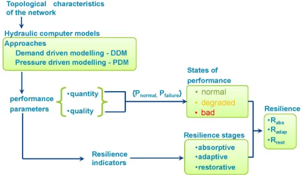
The concept of resilience in the domain of WDNs requires the development of a generic framework that allows knowing the response of the system to different disruptive events. Therefore, there have been developed tools to provide representative information of the system. There are also proposed measures which enable utility managers to adequately quantify the effects of these undesirable events. This section proposes a framework applicable to WDN for assessing resilience to assess the theoretical resilience is presented in Figure 1. The steps involved in this approach are presented in detail below.

Figure 1. Proposed framework to assess theoretical resilience.

2.1 Brief introduction of the three-stages of resilience analysis

As we discussed in the introduction, the ultimate goal of resilience assessment is to preserve the continuity of a normal system function. Normal system performance function is defined according to the fundamental objectives obtained in a previous system identification. The proposed resilience paradigm (ResiWater, 2017) might be implemented via the set of the following resilience capacities: absorptive, adaptive, and restorative capacity. The absorptive capacity refers to the capacity of the system to absorb the impact of any system perturbation and to minimize its consequences (with not action from water utility managers). Adaptive capacity is the ability of the system to temporarily adjust undesirable situations by undergoing some changes if absorptive capacity has been exceeded. Restorative capacity refers to the ability of the system to implement long-term solutions so that the system performance reaches a stable or better level than the initial state (prior to adverse operative conditions).

In reference to the performance states and performance thresholds, there are proposed three different states of WDN performance, P : normal, degraded, and bad. The three states for P are determined by two thresholds: P_normal and P_failure corresponding to minimum P level for the network

working in normal operative mode, and P level when the system is considered in failure mode, respectively. The three-stages of the resilience analysis are:

• Absorptive stage. The absorptive stage is measured since the event starts (t_event) and goes until the water utility starts taking appropriate actions, which is denoted as palliative time (t ). Two additional times involve in this stage are: the degradation time (_pall t ) and the _deg failure time (t ). These correspond to the time at which the first consumer is affected by the _fail event at different states of network performance. Thus, if the t is greater than _deg t , the state _pall for absorptive stage corresponds to the normal state.

For quantifying the resilience for this stage (R ), the three values for resilience are proposed _abs

abs

R = {3, 2, 1} that correspond to the three states at t {normal, degraded, bad}. At this pall

point, the internal vulnerability of the system (V ) is a mirror of the absorptive capacity of _sys the system, and may be assessed as V_sys= 4−R_abs.

• Adaptive stage. The adaptive stage begins before the absorptive stage ends and with the anomaly detection. It is characterized by a stabilization time, t , which is the time when all _stab emergency measures are in place for maintaining the system performance. For instance, at

stab

t , the affected pipes are isolated through valve closure. It lasts until no more temporary solutions are required by the system to reach its contract performance. However, t_stab is not the end of the adaptive phase, as the use of an alternative resource or a palliative solution lasts until the recovery solutions are effective. Some examples of these actions are adapting pump operations (for example, turning on other pumps if available), maintaining storage tanks levels at higher levels enabling additional head (Zhuang et al., 2013), adjusting control valve settings, etc. To qualify the degree of severity, the acceptable time (t ) is defined that _acc corresponds to the maximum stipulated time in which the network can be in failure conditions. t is framed by criteria such as health, social, economic, among others. _acc

The quantification of the resilience in this stage (R_adap) will depend on the state of performance at t=min

(

)

adap

R = {2, 1, 1} with the state {normal, degraded, bad}.

• Restorative stage. The restorative stage begins when t ends, and when long-term solutions stab

begin to be implemented (for instance, repairing or replace affected component). Adaptive and restorative stages end when the system performance reaches a stable level of performance equal or better than the initial one in nominal way (P≥P_normal).

Finally, the resilience for restorative stage will be determined whether the system succeeds in finding a new NORMAL state, then Rrest =3 else it is less.

2.2 Selecting suitable indicators

In the previous section we have raised the reference framework for resilience assessment. There are also required metrics to reflect this framework and to allow knowing the water network performance under undesirable events to provide support to the decision-making process (Francis and Bekera, 2014). The selection of the appropriate measure of resilience depends on the characteristic of the system in order to provide a specific service (IRGC, 2016). In this way, for resilience studies it is key to specify what system state is being considered (resilience of what) and what perturbations are of interest (resilience to what) (Carpenter et al., 2001). In this sense, several studies have been proposed in order to quantify the resilience of WDNs (Herrera et al., 2016). Thereby, in the available literature, the most commonly indicators can be split (based on its approach) into five groups: a) Power/Energy (see e.g. Todini, 2000); b) Performance (see e.g.

Bremond and Berthin, 2001), c) Graph theory/Social networks (see e.g. Herrera et al., 2016), d) time (see e.g. Henry and Ramirez-Marquez, 2012), and e) sensitivities (see e.g. Deuerlein et al., 2017).

In the group of indicators based on system power, the most popular is the resilience index by Todini (2000). The index is a ratio of the power arriving to the users, to the maximum power that can be dissipated in the network to meet the consumer demand. It should be mentioned that the term power is the product of outflow and head. That is, the power is the rate at which energy flows or at which energy is delivered per units of time (Ayala-Cabrera et al., 2017b). To obtain a better representation of the network reliability other authors have proposed other definitions for the Todini’s resilience index such as: minimum surplus head and network resilience index by Prasad and Park (2004) and modified resilience index by Jayaram and Srinivasan (2008), among others. Additional modification for this index, which attempts to include different pressure-dependent modelling, is Saldarriaga et al., (2010). Another modification of Todini's resilience index has been proposed by Creaco et al. (2016). The authors attempt to include in the indicator two different pressure-dependent modelling cases (leakage and consumption).

2.3 Model and equations

Water utility managers require modelling tools to be able to predict how WDNs perform during disruptive events. In this way, mathematical system models play an important role in planning, design and operation of civil engineering projects. These models often require large amounts of data for their implementation and it is often the case that the required data are incomplete, unavailable or uncertain (Tanyimboh, 1993). The hydraulic conditions of water networks have generally been evaluated using DDM models as a function of demand under normal operating conditions and additional PDM implementations which have shown better response to approach WDN analysis under operative conditions of failure. The water distribution computations are approached by a pressure driven model (Piller et al., 2017; Elhay et al., 2016), as in case of pipe failures it provides better description of the system conditions than the classical demand driven model formulations (Creaco et al., 2016). The assumption of fixed nodal consumptions (DDM approaches) is therefore valid only under normal conditions when the pressures can be expected to be adequate to satisfy the stipulated demand. If the operation of the system is simulated under pressure-critical conditions (due to some critical events such as mechanical and hydraulic failures or excess of demand), the relationship between pressure and outflow should, therefore, be taken into account (Moosavian and Jaefarzadeh, 2013) whether the simulations are to be realistic.

The operation of water distribution networks can be assessed by using hydraulic computer models, such as Porteau (Piller et al., 2011) and EPANET (Rossman, 2000), among others. On one side, in the application for systems with inadequate capacity or pipe failure, the classical DDM approach is stretched to its limits (Braun et al., 2017). On the other side, a consumption model that doesn’t consider the available pressure is especially damaging in abnormal situations, such as low pressures resulting from hydraulic and mechanical failures. This is the reason why PDMs have been introduced (Piller et al., 2003).

Topological characteristics of the Network. In hydraulic modelling the simplified topological

structure of a WDN is described by a directed graph. This graph represents pipe sections as links and pipe junctions as nodes. The mathematical description of this graph is given by the incidence matrix N

j i

A, (see, Equation 1).

A_{i, j}N ₌

−1, if nodei isterminalpoint of link j 0, if nodei is not connected to link j 1, if nodei is the initialpoint of link j ⎧ ⎨ ⎪ ⎩ ⎪ (1)

DDM. Matrix _AN _{can be partitioned into two submatrices,}

f

A and A; that represent nodes with fixed head (reservoirs or tanks) and nodes with unknown head (demand or junction nodes), respectively. The equations that describe the steady-state of the system by the potential at the nodes (head) and the current links flows (Piller et al., 2003) are given by Equation 2.

Aq+ d = 0; mass balance at every node

Δh r,q

( )

T_h

f = 0; energy balance every link ⎧

⎨ ⎪ ⎩⎪

(2)

where; q and h are vectors of flow rates in the links and the heads at junction nodes, respectively;

d is the vector of water demand; h_f is the head at fixed head nodes; r is the pipe friction coefficient; Δh ,

( )

PDM. In DDM, nodal demands are always satisfied at all nodes, independent of the available

pressure head values at the corresponding demand nodes. In DDM analysis, available flow at node

i, c (available outflow at node _i i) is always equal to the required consumption d (demand at node _i

i); hence, c_i = (Sivakumar and Prasad, 2014). In contrast, in PDM the outflow is determined by d_i

a relationship between the available pressure head and the outflow. This relation, is denoted Pressure –Outflow Relationship (POR). It contemplates three stages of demand satisfaction; full – outflow, partial or degraded –outflow, and zero –outflow.

The PORs are able to show how the system has the ability to regulate itself in terms of the available outflow and reordering the supply head pressure if it is under failure conditions. In this way, it can be supplied a remainder of delivered flow. Wagner et al. (1988) formulation (Equation 3) is the most accepted POR to evaluate networks operation under failure conditions.

c(h)= d × 1 , if hs≤ h h− h_m h_s− h_m ⎛ ⎝⎜ ⎞ ⎠⎟ 0.5 , if hm < h < hs 0 , if h≤ hm ⎧ ⎨ ⎪ ⎪ ⎩ ⎪ ⎪ (3)

where: h is the service (or reference) head necessary to fully satisfy the required demand; _s h is _m

the head below which no water can be supplied. The latter is the minimum head which is usually defined as nodal elevation. The DDM system (Equation 2) and its PDM counterpart can be solved efficiently by a damped Newton method (Elhay et al., 2016). Moreover, the formulae exist for calculating the DDM and PDM sensitivities with respect to the demand parameter (Piller et al., 2017). These local sensitivities bring important information about the influence of the parameter on the hydraulic state: for example, where to place sensors or confidence intervals for the hydraulic predictions.

3. RESULTS AND COMMENTS

3.1 Definition of the network and performance analysis

The following resilience analysis is based on the three stages of resilience (Section 2.1). A hypothetical network, originally proposed by Islam et al. (2011), it is used to test the proposed

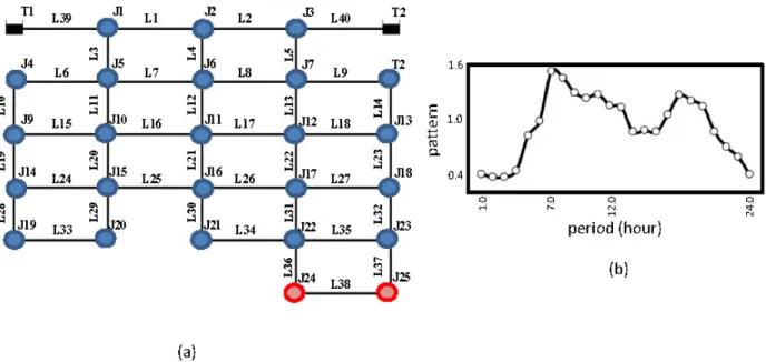
methods. This network has additionally been used for studies of leakage detection (Islam et al., 2011), reliability under uncertainties (Shafiqul et al., 2014) and reliability under cascading failures (Shuang et al., 2014). The network encompasses two reservoirs, twenty-five water demand nodes and forty pipes (Figure 2.a). The water is supplied by gravity from elevated reservoirs (T1 and T2) with total heads of 90 m and 85 m. Pipe length ranges from 100 m to 680 m (total length of all pipes is 19.5 km) and the diameters vary from 200 mm to 700 mm. The basic demand ranges from 33.33 L/s to 133.33 L/s and the demand pattern is defined for 24 hours (Figure 2b). The Hazen-Williams formula is used to calculate the head loss. The selection of this network is due to the size of the network given that it is large enough to show in detail the effects related to the anomalous event. There are sufficient variability of pipe materials and more than one source. The network has been tested under different failure conditions. Further details are presented in (Shuang et al., 2014).

Figure 2. Case study of Islam Network - WDN characteristics. (a) Network layout; and (b) demand curve. A red circle indicates nodes operating under degraded state. Based on Ayala-Cabrera et al. (2017a).

The analysis is developed for all the periods under study and consists in isolating, one by one, every pipe of the system. The process is iterated for each period and it is analysed the performance response at every node. Overall, the analysis is carried out based on the differences to obtained by comparing the failure conditions using for the hydraulic model the DDM and PDM approach.

We have analysed the available pressures at the nodes for each period (Figure 3). The Figure 3 shows how the head pressure at each node is increased under PDM for all tested periods, in opposite to DDM approach. Despite the system regulates itself because of the failure, it is not properly reflected in the DDM approach. Similarly, we can observe (graphically) that in both cases the obtained curve presents a strong correlation with the inverse of the demand patterns (Figure 2.b), in terms of the nodes working under degraded and bad performance state. Figure 3 shows a strong correlation between the obtained values of head pressure when the network is working under normal operative conditions. This global linear behaviour changes when the nodes are working under degraded state of performance (DDM and PDM results are not the same). Figure 3 shows that the maximum effect of failure at any individual system component, namely pipe (isolation), happens at the beginning of the adaptive stage (when some palliative actions are placed from water utility). The issue increases its impact for high demand periods (hours 7 and 8). Figure 3 also shows that, under PDM, the network can self-regulate its pressures by supplying the system with additional energy, enough to meet user’s demands.

Figure 3. Head pressure results – Single pipe isolation (each pipe). Comparison, DDM versus PDM.

3.2 Three-stages of resilience - application through rKPIs

In this study we applied the resilience indicator ( IrT , Equation 4) by Todini (2000), its extension for leakage (IrS, Equation 5) by Saldarriaga et al. (2010), and its generalization (IrC, Equation 6) by Creaco et al. (2016). The interest of the application of these two indicators in this study is mainly because the first indicator operates under DDM, the second under DDM including leakages, and the third works under PDM. All of them let us to quantify the resilience in terms of the available power of the system.

s f f s h d q A h h d h d IrT _{T T} T T − − = (4) s leak f f s leak leak h c d q A h h c d h c d IrS _{T T} T T ) ( ) ( ) ( + − + − + = (5) IrC= max c T_{h− d}T_h s, 0 ⎡⎣ ⎤⎦ hf T Afq− d T hs (6) leak

c in Equation 5, is the leakage outflow. In order to compare with IrC, the numerators for

IrT and IrS are used in this paper as max

[

]

[

]

s leak leak h d c h

c

d₊ T _{− +} T _;

respectively. As example of application, the three-stage resilience study was applied to a random pipe (Figure 4.b) of the network. The sequence of the scenario is: pipe burst, isolation of the pipes, repairing then flushing.

Pipe Burst Leak. It is assumed in this study that a leak starts at the beginning of the period 6, and

ends at the end of this period (once the leaky pipe is isolated). Duration 1 hour. Simulated using the orifice equation.

Isolation of the pipe/repairing. Starts at the beginning of period 7 and ends at the end of the

period 12. Duration 6 hours.

Flushing of the isolated pipe. This action seeks to operate the repaired or replaced pipe in

optimal conditions, consider here cleaning of the pipe and air extraction (not simulated in this work). In-depth description of these issues and their complex implications can be finding in Walski et al. (2003).

An initial analysis of the pressures for the systems for the stipulated performance conditions 30

= = s normal h

P mH20 and Pfailure =hm =0, shows that under no mechanical failure in the network, this network is already deficient in pressure head, at hour 7 (maximum peak of demand for the system). Although the selection of the period, in case palliative action of the pipe isolation, was analyzed in the period 7. So, it operates in degraded state at nodes (J24, J25), see Figure 2.a, with a head pressure of (29.31, 29.58) and (29.51, 29.76) mH20 in DDM and PDM predictions, respectively. In this sense, the network already starts with hydraulic failure given its inability to supply water under requirements for these consumers.

Based on this information, t_event=6 period (pipe burst leak); the event is assumed detected within this period; t_pall=7 period (isolation of the affected pipe); t_stab=9 period (repairing actions). In addition, we assumed that t =3 hours (adopted from Diao et al., 2016), criteria: time that the street _acc

can be closed, so t =9 period, and _acc tend=13 period. Figure 4 shows the resilience event-driven

matrix (rEDM) and the network layout stages for the proposed resilience indicators.

Although the difference in resilience event-driven matrices (Figure 4, insets a and b) is similar, the difference between the indicators (simulated through DDM and PDM) can represent a substantial increase in the cost at the moment to adopting an adaptive measure (e.g. additional pumping) to improve the resilience of the networks (due to the networks failure). This as consequence of the IrT andIrSindicators (due to the nature of the hydraulic calculation model used; DDM) do not consider the network´s own capacity to self-regulate.

Figure 4(c, d) shows how the internal system vulnerability at the absorptive stage evolves within the palliative time. As it is mentioned in Section 2.1, this is a stage when resilience indicators become more relevant by allowing ranking the system vulnerability for each component of interest (Figure 4). In this order, the rankings obtained at this stage (e.g. Figure 4, c and d; period 7a vs. period 7b), allow to subsequently implementation of actions in order to enhancing system resilience and prepare the network against these abnormal events.

On the other side, as regards criticality, it can be seen that both indicators adequately catch the behavior under the proposed network operative conditions (under failure). In both cases, we can observe an enhancement of the index value for IrC in comparison to IrT and IrS. Those are the consequences of the performance results used for the indicator IrC, which provides more realistic condition of the performance of the system under the failure condition evaluated (see Figure 4 insets a and d, blue line). Except for those more critical pipes where the proposed indicators would present negative values (indicators without the modification of Creaco et al. (2016) in the numerator). In which case (although it is possible to identify the most critical components), it is not possible to appreciate the improvement in the behaviour of the network (Figure 4; inset a vs. inset b, period 7a to period 10b). Figure 4 (insets a and b, columns 1 and 2) shows that any damage in pipes connected to the reservoirs can have a high unfavourable impact on the network operation conditions (Figure 4 insets a and b, columns 1 and 2). Likewise, this shows that any change in the tank levels, where the levels of the tanks are below to the minimum level (for the maximum peak demand), can provide to the system with a high unfavourable effect on the system resilience.

Finally, the aim of the three-stage resilience analysis, proposed in this paper, is to catch the behaviour of the network through of the applied indicators. This allows evaluating the sequence of events and the effects of any possible action implemented (at each stage). The results highlighted the relevance of the uses of suitable hydraulic models, as it can be seen at IrC indicator, as the system has self-regulation ability.

Figure 4. Event-driven approach based on resilience indicators (Todini and Saldarriaga-DDM) and (Creaco-PDM). (a-b) rEDM; and (c-d) network layout-stages. (a) and (c) based on Todini and Saldarriga resilience indicators; and (b)

and (d) based on Creaco resilience indicator.

4. CONCLUSIONS

This paper proposes a structured evaluation of the network performance through the resilience key performance indicators. The proposed approach is based on three system capacities and its application into the three stages of the event. The resilience indicators used are power-based indicators and the general approach is based on the event-driven approach. The results have shown the importance of applying different measures that enable to quantify network changes under stress conditions. The study shows how essential is the use of tools that allow better understanding of water networks performance facing disruptive events. Such is the case of the application of hydraulic models under PDM approaches, in comparison with DDM approaches. The results are promising so that detailed information for WDNs managers can be provided in order to implement actions in face to prevent catastrophic effects on the network. Since other performance characteristics such as quality, their impact can be studied and quantified under disruptive events under the approach presented in this document. In future research, it is of main interest to analyze

other indicators such as those based on mixing graph theory and hydraulic parameters (Herrera et al. 2016) to then expand the current proposal to deal with even more aspects of water networks.

ACKNOWLEDGEMENTS

The work presented in the paper is part of the French-German collaborative research project ResiWater that is funded by the French National Research Agency (ANR; project: ANR-14-PICS-0003) and the German Federal Ministry of Education and Research (BMBF; project: BMBF-13N13690).

An initial shorter version of the paper has been presented at the 10th _{World Congress of the}

European Water Resources Association (EWRA2017) “Panta Rhei”, Athens, Greece, 5-9 July, 2017.

REFERENCES

Ayala-Cabrera, D., Piller, O., Deuerlein, J., Herrera, M., 2017a. Towards resilient water networks by using resilience key performance indicators. In: 10th World Congress of EWRA - On Water Resources and Environment, “Panta Rhei”, Athens, Greece.

Ayala-Cabrera, D., Piller, O., Herrera, M., Parisini, F., Deuerlein, J., 2017b. Criticality index for resilience analysis of water distribution networks in a context of mechanical failures. In: Congress on Numerical Methods in Engineering - CMN2017, Valencia, Spain.

Braun, M., Piller, O., Deuerlein, J. Mortazavi, I., 2017. Limitations of demand- and pressure-driven modeling for large deficient networks. Drink. Water Eng. Sci. 10, 93-98.

Bremond, B. Berthin, S., 2001. Reliability of a drinking water supply system. In: IWA Specialised Conference Management of Productivity at Water Utilities, Brno, Czech Republic.

Bruneau M., Chang S., Eguchi R., Lee G., O’Rourke T., Reinhom A., Shinozuka M., Tierney K., Wallace W., von Winterfeldt D., 2003. A framework to quantitatively assess and enhance the seismic resilience of communities. Earthquake Spectra. 19(4), 733-752.

Carpenter, S., Walker, B., Anderies, J. M., Abel, N., 2001. From Metaphor to Measurement: Resilience of what to what? Ecosystems. 4(8), 765-781.

Creaco, E., Franchini, M., Todini, E., 2016. Generalized resilience and failure indices for use with pressure-driven modeling and leakage. Water Resour. Plann. Manage. 142, 1-10.

Deuerlein, J. Piller, O., Elhay, S., Simpson, A. 2017. Sensitivity analysis of topological subgraphs within water distribution systems. Procedia Engineering, 186, 252-260.

Diao, K., Sweetapple C., Farmani, R., Fu G., Ward S., Butler D., 2016. Global resilience analysis of water distribution systems. Water Res. 106, 383-393.

Elhay, S., Piller, O., Deuerlein, J. Simpson, A., 2016. A robust, rapidly convergent method that solves the water distribution equations for pressure-dependent models. J. Water Resour. Plann. Manage. 142(2), 1-12.

Francis R., and Bekera, B., 2014. A metric and frameworks for resilience analysis of engineered and infrastructure systems. Reliab. Eng. Syst. Safe. 121, 90–103.

Herrera, M., Abraham, E., Stoianov, I., 2016. A graph-theoretic framework for assessing the resilience of sectorised water distribution networks. Water Resour. Manag. 30(5), 1685-1699.

Henry, D., Ramirez-Marquez, J. E., 2012. Generic metrics and quantitative approaches for system resilience as a function of time. Reliab. Eng. Syst. Safe., 99, 114-122.

Ilaya-Ayza, A. E., Campbell, E., Pérez-García, R., Izquierdo, J., 2016. Network capacity assessment and increase in systems with intermittent water supply. Water, 8(4), 1-17.

IRGC, 2016. Engineering Resilience in Critical Infrastructures. URL:

http://www.dhs.gov/xlibrary/assets/niac/niac_critical_infrastructure_resilience.pdf (last accessed: Aug. 2016).

Islam, M.S., Sadiq, R., Rodriguez, M.J., Francisque, A., Najjaran, H., Hoorfar, M., 2011. Leakage detection and location in water distribution system using a fuzzy-based methodology. Urban Water Journal, 8(6), 351-365.

Jayaram, N., Srinivasan, K., 2008. Performance-based optimal design and rehabilitation of water distribution networks using life cycle costing. Water Resour. Res. 44(1), 1-15.

Jung, D., 2013. Robust and resilient water distribution systems. PhD. Thesis, University of Arizona, Tucson, Arizona (USA). Large, A., Le Gat, Y. Elachachi, S.M., Renaud, E., Breysse, D. Tomasian, M., 2015. Decision support tools: Review of risk models

in drinking water network asset management. Water Utility Journal. 10, 45-53.

Moosavian, N., Jaefarzadeh, M. R., 2013. Pressure-driven demand and leakage simulation for pipe networks using differential evolution. WJET. 1(3), 49-58.

NIAC, 2009. Critical infrastructure resilience, final report and recommendations. Available online: http://www.dhs.gov/xlibrary /assets/niac/niac_critical_infrastructure_resilience.pdf (last accessed: Aug. 2016).

NIPP, 2013. Partnering for critical infrastructure security and resilience. https://www.dhs.gov/sites/default/files/publications /National-Infrastructure-Protection-Plan-2013-508.pdf (last accessed: Aug. 2016).

Ouyang, M., Dueñas-Osorio, L., Min, X., 2012. A three-stage resilience analysis framework for urban infrastructure systems. Structural Safety. 36–37, 23–31.

Piller, O., Brémond B., Poulton, M., 2003. Least action principles appropriate to pressure driven models of pipe networks. In: Conference on World Water and Environmental Resources Congress, Philadelphia, Pennsylvania, US.

Piller, O., Gilbert, D., Haddane, K., Sabatie, S., 2011. Porteau: An Object-Oriented programming hydraulic toolkit for water distribution system analysis. In: Computing and Control for the Water Industry (CCWI), Exeter, UK.

Piller, O., Elhay, S., Deuerlein, J., Simpson, A., 2017. Local sensitivity of pressure-driven modeling and demand-driven modeling steady-state to variations in parameters. J. Water. Resour. Plann. Manage. 143(2), 1-12.

Prasad, T.D., Park N.S., 2004. Multi-objective genetic algorithms for design of water distribution networks. J. Water. Resour. Plann. Manage. 130(1), 73-82.

ResiWater, 2017. URL: http://www.resiwater.eu/, (last accessed: Nov. 2017).

Rossman, L. A., 2000. EPANET 2: Users Manual. US Environmental Protection Agency. Office of Research and Development. National Risk Management Research Laboratory.

Saldarriaga, J.G., Ochoa, S., Moreno, M.E., Romero, N., Cortés, O.J., 2010. Prioritised rehabilitation of water distribution networks using dissipated power concept to reduce non-revenue water. Urban Water Journal. 7(2), 121-140.

Shafiqul I.M., Sadiq, R. Rodriguez, M.J., Najjaran, H. Hoorfar, M., 2014. Reliability assessment for water supply systems under uncertainties. J. Water. Resour. Plann. Manage. 140(4), 468-479.

Shuang, Q., Zhang, M., Yuan, Y., 2014. Performance and reliability analysis of water distribution systems under cascading failures and the identification of crucial pipes. PLoS ONE 2014, 9(2), 1-11.

Sivakumar, P., Prasad, R.K., 2014. Simulation of water distribution network under pressure-deficient condition. Water Resour. Manag. 28(10), 3271-3290.

Tanyimboh, T.T., 1993. An entropy-based approach to the optimum design of reliable water distribution networks. PhD. Thesis, University of Liverpool, UK.

Tierney, K., Bruneau, M., 2007. Conceptualizing and measuring resilience. TNR New, 14-17.

Todini, E., 2000. Looped water distribution networks design using a resilience index based heuristic approach. Urban Water. 2(2), 115-122.

Wagner, J.M., Shamir, U., Marks, D.H., 1988. Water distribution reliability: simulation methods. J. Water. Resour. Plann. Manage. 114(3), 276–294.

Walski, T.M., Chase, D.V., Savic, D.A., Grayman, W., Beckwith, S., Koelle, E. (2003) “Operations”, Ch. 10 in: “Advanced water distribution modeling and management”, Eds. Bentley Institute Press, Civil and Environmental Engineering and Engineering Mechanics Faculty Publications. pp. 417-497.

Zhuang, B., Lansey, K., Kang, D., 2013. Resilience/availability analysis of municipal water distribution system incorporating adaptive pump operation. J. Hydraul. Eng. 139(5), 527-537.