by
June 2008 Lucas W. Davis
The Effect Of Power Plants On Local Housing Values And Rents: Evidence From Restricted Census Microdata
The Effect of Power Plants on Local Housing Values and Rents: Evidence from Restricted Census Microdata
Lucas W. Davis∗
University of Michigan June 18, 2008
Abstract
Current trends in electricity consumption imply that hundreds of new fossil-fuel power plants will be built in the United States over the next several decades. Power plant siting has become increasingly contentious, in part because power plants are a source of numerous negative local externalities including elevated levels of air pollution, haze, noise and traffic. Policymakers attempt to take these local disamenities into account when siting facilities, but little reliable evidence is available about their quantitative importance. This paper examines neighborhoods in the United States where power plants were opened during the 1990s using household-level data from a restricted version of the U.S. decennial census. Compared to neighborhoods farther away, housing values and rents decreased by 3-5% between 1990 and 2000 in neighborhoods near sites. Estimates of household marginal willingness-to-pay to avoid power plants are reported separately for natural gas and other types of plants, large plants and small plants, base load plants and peaker plants, and upwind and downwind households.
Key Words: Power Plants, Siting, Local Air Quality, Housing Markets JEL: D62, D63, H23, Q51
∗Department of Economics, University of Michigan, 611 Tappan Street, Ann Arbor, MI 48109, USA. I am grateful
to Soren Anderson, Matias Busso, Dallas Burtraw, Meredith Fowlie, Matt Kahn, Ian Lange, Matt White and seminar participants at the University of California Energy Institute, Wharton, Resources for the Future, the Harris School of Public Policy, the University of Michigan and Stanford for helpful comments. The research in this paper was conducted while the author was a Special Sworn Status researcher of the U.S. Census Bureau at the Michigan Census Research Data Center with generous guidance from Clint Carter, Maggie Levenstein, Arnold Reznek and Stan Sedo. Research results and conclusions expressed are those of the author and do not necessarily reflect the views of the Census Bureau. This paper has been screened to insure that no confidential data are revealed.
1
Introduction
Electricity consumption in the United States is forecast to increase by 41% between 2005 and 2030, according to baseline estimates from the U.S. Department of Energy.1 Despite recent in-creased attention to renewable energy sources, the share of electricity production in the United States from fossil-fuel power plants is forecast to increase during this period from 71% to 74%. This will require a 47% increase in electricity generation from fossil fuel plants, necessitating a substantial investment in new plants over the next several decades. This investment has already begun, with 319 new fossil-fuel generators scheduled to be opened between 2008 and 2011.2
Power plant siting in the United States has become increasingly contentious, in part because power plants are a source of numerous negative local externalities including elevated levels of air pollution, haze, noise and traffic. In most states these factors are taken into account during the siting approval process, but this is typically done qualitatively. As siting decisions become more and more difficult, there are large potential social gains from incorporating formal cost-benefit analysis into this process. One of the limiting factors has been the lack of reliable estimates in the literature for household valuation of the local disamenities from power plants.
This paper examines neighborhoods in the United States where power plants were opened during the 1990s. Compared to neighborhoods farther away, the evidence shows that housing values and rents decreased by 3-5% between 1990 and 2000 in neighborhoods near plant sites. Estimates of household marginal willingness-to-pay (MWTP) to avoid power plants are reported separately for natural gas and other types of plants, large plants and small plants, base load plants and peaker plants, and upwind and downwind households. The evidence implies an average housing market capitalization within two miles of a plant of $14.5 million, with large variation in capitalization across sites depending on the size of the affected population.
This study is germane to an extensive literature that uses hedonic methods to make infer-ence about household preferinfer-ences for local public goods. This literature has shown that estimates of household MWTP can be inferred for a variety of environmental local public goods including air quality (Chay and Greenstone, 2005; Bayer, Keohane and Timmins, 2006) and water quality (Leggett and Bockstael, 2000). There is also a literature that examines housing values in neighbor-hoods near hazardous waste sites (Gayer, Hamilton and Viscusi, 2000; Greenstone and Gallagher, 2008), waste incinerators (Kiel and McClain, 1995), nuclear power plants (Nelson, 1981; Gamble
1
U.S. Department of Energy (2007a), p. 82.
2
and Downing, 1982), fossil fuel plants (Blomquist, 1974), and other sites.
In practice hedonic price functions have proven difficult to estimate because neighborhood amenities are not distributed randomly across locations. For example, power plants tend to be located in industrial areas near rail lines or waterways. Because locations with power plants differ from other locations and neighborhood characteristics are imperfectly measured it is difficult to disentangle the causal impact of power plants on housing values. This omitted variables problem is compounded by an important sorting issue. Households move to locations endowed with amenities that match their preferences. When households near the amenity of interest are not representative of the population at large it becomes difficult to interpret observed price differentials.
This paper addresses these empirical difficulties in several ways. First, the analysis focuses on changes over time, exploiting power plant openings to control for unobserved neighborhood characteristics. Second, the empirical strategy relies on highly-localized comparisons across neigh-borhoods to control for omitted variables that vary over time. In the main specification, homes located within two miles of power plant sites are compared to homes located two to five miles from sites. In addition, results are presented from a specification in which MWTP to avoid living near a power plant site varies flexibly with distance. In all cases, the estimates are derived from compar-isons both across time and across locations. This difference-in-difference approach for addressing concerns about omitted variables and sorting is not without its limitations, as discussed in the paper, but it offers distinct advantages over a cross-sectional approach.
A key feature of this study is that it uses restricted census microdata. These data, which must be accessed at a census research data center under authorization from the Census Bureau, include all of the demographic and housing characteristics available in public-use versions of the decennial census. In addition, whereas in public-use microdata households are identified at the PUMA (a census region with an average of approximately 100,000 individuals), these restricted microdata identify households at the census block (approximately 100 individuals). This precision is important for the analysis because of the highly-localized nature of these externalities. In addition, the large (1 in 6) national sample ensures broad geographic coverage, even in the non-urban areas where many power plants were opened during this period.
The format of the paper is as follows. Section 2 provides background about the local impact of power plants and describes how plants are sited. Sections 3 and 4 describe the data and empirical strategy. Section 5 presents estimates of MWTP for a variety of alternative specifications and section 6 presents concluding remarks.
2
Background
2.1 The Local Impact of Power Plants
In 2005, power plants in the United States emitted 2,500 million metric tons of carbon dioxide, 10 million metric tons of sulfur dioxide and 4 million metric tons of nitrogen oxides.3 Most of the
social costs from these emissions are borne far away from plants. Carbon dioxide is associated with climate change and sulfur dioxide is associated with acid rain. These externalities do not disproportionately affect households who live near power plants. Studies using regional atmospheric models (e.g., Levy and Spengler, 2002, Levy, et al., 2002, Mauzerall, et al., 2005, and Muller and Mendelsohn, 2007) tend to find that concentration patterns for these pollutants are centered over the source of emissions, but with substantial health impacts over a large geographic range. For example, Levy and Spengler (2002) find that exposure to health risks from sulfur dioxide and nitrogen oxides decrease approximately linearly between 0 and 500 kilometers from the source of emissions at two power plants in Massachusetts. They find that because of population concentrations, more than half of the social costs from emissions are borne 100 kilometers or more from the source.4
Power plants also emit low levels of uranium, thorium, and other radioactive elements as well as mercury, and other heavy metals. These toxic pollutants have been associated with serious health problems including cognitive impairment, mental retardation, autism and blindness.5 Although emitted in far smaller quantities than the criteria pollutants described above, these emissions have potentially a larger impact on local communities because large airborne particles typically settle out from the air relatively close to their emission source.6 For example, U.S. EPA (1997) reviews the
evidence on mercury transport, reporting evidence from environmental monitoring studies that sug-gest that measured mercury levels are higher around stationary industrial and combustion sources known to emit mercury.
In addition to local air quality there are additional local externalities from power plants. First, sulfur dioxide and nitrogen dioxide from power plants are two of the principal components of low-hanging haze or smog. Second, power plants and transmission infrastructure may be local eyesores. Third, power plants can be noisy. This is particularly the case for natural gas plants. Fourth,
3
U.S. Department of Energy (2007), Table 5.1.
4
In a related paper, Kahn (2007) examines the proximity between power plants and population centers. Kahn finds that census tracts within 2.5 miles of the 100 dirtiest power plants in the U.S. have slower population growth than other tracts, consistent with a national migration pattern toward the South and West where electricity tends to be produced using newer, cleaner plants.
5
U.S. Department of Health and Human Services (2007).
6
power plants cause increased traffic. This is particularly the case for coal plants because whereas natural gas is delivered to the plant by pipeline, coal typically arrives by train, truck, or barge. Power plants in the United States use over one billion tons of coal annually (over 650,000 tons per generator).7 These deliveries require thousands of trips at all hours of the day along with the associated noise, traffic, and local air impact. In addition, coal transport is a major source of airborne particulates.
Another local externality from power plants is fossil fuel residue. When fossil fuels are burned they leave a residue that consists of the noncombustible portion of the fuel as well as residues from dust-collecting systems, sulfur dioxide scrubbers and other emissions abatement equipment. Coal power plants produce 120 million tons of residue annually, according to National Research Council (2006), including fly ash, bottom ash, boiler slag, and flue gas desulfurization sludge.8 These
residues consist mostly of silicon, aluminum, and iron, but also contain lead, cadmium, arsenic, selenium, mercury. Many plants landfill these residues on site. If managed improperly, particles can be picked up by wind and transported locally. There is also risk that residuals can enter drinking water supplies and be dangerous for health.
Local disamenity effects could be obscured by indirect impacts on housing values through em-ployment effects. According the U.S. Bureau of Labor Statistics (2008), in 2006 there were 35,000 power plant operators in the United States. Employment from power plants increases demand for local housing, causing a positive (and offsetting) effect on housing values. Similarly, disamenity effects could be obscured by indirect impacts on housing values through reduced property taxes.9 It is important to note, however, that increased employment and property tax revenues typically affect both the households in the immediate vicinity of the plant and households living farther away in the same town. The empirical strategy used in this paper is to compare changes in housing values near sites where power plants were opened with changes in housing values in neighborhoods farther
7
U.S. Department of Energy (2007), Table ES1. As a point of reference, a train car can hold approximately 100 tons of coal. Therefore, the average 4-generator power plant will use over 70 train cars of coal per day.
8
U.S. EPA (2008) reports that 60% of this residue end up in landfills and 40% is used beneficially, for example, in concrete.
9
This discussion is germane to an extensive literature in public economics that examines the efficiency implications of competition between jurisdictions in tax levels and environmental standards. See, for example, Epple and Zelenitz (1981) and Oates and Schwab (1988). Anecdotal evidence suggests that property tax payments from power plants are large. For example, an energy company in Maryland with four power plants recently paid $33 million for its 2004 taxes (“Mirant to Resume its Tax Payments to Three Maryland Counties.” Washington Post, August 31, 2004) and a new plant, also in Maryland, is expected to pay $2 million annually in property tax (“Natural Gas-Fired Utility Planned in Charles County.” Washington Post, July 26, 2007). In some cases the revenue from power plants makes up a substantial portion of total local revenues (“Two Power Plants Win a Lawsuit, and Property Taxes Rise Drastically in Several Towns.” New York Times, January 23, 2007).
away. Because the comparison group is drawn from the same local area, this approach attempts to control for these employment and tax effects.
2.2 How Are Power Plant Locations Determined?
In light of the local disamenities from power plants, it would seem to be welfare-maximizing to site power plants in areas with extremely low population density. However, in siting power plants there is a tradeoff between local disamenities and transmission costs. In 2006, electric utilities reported spending $837,000 for each new generator in interconnection costs (i.e. the costs incurred for the direct, physical interconnection of generators including distribution lines and transform-ers).10 According to Hirst and Kirby (2002), the typical cost of a large capacity (435 kilovolt) transmission line is $800,000 per mile. Perhaps more importantly, plants must receive right-of-way from all property owners along the transmission route and many property owners are resistant to allowing utilities to build transmission lines.11 Transmission lines impose visual disamenities and other negative externalities on nearby households. Finally, there are direct line losses from transmission, particularly with low-voltage lines.
These tradeoffs are evaluated at the state and local level by siting authorities according to state and local regulations. For example, in California, all new energy generating facilities 50 megawatts or larger must be approved by the California Energy Commission (CEC). Developers submit an application that describes the plant and proposed location in detail. CEC staff reviews the application considering the possible impact of the plant on air quality, traffic, noise, visual disamenities, and many other factors. When necessary, the CEC staff consults with other agencies and reviews relevant federal, state, and local laws. Finally, the staff makes a recommendation to the full Commission at a hearing that is open to the public. During the 1990s in California no projects were rejected, though some applications were withdrawn prior to the completion of the review.
The process in California is generally representative of the application process in other states. The California State Auditor (2001) reviewed procedures in Oregon, Minnesota, Connecticut, Florida and Texas and found that these states follow a procedure similar to California in which
10
U.S. Department of Energy (2007), Table 2.12.
11
Recent federal legislation has increased the scope for federal intervention in the siting of transmission lines. The Energy Policy Act of 2005, H.R. 6, Section 1221 authorizes the Federal Energy Regulatory Commission (FERC) to overrule local and state governments in the siting of interstate electric transmission lines and related facilities. In particular, holders of FERC-approved permits may acquire right-of-way along “national interest electric transmission corridors” by the exercise of eminent domain. As of April 2008, FERC has held discussions about several proposed interstate transmission lines, but no formal requests for federal intervention have been made.
developers submit an application which is submitted to agency review and public hearing before a decision is made. Edison Electric Institute (2004) provides a state-by-state description of siting regulations for all 50 states with contact information for relevant siting authorities. Most states follow the procedure in California, with an application that often includes an environmental impact statement, followed by public hearings and a final decision made by a state regulatory agency. In most states, the regulatory agency is a state public service commission or state utility commission, though in some states the primary siting agency is the state environmental agency (e.g. Alaska, Florida, Louisiana, Maine, Minnesota, Montana). Often siting applications must be approved by multiple state governmental agencies and in these cases state environmental agencies are usually one of the related agencies. In most states, approval is required for all power plants, though some states do not require approval for plants smaller than 10 megawatts (Kentucky, Texas), 25 megawatts (Iowa, Oregon), 50 megawatts (Ohio), 75 megawatts (Florida) or 100 megawatts (Ari-zona, Massachusetts, Wisconsin). Finally, a small number of states (Arkansas, Georgia, Illinois, Kansas, Pennsylvania, Tennessee) do not have a state-wide application process and power plant siting is determined locally.12
Thus, in siting power plants policymakers face a difficult tradeoff between transmission costs, local disamenities, and other factors. Although local policymakers typically take local disamenities into account when approving siting proposals, in the past this has been done qualitatively. As siting decisions continue to get more and more difficult, there are large potential social gains from incorporating the tools of cost-benefit analysis into this process. One of the limiting factors has been the lack of reliable estimates in the literature for household valuation of local disamenities. The estimates in this paper provide a benchmark for formally incorporating local disamenities.
3
Data
This paper uses household-level microdata from the decennial census combined with detailed information on power plant openings from the U.S. Department of Energy and the U.S. Environ-mental Protection Agency (EPA).
12
See also Vajjhala and Fischbeck (2007) that documents differences in regulatory procedures, environmental factors, and public opposition across states in siting procedures.
3.1 Power Plant Characteristics
Power plant characteristics come from the EPA “Emissions and Generation Resource Integrated Database (eGrid)” for 2006, version 2.1. This database is a comprehensive inventory of the gener-ation and environmental attributes of power plants in the United States. Much of the informgener-ation in eGrid, including plant opening years, come from the U.S. Department of Energy “Annual Elec-tric Generator Report” compiled from responses to the EIA-860, a form completed annually by all electric-generating plants. In addition, eGrid includes plant identification information, geo-graphic coordinates, number of generators, primary fuel, plant nameplate capacity, plant annual net generation, and whether or not the plant is a cogeneration facility.
The sample of plants used in the analysis includes all fossil fuel plants that began operation between 1991 and 1999, between the 1990 census and the 2000 census.13 The analysis focuses on plant openings rather than announcements about plant openings because information about plant announcements is not available. Announcements typically precede openings by several years because plants construction typically takes at least 2 years. In an effort to assess these timing issues, results throughout are presented for both housing values and rents. Whereas housing values reflect the present discounted value of all future amenities associated with a particular location, rents reflect amenities at a particular point in time. In addition, results are presented from an alternative specification in which the sample is restricted to include plants that opened during the late 1990s.
Plants smaller than 100 megawatts are excluded because they tend to be built simultaneously with existing or expanding facilities such as industrial plants. Because the objective of the study is to disentangle the disamenities imposed by power plants from other locational amenities it makes sense to concentrate on these large plants, that tend overwhelmingly to be independent facilities. In addition, the geographic coordinates for these smaller plants are considerably more difficult to verify. As described below, larger plants can be seen on aerial photos, substantially increasing the reliability of the geographic coding.
The sample is restricted to plants in new locations. Existing facilities that increase the number of generators on site and plants that change their primary energy source (e.g. switch from coal to natural gas) are excluded. Changes in capacity and emissions levels may indeed affect the local
13
No large (>100 MW) non-cogeneration plants were closed during the 1990s. In constructing these data there initially appeared to be a small number of plant closings. However, upon further inspection, these turned out to be temporary closures.
desirability of power plants, but including these changes in the analysis would make the results difficult to interpret. Moreover, these changes often occur simultaneously with other changes at the plant, further complicating the interpretation of results. Similarly, cogeneration plants (i.e. plants that produce both electricity and heat, typically in the form of steam) are excluded because they tend to be constructed simultaneously with industrial plants, large commercial buildings, and other facilities.
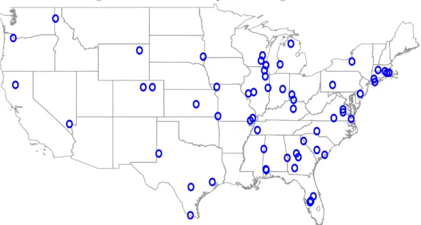
The database includes 982 non-cogeneration fossil-fuel plants larger than 100 megawatts. Of these, 60 were opened between 1991 and 1999 including 52 natural gas plants, six coal plants and two oil plants. Although the 1990s was a slow period of power plant construction compared to previous decades, this still represents a large sample of facilities compared to most hedonic studies, and a considerable improvement over Blomquist (1974) which examines a single power plant. Figure 1 provides a map indicating the locations of the plants. All geographic coordinates were verified using aerial photos from Google Maps.14
3.2 Demographic and Housing Characteristics
The demographic and housing characteristics used in the analysis come from restricted census microdata from the 1990 and 2000 decennial census. Demographic characteristics include household income, household size, family structure, educational attainment and race. Housing characteristics include type of home, age of home, number of bedrooms, acreage, and the number of units in the building, as well as reported housing value for homeowners and reported monthly rent for renters.15 These restricted data are accessed at a census research data center after having a project approved by the Census Bureau. The primary advantage of these data is their geographic detail. Whereas public-use microdata identify households at the PUMA, these restricted microdata identify households at the census block, the smallest geographic unit used by the Census Bureau. These
14
For 53 of the 60 plants high resolution photos were available and the geographic coordinates of the facility could be confirmed visually up to the nearest 1/1000 of a degree (about 10 feet). For the remaining plants high resolution photos were not available and the EPA’s coordinates could not be confirmed definitively. Still, the low resolution photos suggest that the coordinates are highly accurate. In many cases, despite the low resolution it was possible to visually discern the power plant. In other cases, the coordinates corresponded to locations along a river or other body of water, locations where power plants tend to be sited.
15
It would have been valuable to expand the analysis to include data from the 1980 census. The Census Bureau, however, completely redesigned census geography with the 1990 Census, making it difficult to make comparisons between the 1980 and 1990 census. Moreover, it was not until 1990 that the entire U.S. was divided into census blocks. In 1980, census blocks had been created for all incorporated places with a population greater than 10,000. These places included approximately 70% of the nation’s population and 7% of its land area. Furthermore, there are serious concerns about the reliability of the 1980 census block coding. By the Census Bureau’s own admission, the geographic coding in 1980 was replete with errors, omissions, and inconsistencies, particularly with regard to census blocks and block groups. See U.S. Census Bureau (1994), page 11-8.
data offer more detailed geographic detail even than is available in summary files 1 and 3, the most detailed publicly-available tabulations for the 1990 and 2000 census. Although basic neighborhood characteristics about population, age and race from the short-form survey are available at the block level for both 1990 and 2000, the more detailed information from the long-form survey including housing values, rents, and housing characteristics are available only at the block group level for 2000. The neighborhood impact from power plants is highly localized so this geographic detail is critical.
In addition to the increased geographic detail, microdata make it possible to control for housing unit-specific covariates, increasing the precision of the estimates. Still, it is important not to overstate the benefits of using microdata as opposed to the publicly-available tabulations. Although microdata would allow one, for example, to examine how changes in housing prices and rents vary across homes with different characteristics, this is not the focus here. Nor are these microdata being used to examine how MWTP varies across households with different observable characteristics as in Bayer, Ferreira, and McMillan (2007).
The last important advantage of using restricted data is the broad geographic coverage. Re-stricted data provide information for the full sample of households that filled out the long-form survey. In 1990 and 2000, this includes 1 in 6 households in the United States compared to the 5% sample available with public-use microdata. Moreover, the stratified sampling used by the Census Bureau ensures that even places with small populations are represented proportionally in the sample.16
The measures of housing values and rents in the census data are reported. With any self-reported information one may be concerned about whether or not households are able to answer accurately. Housing values are self-reported in response to a question that prompts respondents to report how much they think their home would sell for if it were for sale. Particularly for owners
16
In the 1990 census, 1 in 2 households were surveyed in places with population under 2,500 compared to 1 in 8 households elsewhere. In the 2000 census, 1 in 2 households were surveyed in places with fewer than 800 units, 1 in 4 households in places with fewer than 1200 units, 1 in 6 in places with fewer than 2000 units, and 1 in 8 elsewhere. An alternative to using census data would be to use the American Housing Survey. The advantage of the AHS is that it includes more detailed housing characteristics than the decennial census. However, the AHS does not have the geographical coverage or sample size available in the census. Most of the facilities examined in this study are not within the 47 metropolitan areas covered by the AHS. Also, during this period the AHS interviews approximately 55,000 households every other year, not enough households to be able to have broad coverage in the areas under consideration. Another alternative would be to use commercially available sales data. For example, DataQuick maintains an extensive database of housing sales based on public records from over 800 localities in 46 states including over 87 million total transactions. The advantage of sales data is that they are available at a high frequency. Sales data, however, are not a representative sample like the census data and typically rental prices are not available.
who purchased their homes many years ago, this may be difficult for some households to answer. In contrast, rent is presumably not subject to the same degree of misreporting as housing values because of the saliency of rent payments. Another potential problem with housing values is that they are reported for 20 different categories.17 In the empirical analysis housing value is treated as a continuous variable using the midpoint of the range. Again, rental rates are less problematic. In 1990 rent was categorical, but the number of categories was larger (26 categories), and in 2000 rent was a write-in response.
4
Empirical Strategy
4.1 The Omitted Variables Problem
In equilibrium, the price of housing near undesirable local facilities must be lower than the price of housing in other neighborhoods in order to attract households to these neighborhoods. In this paper, these equalizing differences are recovered by estimating a hedonic price function. Following Rosen (1974), the coefficients of the hedonic price function are interpreted as household MWTP for an incremental change in that attribute. In estimating this hedonic price function several econometric challenges must be addressed. Perhaps most importantly, there are unobserved differences between neighborhoods with power plants and neighborhoods without power plants. Siting decisions are likely to be correlated with local neighborhood and housing characteristics which are imperfectly observed. If these unobserved factors are also correlated with housing values then estimates of the hedonic price function will be biased.
Several different approaches have been used in recent hedonic studies to address this omitted variables problem. Chay and Greenstone (2005) measure the effect of air pollution on housing values using an instrumental variables approach exploiting variation in county-level air pollution induced by the Clean Air Act. Bayer, Keohane, and Timmins (2006) measure the effect of air pollution on housing values instrumenting for county-level particulate matter concentrations using distant emissions. Greenstone and Gallagher (2008) examine the effect of Superfund clean-ups using a regression discontinuity design, comparing housing values near clean-ups to housing values near sites that narrowly missed being cleaned up according the EPA’s selection rule. These papers all rely on plausibly exogenous variation in amenities to identify the effect of amenities on housing
17
In 1990 the highest category for housing values begins at $500,000 and in 2000 the highest category begins at $1,000,000. This change in categories is unlikely to influence the results, however, because only a tiny fraction of homes in the sample are in this highest category.
prices.
Another group of papers in this literature addresses the omitted variables problem by comparing before and after a change in amenities or before and after a change in information about amenities. For example, Kohlhase (1991) examines housing values before and after EPA announcements that a toxic waste site has been listed on the Superfund list. Kiel and McClain (1995) study the effect of a new garbage incinerator on housing values in Massachusetts. Gayer, Hamilton and Viscusi (2000) examine housing values near Superfund sites after information about the sites is released. These studies control for time-invariant neighborhood characteristics by focusing on changes in housing values over time. In some cases, a second location which did not experience the changes in amenities is used as a comparison group. For example, Davis (2004) examines housing prices in a county in Nevada before and after a cancer cluster, compared to changes in housing prices in a nearby county. Although this difference-in-differences approach offers advantages over a conventional cross-sectional analysis, it is not a panacea as is discussed below.
This paper addresses the omitted variables problem using this difference-in-differences approach. The study compares housing values and rents before and after plant openings to control for the unobserved characteristics of affected neighborhoods. In addition, the empirical strategy relies on highly localized comparisons across neighborhoods to control for time effects. In particular, homes far away from the site act as a comparison group for homes in the immediate vicinity. In the main specification, homes located within two miles of a power plant site are compared to homes located between two and five miles away.
4.2 The Baseline Specification
Equation (1) describes the hedonic price function estimated in the paper, logpricejt=α1xjt+ α21(within two miles)j ∗ 1(year 2000)t+
α31(year 2000)t∗ power plant site indicatorsj+
census block fixed effectsj+ ǫjt.
(1)
where j indexes individual houses and t indexes time. Equation (1) is estimated separately for home owners and renters. For home owners, the dependent variable, logprice, is the reported housing value (in logs). For renters, the dependent variable is the reported monthly rent (in logs). There are two time periods, 1990 and 2000.
Census block fixed effects are used to control for unobserved factors that are consistent over time. Although geographic boundaries changed for many census blocks between 1990 and 2000, the census bureau provides files that describe the relationship between 1990 and 2000 census blocks. These files were used to create geographic identifiers linking 1990 and 2000. For expositional simplicity these units will be referred to as census blocks and in cases where there is a one-to-one matching between census blocks in 1990 and 2000, these units are indeed census blocks. In cases where the relationship is one-to-many, many-to-one, or many-to-many, geographic identifiers correspond to the smallest consistent geographic unit across the two surveys.
The sample includes homes located within five miles of the nearest power plant site. The indicator variable 1(within two miles) indicates homes within two miles of the nearest power plant site. The restricted census microdata make it possible to highly accurately assign distances to homes based on the distance between the plant site and the census block centroid.18 Two miles is selected as the cutoff in the baseline specification because it is a large enough area to include the households most affected by local disamenities. Section 5.1 presents results from an alternative specification that allows MWTP to vary flexibly with distance to the plant.
The coefficient of interest, α2, is household MWTP to avoid living within two miles of an
operating power plant. This is the difference-in-difference estimate, the effect of power plants on housing prices, controlling for time and distance effects. The specification includes a variety of control variables. Housing characteristics are denoted xjt and include age of the home and
indicator variables for the number of bedrooms, number of units in the building, and whether or not the home has complete plumbing, one or more acres, and ten or more acres. The census block fixed effects control for unobserved neighborhood characteristics that do not change over time. For example, the census block fixed effects allow for the area in the immediate vicinity of the plant site to be different from the neighborhoods farther away, even prior to plant openings. In addition, the specification controls flexibly for time trends. In particular, the variable 1(year 2000) is interacted with indicator variables for each power plant site allowing the area around each power plant to have a different and unrestricted time trend between 1990 and 2000. This flexibility is important, for example, because of differential time trends by state and region. Finally, the estimating equation
18
There is some precedent in this literature for constructing neighborhoods using circles. In related work, Banzhaf and Walsh (2008) create half-mile circles by aggregating up from census block and block group level tabulations, finding evidence in high-toxic areas of out-migration of Whites and in-migration of Hispanics. Saha and Mohai (2005) create 1 mile radius circles around 23 hazardous waste facilities in Michigan and then use block group tabulations for 1980 and 1990 to infer the population and demographic characteristics within the radius. With their area weighting approach, population characteristics within each circle are assumed to be an area-weighted average of the block groups that intersect the circle.
includes ǫjt, an idiosyncratic component.
The strategy of examining plant openings makes it possible to control for time-invariant neigh-borhood characteristics and the estimates of α2 will be consistent even if the 5-mile-radius
“neigh-borhoods” are not perfectly homogenous. Least squares estimation of equation (1) is consistent if the interaction of 1(year 2000) and 1(within two miles) is exogenous conditional on housing characteristics, 1(year 2000) interacted with power plant indicators, and census block fixed effects,
E[ǫjt|xjt,1(within two miles)j∗ 1(year 2000)t,
1(year 2000)t∗ power plant site indicatorsj, census block fixed effectsj] = 0.
(2)
The primary source of potential correlation between ǫjt and the interaction term is
highly-localized differential time trends in housing prices and rents that are correlated with plant location decisions. For example, if power plants tend to be opened in locations that are in decline relative to the comparison neighborhoods, this would lead to estimates of MWTP that are biased away from zero. Still, it is worth emphasizing that the specification allows for separate time trends for each power plant site, thus controlling for regional, state, and local trends in housing values and rents. In addition, the advantage of using a comparison group that is close in physical proximity to the neighborhoods in the immediate vicinity of plants is that many factors that explain local housing market trends (e.g. changes in labor markets) are therefore controlled for.
The variance matrix is estimated taking into account that there are unobserved factors that cause prices to be correlated within power plant sites. An important advantage of the distance-based approach is that within the five mile radii considered in the analysis many factors such as school quality, local property taxes, and other factors are likely to be similar. However, even within these relatively small areas, and even after controlling for housing characteristics there are unobserved factors such as highly-localized geographical features and neighborhood amenities that cause nearby housing values to be correlated. Under this correlation, parameter estimates are still unbiased and consistent but the variance matrix must be corrected. Clustering by plant site allows each site to have a different and unrestricted covariance structure, but assumes that errors are uncorrelated across sites.
to neighborhoods near sites where plants opened before 1990 or after 2000.19 Since the process
by which plants are sited is not believed to have changed substantially during this period, these neighborhoods might have similar characteristics and trends compared to neighborhoods where plants opened during the 1990s. This approach is unlikely to provide a credible counterfactual, however, because plant openings before 1990 and after 2000 have direct effects on changes in housing values and rents between 1990 and 2000. Neighborhoods where plants opened before 1990 are not a credible comparison group because power plants permanently alter trends in housing values and rents by affecting neighborhood composition and subsequent decisions about whether or not to open additional industrial facilities. Also, plant utilization and other operating characteristics of existing plants change over time, affecting the desirability of local neighborhoods. Neighborhoods where plants opened after 2000 are not a credible comparison group because of anticipation effects. As discussed in the following section, plant openings require several years of planning. As a result, housing values in 2000 will already reflect expectations about future plant construction. In addition, neighborhoods where plants opened before 1990 or after 2000 come from different local markets. An advantage of the distance-based counterfactual is that the comparison group is in close geographic proximity making it possible to control for unobserved community-specific shocks.20
The approach used in the paper for estimating MWTP ignores mobility costs and general equilibrium effects. See Bayer, Keohane, and Timmins (2006) for a recent study that uses a discrete choice model to incorporate mobility costs into a neighborhood choice framework. Bayer, Keohane, and Timmins find estimates of MWTP for air quality that are three times larger than the estimates of MWTP they find when they estimate a conventional hedonic model using these same data. Discrete choice models have also been used to distinguish between partial equilibrium and general equilibrium effects. Sieg, Smith, Banzhaf, and Walsh (2005), for example, adopt a general equilibrium framework to measure the effect of air quality on housing values. This general equilibrium approach is particularly important for their application because air quality affects a large proportion of households. Relatively few households live near power plants so partial
19
This strategy has been used effectively in other contexts. For example, Busso and Kline (2008) use empowerment zones awarded in 1999 and 2001 as a point of comparison for empowerment zones awarded in 1994.
20
Furthermore, an alternative counterfactual using neighborhoods where plants opened before 1990 or after 2000 only makes sense if one believe that trends for a particular type of neighborhood are constant over time. Plant openings are endogenously determined at a particular point in time. Therefore, the fact that a plant was opened in one location in the 1980s and another in location in the 1990s suggests that these locations are not identical. Moreover, even if these neighborhoods have similar characteristics and trends at the time of openings, this does not imply that the neighborhoods will follow similar trends during the 1990s. Because of this concern and the other considerations raised in this section, it does not make sense to perform a false experiment with neighborhoods with plants that opened before 1990 or after 2000.
equilibrium effects are likely to provide a reasonable approximation to general equilibrium effects.
4.3 Examining Where Power Plants Were Opened During the 1990s
This section examines the neighborhoods where power plants were opened during the 1990s. Household demographic and housing characteristics are examined in 1990, before the plants were opened, comparing households living near plant sites with households living farther away. These descriptive statistics are valuable because they provide information about the siting process for plants and because they provide evidence on the validity of these farther away neighborhoods as a comparison group.
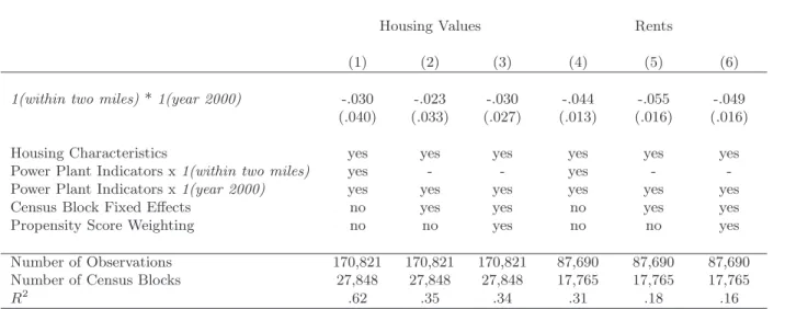
Table 1 reports mean household demographic and housing characteristics in 1990 for households living within two miles of plant sites, households living between two and five miles of plant sites, and households in the entire United States. The table also reports p-values from tests of equal means. The table indicates that neighborhoods within two miles of the plant sites are different, both from the neighborhoods two to five miles from the sites and from the United States as a whole. For example, household income in the neighborhoods within two miles is lower than household income in the other two groups and the differences are highly statistically significant. Within two miles households tend to have more children and household heads are less likely to have finished high school. In addition, the proportion of households for which the household head is Black or Hispanic in the neighborhoods within two miles is higher than the proportion in the two to five mile neighborhoods or in the United States as a whole. This is consistent with evidence from a substantial environmental justice literature (see, e.g., Been 1994, Oakes, Anderton and Anderson 1996, Been and Gupta 1997, Helfand 1999, and Saha and Mohai 2005). Compared to the United States as a whole, the null hypothesis of equal means is rejected in all 20 cases. Compared to the two to five mile neighborhoods, equal means are rejected at the 1% level in 16 out of 20 cases. In part, these rejections reflect the large sample size. However, even when alternative critical values are adopted following Leamer (1978) that account for sample size the null of equal means continues to be rejected in most cases.
Despite these differences the two to five mile group is still a valuable comparison group because of its geographic proximity to the within two mile group. Many of the factors that explain local housing market trends (e.g. changes in labor markets) are likely to be similar within these relatively small geographic areas. As discussed in section 4.2, the estimates of MWTP will be unbiased as long as, controlling for observables and census block fixed effects, the trends in housing prices are
the same in the two to five mile neighborhoods as they would have been in the zero to two mile neighborhoods.
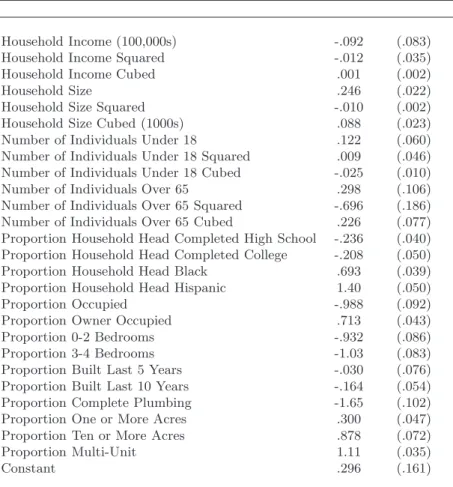
Column (4) reports covariate means weighted by propensity scores. The idea of propensity score weighting is to reweight the observations in the two to five mile group to balance the co-variate means with the zero to two mile group, increasing the weight assigned to households that are similar to households in the immediate vicinity of plants. First, census block averages are created for all covariates. Second, propensity scores are estimated using a logit regression with 1(within two miles) as the dependent variable and independent variables including all variables in table 1 except for housing values and rents. Cubics are used for all variables that are not propor-tions (household income, household size, number of children, and number of individuals over 65). Estimated coefficients and standard errors from the propensity score logit regression are reported in Table A1. Third, following Rosenbaum (1987) the propensity scores from this regression are used to reweight the observations in the two to five mile group by the relative odds, p(xjt)
1−p(xjt), where p(xjt) is the propensity score (i.e. the conditional probability of being in the zero to two mile group
given covariates).21
The propensity score weighting substantially balances covariate means across the within two mile and two to five mile groups. Means for all covariates are similar in magnitude and the null hypothesis of equal means can be rejected at the 1% significance level in only two out of 20 cases. The reweighting specification reduces the potential scope for functional form mispecification in the estimating equation to bias the results. In addition, this reweighting helps address potential concerns about differential time trends. The results presented in the following section allow the area around each power plant site to have a different time trend. If, in addition, there are highly-localized trends within these neighborhoods that lead the within two mile group to have a different time trend from the two to five mile group, this is addressed in the propensity score weighting specification to the extent that these differential trends are explained by observables. For example, if trends in housing values and rents vary across census blocks with different levels of household income, the propensity score weighting specification controls for this by balancing average household income across the two groups.
21
The following section reports results from estimating equation (1) using these weights. The standard errors reported for this specification do not account for the variance component due to estimation of the propensity scores. The coefficients in the logit regression are precisely estimated, however, so the magnitude of the potential bias is small. See Pagan (1984) and Murphy and Topel (1985) for discussion of inference in models with generated regressors.
5
Results
5.1 Estimates of MWTP to Avoid Living Near a Power Plant
Table 2 presents least squares estimates of the hedonic price function, equation (1). For all specifications the table reports the coefficient and standard error corresponding to the interaction between 1(within two miles) and 1(year 2000). All specifications include housing characteristics and power plant specific time trends. In column (1), the estimated household MWTP associated with living within two miles of an operating power plant is −.030, or 3.0% of housing values. Results for rents are similar, providing an important test of the robustness of the results. When the dependent variable is monthly rent in logs, column (4), the estimated MWTP is −.044. Columns (2) and (5) report results from a specification with census block fixed effects. Results are similar in this richer specification, with estimates of MWTP equal to −.023 for housing values and −.055 for rents. Columns (3) and (6) report results from the propensity score weighting specification. Results are similar to the results from the two previous specifications. Overall, point estimates for household MWTP to avoid living near a fossil-fuel power plant range from 2.3 − 3.0% for housing values and from 4.4 − 5.5% for rents.
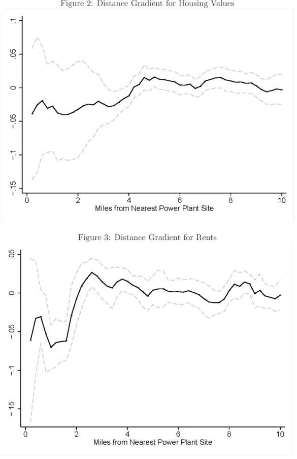
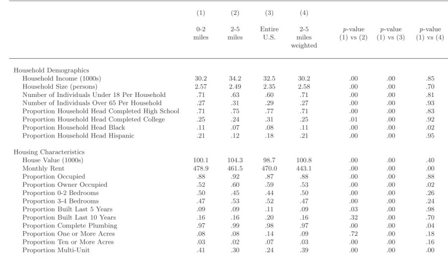
Figures 2 and 3 describe the gradient of housing values and rents with respect to distance to the nearest power plant site. These figures were constructed using the census block fixed effects specification described in table 2, columns (2) and (5). For each figure fifty separate regressions were performed. In place of the interaction term 1(within two miles) ∗ 1(year 2000), each regres-sion included an interaction term of 1(year 2000) with an indicator variable corresponding to a different 1-mile wide distance from the plant. For example, the point estimates for one mile in figures 2 and 3 correspond to the coefficient and standard error corresponding to the interaction 1(between .5 and 1.5 miles) ∗ 1(year 2000). Thus, the specification allows MWTP to avoid living near an active power plant to vary flexibly by distance to the plant. The figure was constructed using all homes located within ten miles of the nearest plant, making it possible to evaluate the validity of the two to five mile group as a comparison group.
The results in figures 2 and 3 are consistent with the results reported in table 2. For housing values, point estimates for MWTP are negative and between -.03 and -.04 between zero miles and two miles, then increasing gradually to zero between three and four miles from the nearest plant site. For rents, there is a negative and statistically significant impact within two miles, increasing to zero beyond two miles. These results suggest that minor changes in the definitions of the treatment
and comparison groups would not meaningfully change the results presented in table 2.
Figures 2 and 3 also address possible concerns about contamination of the comparison group. Even in the absence of a significant direct effect, property values and rents in the two to five mile neighborhood might have been affected indirectly by household mobility. Suppose power plants cause household to move out of neighborhoods in the immediate vicinity of the plant, but labor market and other considerations make it undesirable for these households to move far away. Increased demand for housing in the two to five mile neighborhood would cause the cost of housing to increase, potentially biasing the estimates of MWTP away from zero. Based on the evidence in figures 2 and 3, this does not appear to be the case. The estimated coefficients between two miles and ten miles are close to zero and not statistically significant for both housing values and rents, suggesting that contamination of the comparison group is not driving the results.
It is valuable to compare the estimated coefficients in this section with estimates of MWTP from previous studies. Chay and Greenstone (2005) find that the elasticity of housing values with respect to particulates concentrations ranges from −.20 to −.35 so that, for example, the 11 − 12% reduction in TSPs they observe in non-attainment counties is associated with a 2 − 3.5% increase in housing values. Bayer, Keohane, and Timmins (2006) find somewhat larger elasticities, −.34 to −.42, using a discrete-continuous approach that accounts for mobility costs. Greenstone and Gallagher (2008) find smaller point estimates, −.008 to .018, for homes within a 2-mile radius of hazardous waste clean-ups.
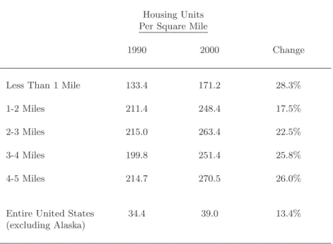
There are on average, 2900 housing units within two miles of each power plant site.22 The mean housing value from table 1 implies that the average total value of the housing stock within two miles of a plant site is $483 million in year 2008 dollars. Multiplying this by the estimate of MWTP from column (3) yields an average housing market capitalization within two miles of a plant of $14.5 million. As a point of comparison, recall that the typical cost of a large capacity (435 kilovolt) transmission line is $800, 000 per mile.23 In some cases, moving a plant one or two miles in one direction or another would substantially reduce the size of the affected nearby population. In other cases, plants are in highly-populated areas and it would require many mile of additional transmission (and siting of transmission lines) in order to reduce the size of the affected nearby population. As described in section 2.2, policymakers must take many different factors into account
22
Table A2 in the appendix reports housing units per square mile near plant openings for various distances. See Greenstone and Gallagher (2008) for a discussion of the response of housing supply to changes in environmental amenities.
23
when deciding whether or not to approve power plant proposals including local disamenities and transmission costs. These estimates of the social cost of local disamenities provide a benchmark for formally incorporating local disamenities into the cost-benefit analysis.
This measure understates the total value of local disamenities because it reflects residential property, but not industrial, commercial, or undeveloped property. While some industrial uses may not be substantially impacted by power plant proximity, commercial property, and perhaps more importantly, undeveloped property, will certainly be affected. When making policies that affect power plant siting, policymakers should consider the costs imposed to all agents. In addition, this measure of the average housing market capitalization per plant obscures the fact that there are large differences across plants in the implied market capitalization. Some power plants that opened during the 1990s are located in almost completely uninhabited areas whereas other plants were opened in highly-populated areas. The results imply that the distribution of market capitalization across sites is right skewed with a small number of sites responsible for a large amount of total market capitalization. This is not, in itself, evidence that these plants would not pass a cost-benefit test because plant siting depends on many factors. However, it does illustrate that there can be large differences in the social cost of disamenities across sites.
5.2 Alternative Specifications Using Subsets of Plants
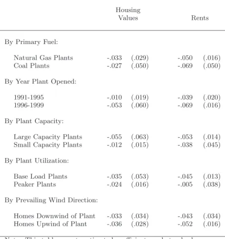
Table 3 reports least squares estimates of MWTP for 20 separate regressions, each using a par-ticular subset of power plant sites or households. For each regression the table reports the estimated coefficient and standard error corresponding to the interaction 1(within two miles) ∗ 1(year 2000). All specifications are weighted by propensity scores and include housing characteristics, census block fixed effects, and separate time trends for each power plant site as in table 2, columns (3) and (6).
First, the table reports estimates separately for plants that use natural gas and plants that use coal. During the 1990s there was a pronounced shift in plant construction away from coal toward natural gas and this specification is relevant for evaluating the welfare consequences of this change. At current prices there is a substantial cost advantage for coal.24 However, coal plants
tend to emit higher levels of pollutants and have other differential impacts on local communities, and it is important to consider these differences when making policy which affects this tradeoff.
24
In 2005, the average cost for coal-based electricity generation was $1.54 per million Btu compared to $6.44 for fuel oil and $8.21 for natural gas. See U.S. Department of Energy (2007), Table 4.5.
The estimates for both types of plants are similar in magnitude to the baseline MWTP estimates reported in table 2 and the estimates provide no evidence that MWTP differs by plant type. It is difficult to draw definitive conclusions, however, because the standard errors for coal plants are large, reflecting the fact that there were relatively few coal plants opened during the 1990s.
Second, the table reports estimates of MWTP separately for plants that opened during 1991-1995 and plants that opened between 1996 and 1999. This alternative specification addresses possible concerns about timing. Whereas information about plant openings during the early 1990s was likely available in 1990, openings in the late 1990s are unlikely to have been capitalized into housing values in 1990. For both housing values and rents the point estimates are larger for plants opened later in the decade, consistent with these anticipation effects.
Third, the table reports estimates of MWTP separately by plant capacity. Large capacity plants are those for which the nameplate capacity exceeds 275 megawatts, the median nameplate capacity in the dataset. The results are consistent with large capacity plants having a larger associated MWTP, though the differences are not statistically significant. Point estimates for large capacity plants are 5.5% for housing values and 5.3% for rents, compared to 1.2% and 3.8% for small capacity plants.
Fourth, the table reports estimates separately by plant utilization. High utilization plants are those for which the capacity factor exceeds .15, the median capacity factor in the dataset, where capacity factor is the ratio of plant net generation to nameplate capacity. Again the results are consistent with what would be expected with high utilization plants associated with larger disamenities. For example, for rents, the estimated coefficient for high utilization plants is −.045 compared to a point estimate near zero for low utilization plants.
Fifth, the table reports estimates separately for upwind and downwind households.25 The
sample was divided into two subsets based on prevailing wind direction. Downwind households were defined as homes for which the bearing between the power plant and the home was within 45 degrees of the prevailing wind direction. The results are similar for the two subsets, providing no evidence of a disproportionate impact on homes downwind of plants. These findings are consistent with the description of plants in section 2.1, that emphasizes that local externalities from power plants include not only air quality effects, but also traffic, visual disamenities, and other disamenities that affect households both upwind and downwind.
25
Prevailing wind direction comes from the U.S. Department of Commerce (1998) for 321 locations in the United States summarizing over 60 years of data from weather stations. The prevailing wind direction for each plant site is determined using the closest available weather station.
There are undoubtedly additional alternative specifications that would be valuable to exam-ine. One alternative, for example, would be to estimate and report MWTP separately by plant. However, this specification does not meet Census disclosure requirements which prevent reporting coefficients based on a small number of households.26
In addition to describing MWTP for different potentially important subsets, these alternative specifications also serve as an important test of the robustness of the full sample results in the pre-vious section. Although it is impossible to rule out the possibility that differential highly-localized time trends are influencing the results, the robustness of the results across multiple specifications is reassuring. In order to explain the results with differential time trends, not only would one need differential decreases in neighborhoods in the immediate vicinity of where plants open, but these trends would need to hold for both housing values and rents, and hold for the different subsamples. To explain the results by plant capacity, for example, one would need stronger differential time trends for neighborhoods near large capacity plants.
The results from these alternative specifications also assuage concerns about the results being driven by broader changes in siting patterns. In particular, one could imagine highly-localized changes in the political climate that would make it easier to site power plants and other types of undesirable industrial facilities at the same time. Similarly, one might be concerned that power plant siting might affect subsequent decisions about where to site other types of industrial facilities, leading to a cluster of nearby facilities. Under these scenarios, the estimates of MWTP would be biased away from zero because they would reflect the disamenities from multiple facilities. Again, although it is impossible to rule out these possibilities, the fact that the estimates of MWTP respond somewhat predictably across plant type lends support to the idea that these estimates are capturing the impact of power plants, rather than the impact of other facilities that are correlated with power plant openings.
6
Conclusion
Electricity consumption in the United States is forecast to continue to increase over the next several decades. Although wind, solar, and other alternative sources of electricity production receive a great deal of attention from policymakers, the low cost of fossil-fuel electricity generation all but
26
Another potentially valuable specification would be to compare plants with different types of nitrogen oxides or sulfur dioxide control devices. However, relatively few plants that opened during the 1990s have selective catalytic reduction or scrubbers. In addition, the plants with control devices tend to be large capacity plants, making it difficult to disentangle the effect of these control devices from the effect of plant size.
guarantees that it will play a central role in meeting this growing demand. At the same time, siting of power plants has become more difficult than ever, in large part because the need for new facilities is most severe in places with large and growing populations. Policymakers face difficult, often politically contentious decisions about where to site plants balancing many different factors. Although local amenities are typically one of the important factors considered in this process, the lack of reliable empirical evidence about the magnitude of these costs has prevented the use of cost-benefit analysis.
This paper is the first large-scale effort to assess the value of local disamenities from power plants. Focusing on neighborhoods in the immediate vicinity of plants, the empirical analysis ex-ploits plant openings to mitigate concerns about omitted variables and sorting. An integral feature of the analysis is the use of restricted census microdata. Although not without its limitations, these data provide a level of geographic detail and sample size that is not available anywhere else. The results provide a rich description of the impact of power plants on housing markets. Relative to neighborhoods farther away, housing values and rents decrease by 3 − 5% when plants open, imply-ing an average housimply-ing market capitalization within two miles of a plant of $14.5 million. Estimates of MWTP respond predictably across a variety of alternative specifications. For example, MWTP is larger for large capacity plants and for plants opened late in the decade. These estimates provide a benchmark for formally incorporating local disamenities into decisions about where plants are sited.
References
[1] Bayer, Patrick, Fernando Ferreira, and Robert McMillan. “A Unified Framework for Measuring Prefer-ences for Schools and Neighborhoods.” Journal of Political Economy, 2007, 115(4): 588-638.
[2] Bayer, Patrick, Nathaniel Keohane, and Christopher Timmins. “Migration and Hedonic Valuation: The Case of Air Quality.” working paper, 2006.
[3] Banzhauf, H. Spencer, Randall P. Walsh. “ Do People Vote with their Feet?: An Empirical Test of Environmental Gentrification.” American Economic Review, forthcoming, 2008.
[4] Blomquist, Glenn. “The Effect of Electric Utility Power Plant Location on Area Property Value.” Land Economics, 1974, 50(1): 97-100.
[5] Busso, Matias and Patrick Kline. “Do Local Economic Development Programs Work? Evidence from the Federal Empowerment Zone Program.” working paper, 2008.
[6] California Energy Commission. “Rules of Practice and Procedure – Power Plant Site Certification Regulations.” April 2007, CEC-140-2007-003.
[7] California State Auditor. “California Energy Commission: Although External Factors Have Caused Delays in Its Approval of Sites, Its Application Process is Reasonable.” August 2001, 2001-118. [8] Chay, Kenneth Y. and Michael Greenstone. “Does Air Quality Matter? Evidence from the Housing
Market.” Journal of Political Economy, 2005, 113(2), 376-424.
[9] Davis, Lucas W. “The Effect of Health Risk on Housing Values: Evidence from a Cancer Cluster.” American Economic Review, 2004, 94(5), 1693-1704.
[10] Edison Electric Institute. “State Generation and Transmission Siting Directory: Agencies, Contacts, and Regulations.” Washington, D.C., 2004.
[11] Epple, Dennis and Allan Zelenitz. “The Implications of Competition Among Jurisdictions: Does Tiebout Need Politics?” Journal of Political Economy, 1981, 89(6), 1197-1217.
[12] Gamble, H.B. and R.H. Downing. “Effects of Nuclear Power Plants on Residential Property Values.” Journal of Regional Science, 1982, 22(4): 457-478.
[13] Gayer, Ted, James T. Hamilton and W. Kip Viscusi. “Private Values of Risk Tradeoffs at Superfund Sites: Housing Market Evidence on Learning About Risk.” Review of Economics and Statistics, 2000, 82(3), 439-451.
[14] Greenstone, Michael and Justin Gallagher. “Does Hazardous Waste Matter? Evidence from the Housing Market and the Superfund Program.” Quarterly Journal of Economics, forthcoming, 2008.
[15] Hirst, Eric and Brenan Kirby. “Transmission Planning and the Need for New Capacity.” U.S. Depart-ment of Energy, 2002, Washington, DC.
[16] Kahn, Matthew E. “Population Change Near Polluting Power Plants: Implications for the Social Cost of Power Generation.” working paper, 2007.
[17] Kiel, K. and K. McClain. “House Prices during Siting Decision Stages: The Case of an Incinerator from Rumor through Operation.” Journal of Environmental Economics and Management, 1995, 28, 241-255. [18] Kohlhase, Janet E. “The Impact of Toxic Waste Sites on Housing Values.” Journal of Urban Economics,
1991, 30, 1-26.
[19] Leggett, Christopher G. and Nancy E. Bockstael. “Evidence of the Effects of Water Quality on Resi-dential Land Prices.” Journal of Environmental Economics and Management, 2000, 39(2), 121-144. [20] Mauzerall, Denise L., Babar Sultan, Namsoug Kim and David F. Bradford. “NOx Emissions from Large
Point Sources: Variability in Ozone Production, Resulting Health Damages and Economic Costs.” Atmospheric Environment, 2005, 39: 2851-2866.
[21] Muller, Nicholas Z. and Robert Mendelsohn. “Efficient Pollution Regulations: Getting the Prices Right.” 2007, working paper, Middlebury College and Yale University.
[22] Leamer, Edward E. Specification Searches: Ad hoc Inference with Nonexperimental Data, New York: Wiley-Interscience, 1978.
[23] Levy, Jonathan I., John D. Spengler, Dennis Hlinka, David Sullivan, and Dennis Moon. “Using CALPUFF to Evaluate the Impacts of Power Plant Emissions in Illinois: Model Sensitivity and Impli-cations.” Atmospheric Environment, 2002, 36: 1063-1075.
[24] Levy, Jonathan I. and John D. Spengler. “Modeling the Benefits of Power Plant Emission Controls in Massachusetts.” Air and Waste Management, 2002, 52: 5-18.
[25] Murphy, Kevin M. and Robert H. Topel. “Estimation and Inference in Two-Step Econometric Models.” Journal of Business and Economic Statistics, 1985, 3(4), 370-379.
[26] National Research Council. “Managing Coal Combusion in Mines.” National Academies Press, Wash-ington D.C., 2006.
[27] Nelson, Jon P. “Three Mile Island and Residential Property Values: Empirical Analysis and Policy Implications.” Land Economics, 1981, 57(3), 363-372.
[28] Oates, Wallace E. and Robert M. Schwab. “Economic competition among jurisdictions: efficiency en-hancing or distortion inducing?” Journal of Public Economics, 1988, 35(3), 333-354.
[29] Pagan, Adrian. “Econometric Issues in the Analysis of Regressions with Generated Regressors.” Inter-national Economic Review, 1984, 25(1), 221-232.
[30] Rosen, Sherwin. “Hedonic Prices and Implicit Markets: Product Differentiation in Pure Competition.” Journal of Political Economy, 1974, 82, 34-55.
[31] Rosenbaum, Paul. Model-Based Direct Adjustment. Journal of the American Statistical Association, 1987, 82(398), 387-394.
[32] Saha, Robin and Paul Mohai. “Historical Context and Hazardous Waste Facility Siting: Understanding Temporal Patterns in Michigan.” Social Problems, 2005, 52(4): 618-648.
[33] Sieg, Holger, V. Kerry Smith, H. Spencer Banzhaf and Randy Walsh. “Estimating the General Equilib-rium Benefits of Large Changes in Spatially Delineated Public Goods.” International Economic Review, 2004, 45(4), 1047-1077.
[34] U.S. Census Bureau. “Geographic Areas Reference Manual.” November 1994.
[35] U.S. Department of Commerce, National Oceanic and Atmospheric Administration. “National Climatic Data Center: Climatic Wind Data for the United States.” November 1998.
[36] U.S. Bureau of Labor Statistics, U.S. Department of Labor. “Occupational Outlook Handbook, 2008-09 Edition, Power Plant Operators, Distributors, and Dispatchers.” 2008.
[37] U.S. Department of Energy. “Electric Power Annual 1994.” July 1995, DOE/EIA-0348.
[38] U.S. Department of Energy.“Annual Energy Outlook 2007.” February 2007 (2007a), DOE/EIA-0383. [39] U.S. Department of Energy. “Electric Power Annual 2006.” November 2007 (2007b), DOE/EIA-0348. [40] U.S. Department of Health and Human Services. “ToxFAQs.” 2007.
[41] U.S. Environmental Protection Agency. “The Particle Pollution Report: Current Understanding of Air Quality and Emissions through 2003.” December 2004, EPA 454-R-04-002.
[42] U.S. Environmental Protection Agency. “Waste and Materials-Flow Benchmark Sector Report: Benefi-cial Use of Secondary Materials - Coal Combustion Products.” February 2008.
[43] U.S. Environmental Protection Agency. “Mercury Study Report to Congress, Volume III: Fate and Transport of Mercury in the Environment.” December 1997, EPA 452-R-97-005.
[44] Vajjhala, Shalini P. and Paul S. Fischbeck. “Quantifying siting difficulty: A case study of U.S. trans-mission line siting.” Energy Policy, 2007, 35: 650-671.
Figure 2: Distance Gradient for Housing Values