Carbon Efficient Network Design: Evaluating The Trade-Offs Between Carbon Emissions, Transportation Cost and Delivery Time For a Middle-Mile Distribution Network

(1)

1

Carbon Efficient Network Design:

Evaluating the Trade-Offs Between Carbon Emissions, Transportation Cost,

and Delivery Time for a Middle-Mile Distribution Network

by

Ars-Vita Alamsyah

Bachelor of Science in Mechanical Engineering, University of Maryland, 2017 and

Namuun Purevdorj

Bachelor of Arts in International Relations, Mount Holyoke College, 2015

SUBMITTED TO THE PROGRAM IN SUPPLY CHAIN MANAGEMENT IN PARTIAL FULFILLMENT OF THE REQUIREMENTS FOR THE DEGREE OF

MASTER OF APPLIED SCIENCE IN SUPPLY CHAIN MANAGEMENT AT THE

MASSACHUSETTS INSTITUTE OF TECHNOLOGY

June 2021

The authors hereby grant to MIT permission to reproduce and to distribute publicly paper and electronic copies of this capstone or thesis document in whole or in part in any medium now

known or hereafter created.

Signature of Author: ____________________________________________________________ Ars-Vita Alamsyah Department of Supply Chain Management

May 14, 2021

Signature of Author: ____________________________________________________________ Namuun Purevdorj Department of Supply Chain Management

May 14, 2021

Certified by: __________________________________________________________________ Dr. Alexis Bateman Director and Research Scientist, MIT Sustainable Supply Chains Capstone Advisor

Accepted by: _________________________________________________________________ Prof. Yossi Sheffi Director, Center for Transportation and Logistics Elisha Gray II Professor of Engineering Systems Professor, Civil and Environmental Engineering

(2)

2

Carbon Efficient Network Design:

Evaluating the Trade-Offs Between Carbon Emissions, Transportation Cost,

and Delivery Time for a Middle-Mile Distribution Network

by

Ars-Vita Alamsyah and Namuun Purevdorj

Submitted to the Program in Supply Chain Management

on May 14, 2021 in Partial Fulfillment of the Requirements for the Degree of Master of Applied Science in Supply Chain Management

at the

Massachusetts Institute of Technology

ABSTRACT

The transportation sector is the third largest contributor to greenhouse gas (GHG) emissions, accounting for over 28% of total U.S. emissions and over 14% of global emissions in 2018. As climate change and its negative effects have grown significantly, efforts to reduce GHG emissions have become an important objective on a global, national, and corporate scale. One approach is to design a distribution network that minimizes transportation carbon emissions while meeting its primary Key Performance Indicators (KPI). It is important for companies to understand the trade-offs between those KPIs, which may include minimizing the carbon footprint, minimizing transportation costs, and meeting the network's delivery time requirements. This research introduces a multi-echelon Green facility location problem (FLP) that focuses on the middle-mile. It incorporates intermodal and alternative-fuel transportation modes and optimizes for the tri-objective of variable transportation cost, delivery time and carbon emissions. By using the ɛ-constraint method, Pareto frontiers for carbon emissions vs. cost and carbon emissions vs. delivery time were plotted, providing the trade-offs between objectives. Optimal scenarios on the Pareto frontiers were identified to align with 1.5o_{C and well-below 2}o_{C global climate scenarios}

according to the Science-Based Targets initiatives. The research team found that the trade-offs between carbon emissions vs. delivery time are non-linear and much more significant than carbon emissions vs. transportation variable cost. In order for firms to reach Science-Based Targets, it is necessary for companies that have transportation heavy operations with short delivery timelines to shift all transportation to vehicles powered by lower carbon fuels. This research informs the approach to start incorporating environmental considerations in the strategic decision-making process for supply chain network design.

Capstone Advisor : Dr. Alexis Bateman

Title : Director and Research Scientist, MIT Sustainable Supply Chains

Capstone Co-Advisor : Suzanne Greene

(3)

3

ACKNOWLEDGEMENTS

First and foremost, we would like to thank our advisor, Dr. Alexis Bateman for her guidance and support throughout the development of this research. We would also like to thank our co-advisor, Suzanne Greene for her direction and invaluable insights into carbon accounting. Thank you both for encouraging us to go the extra mile and providing us with the necessary tools and resources. We have learned so much about sustainable supply chains and its importance.

To the entire MIT Supply Chain Management faculty and staff who have been very accommodating in facilitating thoughtful discussions and providing input on network design and optimization - thank you. Special thanks to Josué Velázquez Martínez for your critical guidance in our methodology, as well as Toby Gooley and Pamela Siska for providing feedback on our report writing.

We thank our external stakeholders from the sponsoring company and Llamasoft. Thank you for the opportunity to collaborate in solving the complex supply chain problems that truly matter. We wish to especially thank the following individuals: Dan Kogan, Ryan Purcell, Gary Strickler, Kanchana Nanduri, Marco Ugarte, and Chris Atkins.

Last but not least, to the beloved family members and friends who have continuously offered support along this journey.

I am utterly grateful to have a supportive family that inspires me to pursue advanced degree and they have been my motivation to excel every single day. To my late grandparents, especially Aki Edi, MIT has been your dream in one of your last messages, and here I am as the first in the family. To my entire family members, thank you is an understatement. Your prayers, regular check-ins, and endless support are all matters which I cannot describe it one by one. Alhamdulillah, JazākAllāhu Khayran.

- Ars-Vita Alamsyah

I wish to thank my husband, Ganzo, for his love, patience, and for being my rock. This year of learning would not have been possible without you. My daughters, Ariulan and Eneren, thanks for putting up with my long “work” days and fueling me every day with your infectious joy. To my parents, Puje and Amaraa, for their continuous support, wisdom, and prayers. Thank you for teaching me to persevere and reach for the stars. To my best friend, Angelica, thank you for your never-ending encouragement.

(4)

4

LIST OF FIGURES

Figure 1. Historical Transportation Sector GHG Emissions in the United States Figure 2. Middle-Mile Distribution for the Transportation Network

Figure 3. GLEC Framework’s Carbon Emissions Calculation Scopes Figure 4. The Fuel Life Cycle for Carbon Accounting

Figure 5. On-The-Road Delivery Time Calculation Example Figure 6. Ports and inland waterways in the US

Figure 7. Connection Constraint on One IXD to a group of FC Constraint Figure 8. Intermodal Calculation Simplification

Figure 9. Total Transportation Cost at the Extreme Boundaries Figure 10. Total Carbon Emissions at the Extreme Boundaries

Figure 11. Total On-the-Road (OTR) Delivery Time at the Extreme Boundaries

Figure 12. Pareto Frontier for Baseline Model on Carbon Emissions vs. Transport Cost Figure 13. Pareto Frontier for Future Models on Carbon Emissions vs. Transport Cost Figure 14. Pareto Frontier for Baseline Model on Carbon Emissions vs. OTR Delivery Time Figure 15. Pareto Frontier for Future Model on Carbon Emissions vs. OTR Delivery Time Figure 16. Science Based Target Scenarios Identified on Carbon Emissions vs. Transport Cost

Pareto Frontier

Figure 17. Science-Based Target Scenarios Identified on Carbon Emissions vs. Delivery Time Pareto Frontier

Figure 18. Network Design for the Targeted Carbon Emissions Scenario at 1.5oC

Figure 19. Total Transportation Costs at the Extreme Boundaries for IXD-FC-SC-Customer Node Network

(7)

7

LIST OF TABLES

Table 1. Data Provided from MMTN

Table 2. Capacity Constraint as Number of Packages Per Day Table 3. Summary of Network Design Models

Table 4. Summary of Candidate Locations

Table 5. Science-Based Target Setting Tool - Scope 3 Targets Generated

Table 6. Vehicle Utilization for Carbon Emissions Level at 1.5oC and Well Below 2oC Table 7. Carbon Intensity for Science-Based Target Scenarios

Table 8. Variable Cost Per Ton Carbon Emissions Produced on Baseline Scenario model Table 9. Increase in Variable Cost Per Ton Carbon Emissions Decrease at 1.5o_{C Scenario}

Table 10. Average On-The-Road Delivery Time and CO2e Difference by Target Scenarios

Table 11. Average fill rates and carbon intensity factors for current transportation types Table 12. Average fill rates and carbon intensity factors for alternative transportation types Table 13. Transportation Modes Summary

Table 14. Intermodal Transportation Considerations Table 15. US National Average Fuel Price

Table 16. Data Required for Science-Based Target Setting Tools

Table 17. Baseline Data Inputs for the Target Setting Tool - Transport Sector

Table 18. Targets Generated for Minimum Emissions Baseline by Science-Based Target Setting Tool - Transport Sector

(8)

8

1. Introduction

1.1 Motivation for the Study

Traditionally, supply chain network design has focused on economic objectives. However, as climate change is occurring and concerns over its effects have grown significantly over the past few decades, environmental objectives have become an important consideration in supply chain decisions.

The transportation sector is not only vital for supply chains and the global economy but also the third largest contributor of greenhouse gas (GHG) emissions (International Energy Agency, 2019). At the current pace of economic growth, emissions from the transportation sector are set to double by 2050 (ITF, 2019). In 2018, the Intergovernmental Panel on Climate Change (IPCC) warned that it is not possible to avoid catastrophic impacts of climate change if global warming exceeds 1.5oC above pre-industrial1 temperatures. Since carbon emissions, a shorthand for GHG emissions, is the leading cause of global warming, efforts to estimate, track and reduce its release in the atmosphere have become integral for global-, government- and corporate-level sustainability goals.

Figure 1

Historical Transportation Sector GHG Emissions in the United States. Source: Climate Watch, 2019.

1_{The multi-century period prior to the onset of large-scale industrial activity around 1750. The reference period}

(9)

9

On a global scale, in 2015, 196 countries adopted the Paris Agreement, a legally binding international treaty that’s part of the United Nations (UN) Framework to fight climate change. Over the long term, the universal agreement aims to limit the increase in global temperatures to well below 2oC, and preferably to 1.5oC compared to pre-industrial levels (United Nations, 2015). In addition, methodologies and standards to measure and report carbon emissions have been established through joint initiatives between international organizations, governments and corporations. The Greenhouse Gas Protocol (GHGP) Corporate Standard as well as the Global Logistics and Emissions Council (GLEC) Framework are the main carbon accounting methodologies utilized by businesses to quantify their carbon emissions. The Carbon Disclosure Project (CDP), however, serves as the leading reporting platform for enterprise emissions, providing and acknowledging the increasing transparency of participating organizations’ carbon emissions accounting and reduction. The CDP along with the UN Global Compact, World Resources Institute (WRI), and the World-Wide Fund for Nature (WWF) partnered to create the Science-Based Targets initiative (SBTi). The initiative provides tools that help businesses world-wide set carbon emissions reduction targets that are in line with the climate goals of limiting global warming to 1.5oC.

In the United States, the transportation sector is the largest contributor to GHG emissions, which accounted for 28.2% in 2018 (Office of Transportation and Air Quality, 2020). Light-duty vehicles, medium- and heavy-Light-duty trucks, and airplanes are among the top three modes of transportation that contribute to GHG emissions - 59%, 23%, and 9%, respectively (Office of Transportation and Air Quality, 2020). Given this fact, stakeholders in logistics and transportations have started to locally strategize and implement policies to achieve these global goals. The United States has set goals of progressively reducing carbon emissions by 50 to 52% by the end of 2030, and reaching net zero carbon emissions by no later than 2050, compared to the emissions level in 2005 (The United States Government, 2021). Past efforts at the national level include President Obama’s Climate Action Plan, bills on renewable energy utilization, and GHGs inventory regulation by states. Policies at different levels help all stakeholders to participate and navigate actions to take.

On a corporate level, companies such as Middle-Mile Transportation Network (MMTN), have joined initiatives such as The Climate Pledge that call organizations globally to implement measures that combat climate change. MMTN has pledged to reduce 50% of its total shipments’ carbon emissions by 2030 and become net zero carbon by 2040 across their businesses (The Climate Pledge, 2019). Since transportation plays a huge role in MMTN’s operations, the company has been investigating ways to design a more carbon-efficient transportation network that further supports its zero-carbon goals.

This research will inform the carbon-efficient network design scenarios in the middle-mile scope for MMTN and other organizations. Global transportation networks are typically

(10)

10

divided by three stages: first-mile, middle-mile, and last-mile. The first-mile refers to the outbound delivery from the suppliers and the last-mile refers to the inbound delivery to the customers. The middle-mile is the entire domestic transportation network between the first and last-mile and typically has more stable and predictable flows, providing opportunities for optimization.

1.2 Research Questions

The capstone seeks to solve for the optimal transportation network that will minimize MMTN’s transportation carbon emissions while meeting its customer demand. More specifically, the below questions need to be explored to build the optimal network solution:

1. What are the best locations for the various nodes that will provide the customer coverage and maximize carbon efficiency opportunities?

2. What are the routes that will best connect the nodes to meet customer demands? What are the best routes given the transportation mode limitations and/or opportunities? 3. What are the modes of transportation for each of the routes that will minimize

emissions? How can efficient use of transportation (increased fill rate, or load factor) and alternative carbon-efficient transportation (electrification of the fleet, multi-modal network design) influence absolute emissions?

4. How do we best estimate the GHG emissions of the transportation network? What are the estimated target emissions for the firm?

5. What are the tradeoffs between carbon emissions vs. delivery time and variable transportation cost?

The scope of the capstone only includes the middle-mile of MMTN’s supply chain network. A typical middle-mile network consists of three types of nodes: Inbound Cross-Docks (IXD), Fulfillment Centers (FC), and downstream Sorting Centers (SC) (Figure 2). They are connected in a three-echelon model with a forward flow from IXD to FC, and from FC to SC. The IXDs receive inventory from domestic and international vendors. The IXDs then become the point of origin for the fulfillment process. After receiving the shipments, the FCs store the inventory until there is demand. It is a range of warehouse facilities where each specializes in a different size, weight, and product type. Lastly, the SCs consolidate the inventory received from different FC locations before the last mile distribution phase (Rodrigue, 2020).

For the purposes of this research, the scope of the research will include only the transportation flows and vehicles used between these three nodes as seen in Figure 2. The total emissions for this research will only include emissions from vehicles and will exclude emissions from the facilities. The total costs for this research only include variable transportation costs of operating vehicles and excludes all other costs such as capital expense.

(11)

11

Figure 2

Middle-Mile Distribution for the Transportation Network

1.3 Approach

This capstone aims to design transportation distribution network scenarios that reduce the carbon emissions of MMTN’s activities that meet both global carbon emissions reduction targets as well as customer demand. In addition, the research hopes to assess the trade-offs of reducing carbon emissions to transportation cost and on-the-road delivery time.

To optimize a carbon-efficient network design, three key objectives were included in the model: carbon emissions, delivery time, and variable transportation cost. There are several key trade-offs when one variable is maximized over the others. For instance, less carbon intensive long-range vehicles, such as trains, are much slower than carbon intensive airplanes. How does the carbon intensity of a shipment differ for each scenario? How should the company choose one mode of transportation over the other for certain lanes? What is the extent to which transportation by rail, water or air make economic sense? Additionally, how does the utilization of alternative-fuel vehicles such as electric trucks and biofuel planes impact the total carbon emissions of the transportation network?

This project developed a model using Green Facility Location Problem (FLP) to minimize these objectives, and used the ɛ-constraint method to generate Pareto frontiers that quantified the trade-offs. Additionally, to account for, analyze and determine the reduction targets of MMTN’s transportation carbon footprint, the Global Logistics Emissions Council (GLEC) Framework and Science-Based Target Initiative (SBTi) tools have been utilized.

(12)

12

The remainder of the capstone is organized as follows: In Section 2, a thorough literature review is conducted to assess and understand the existing scholarship around network design, the middle-mile, emerging scenarios of carbon-efficient transportation and network design, emerging options for transportation with low carbon intensity in the United States, and the methods of measuring carbon intensity. Following the literature review, the Section 3 and 4 cover the data and methodology of the research as well as the results derived. Finally, Section 5 will delve into the insights, recommendations and limitations of the research.

(13)

13

2. Literature Review

The scope of this research is to solve for the optimal supply chain network within the middle-mile transportation network of MMTN that meets carbon emissions reduction targets as well as customer demand.

There is a significant amount of literature relevant to the scope of this research such as network design, transportation, carbon emissions accounting and Pareto optimality. In this literature review, we explored different network design approaches. Previous studies have utilized existing and emerging real-world scenarios to better understand and optimize for traditional objectives such as minimizing cost. While, the emerging green network design studies have included impacts on the environment such as minimizing carbon emissions as an additional objective.

2.1 Network Design

2.1.1 Traditional Network Design Models and Solutions

Supply Chain Network Design (SCND) is the configuration of the supply chain network by determining the optimal location and size of the facilities (also known as nodes) as well as the flow (also known as arcs) through these facilities to best distribute materials and products (Rezaee et al., 2017; Watson et al., 2012). The SCND, thus, has an influence on supply chain planning decisions at three different levels of an organization: strategic, tactical, and operational. From a strategic perspective, SCND deals with decisions such as the location of facilities and the allocation of customers. The tactical decisions will include the transportation modes among the facilities as well as inventory volume and type in facilities. Lastly, operational-level decisions include the fulfillment of customer demands such as the routing problem (Farahani et al., 2014; Rezaee et al., 2017; Zheng et al., 2019).

To solve for the optimal solutions in decision making, there has been extensive operational and supply chain research conducted on SCND problems (Peng et al., 2016). Since locating the facilities is one of the key strategic decisions made in the SCND problem, Facility Location Problems (FLP) are one of the main researches utilized (Farahani et al., 2014).

The FLP’s key goals are to determine the facilities to open and the allocation of the demand (or customers) to these facilities (Melo et al., 2009). The distance-based approach solves for the optimal location of multiple nodes by minimizing the average weighted distance from demand locations (Watson et al., 2012). Traditional SCND and FLP models can be classified based on a variety of considerations, including the uncertainty of demand and cost parameters (i.e., stochastic vs. deterministic models), supply chain scale or echelons (i.e., number of layers), the multiplicity of planning period (i.e., single or multiple periods), forward and/or

(14)

14

backward product flows, the number of products (i.e., single or multiple products), the type and number of objective functions (cost minimization, profit or service level maximization, etc.) (Rezaee et al., 2017). FLPs can also be differentiated by their solution space Continuous and Discrete Models (Daskin, 2008).

The multi-echelon (or multi-layer) FLP research is scarce, as much of the research focuses on a specific layer of the supply chain, typically the distribution center or warehouse (Melo et al., 2007). For example, Watson et al. (2012), presented a three-echelon supply chain model that determined warehouse locations with fixed plants and customers, optimizing for the minimization of total transportation and warehouse cost. Moreover, many FLP models have incorporated other supply chain decisions in addition to the described location-allocation decisions, such as capacity, inventory, procurement, production, routing, and transportation modes (Melo et al., 2007). Cordeau et al. (2006) integrated the decisions of inventory, production, and transportation mode in their network design. Carlsson and Ronnqvist (2005) only considered the location and transportation mode decisions in their model, allowing only one transportation mode for each arc. Appendix F outlines additional traditional network design literature.

2.1.2 Carbon Emission in Network Design Models

SCND models traditionally focus on minimizing fixed and operating costs, but because of SCND’s role in the economic and environmental performance of a firm as well as the growing need to reduce the emissions within the supply chain, research that integrates carbon emissions decisions into the SCND problem has been increasing in recent years (Peng et al., 2016).

As the transportation sector becomes the largest contributor to carbon emission, SCND plays a role on the strategic level to limit and reduce the impact to the ecosystem. This is because the design of the network strongly influences the transportation performance in terms of cost and emissions (Martínez & Fransoo, 2017). There are three main approaches to how researchers have incorporated carbon emissions as an extension of the traditional SCND problem (Wang et al., 2020). The first method is to reduce emissions in the supply chain when designing the supply chain network by accounting for the emissions by converting it to a cost as a carbon price variable in the economic (total cost) objective(s). Some recent research examples that incorporate carbon price as part of the total cost objective function are from Rezaee et al (2017) and Jiang et al (2019), who solved for optimal discrete, multi-echelon SCND scenarios. The second approach is to treat carbon emissions as a constraint by way of strict emissions caps, emissions taxes, or emissions permission trade. Zhou and Wen (2020) provide a comprehensive review of the most recent studies in this area. The third method treats total emissions as a separate objective function to be minimized in the SCND model.

(15)

15

Bouzembrak et al. (2011) and Wang et al. (2011) adopted multi-objective SCND models to minimize both the total cost and total carbon emission in the supply chain.

The scope of the operational decisions that are included in the total emissions and total cost objectives vary widely in the current literature. For instance, in their single-objective SCND model, Jiang et al. (2019) considered the total cost and the emissions from the operational activities, such as procurement, manufacturing, distribution, and recycling decisions. Peng et al. (2016) introduced a bi-objective optimization model that considered emissions and costs generated exclusively from the product transport and product storage at both factories and sales points. However, in their bi-objective SCND models, Wang et al. (2011) considered the transportation cost, handling cost, fixed facility setup cost, and environmental protection investment costs in their cost objective. For their total emissions objective, they considered emissions generated from the facilities as well as from the flow (or distance) in the network.

Another relevant line of research that also considers minimizing emissions as an objective function is an extension of the FLP. This model is commonly known as the Green FLP (GFLP). The GFLP objective aims to determine the ideal number and location of facilities to reduce the carbon emissions while meeting the demand coverage (Martínez & Fransoo, 2017). Velázquez-Martínez et al (2014) developed a multi-objective FLP model that found the trade-offs between carbon emissions and the cost of transportation while solving for the optimal facility locations of a single-layer (or echelon) of a multi-echelon supply chain network. Their research illustrates that a company can invest more in adjusting the distance and replacing its facilities while reducing the carbon significantly (Velázquez-Martínez et al., 2014). They adapted the p-median problem (discrete FLP model), as the assumptions included deterministic demand and a finite set of candidate locations. For the cost objective, they included the labor cost, transport-related costs such as the use of the truck (i.e., depreciation), and the number of trips between nodes (by taking into account distance and truck capacity between nodes). They also utilized the Network for Transport and Environment (NTM) methodology in formulating the carbon emissions objective function. The NTM methodology estimates carbon emissions through the following parameters: fuel consumption, distance traveled, and weight per shipment (Network for Transportation and Environment, 2008). In addition, the research allowed for multiple truck types with different capacities to be assigned based on the demand node constraints, enabling a better understanding of the different location solutions dependent on transport infrastructure or other constraints apparent at the demand node (Velázquez-Martínez et al., 2014).

Since many of the studies in the past have concluded that an increase in the number of open facilities will reduce emissions, Martínez & Fransoo (2017) presented a bi-objective GFLP that only considered the emissions and cost from mobile sources (i.e., transportation) and excluded the fixed emission and cost from stationary sources such as the facilities. By

(16)

16

excluding costs and emissions of stationary sources their formulation enabled a better understanding of the trade-off between the distance and utilization when making location-allocation decisions (Martínez & Fransoo., 2017). Thus, only the cost and emissions from mobile sources, such as transportation mode, capacity, speed, and load factor will be included in the scope of this study’s SCND problem.

Although the literature in network design is rich and broad, there currently is not a model with all the parameters and considerations configuration that will directly apply to our research. This research solves for a multi-layer and middle-mile specific SCND problem with a tri-objective to minimize the total transportation costs, carbon emissions, and On-The-Road (OTR) delivery time. Section 2.5 summarizes the key differences of this research compared to previous relevant studies.

2.2 Measuring Carbon Emissions in Supply Chains

“Carbon” is commonly used as a shorthand for GHGs because carbon dioxide (CO₂) is the largest GHG emitted as well as the most important anthropogenic GHG in total impact. However, the GHGs produced by transportation activity also include the following gases: methane (CH₄), nitrous oxide (N₂O), hydrofluorocarbon (HFC), perfluorocarbons (PFC), nitrogen trifluoride (NF₃), and sulphur hexafluoride. To easily measure the different GHGs in an aggregated manner, a single standard metric expressed as carbon dioxide equivalent (CO2e)

has been established globally (Boukherroub, Tesseda et al., 2017). This standard metric uses the relative impact of a GHG on global warming using the equivalent concentration of CO2.

There are several methodologies to account for carbon emissions. Most relevant for this study is the GHG Protocol, which established widely-adopted principles for carbon accounting across all sectors, and the Global Logistics Emissions Council Framework, which offers freight transport specific guidance aligned with the GHG Protocol. The GHG Protocol’s standardized framework divides the emissions into three scopes (see Figure 3). Scope 1 includes direct emissions, defined as emissions from assets owned or controlled by the reporting company. Scope 2 includes the indirect electricity emissions, defined as the emissions from the production and distribution of electricity. Finally, Scope 3 includes all other indirect emissions, known as the indirect emissions from the reporting company’s supply chain. It is estimated that 80% of a business’ emissions occur in Scope 3 (WBCSD and WRI, 2011), largely from the transportation and distribution emissions required to move goods from and to the reporting company.

(17)

17

Figure 3

GLEC Framework’s Carbon Emissions Calculation Scopes

Source: Global Logistics Emissions Council Framework for Logistics Emissions Accounting and Reporting Version 2.0 (p. 16) by S. Greene & A. Lewis, 2019, Smart Freight Centre.

Furthermore, the GHG Protocol and GLEC Framework require the inclusion of emissions from the entire fuel life cycle, known as well-to-wheel (WTW) emissions, in order to capture the full impact of GHG emissions on the environment. As illustrated in Figure 4 below, the full fuel life cycle, or WTW cycle, consists of two processes: well-to-tank (WTT) and tank-to-wheel (TTW). The WTT process includes all the activities, such as extraction, processing, storage and delivery, between the source of the energy (the well) up to the point of use (the tank). However, the TTW emissions are from fuels combusted to power Scope 1 activities (the wheel) (Greene & Lewis, 2019). Hence, the WTW is the sum of WTT and TTW emissions.

Figure 4

The Fuel Life Cycle for Carbon Accounting

Source: Global Logistics Emissions Council Framework for Logistics Emissions Accounting and Reporting Version 2.0 (p. 16) by S. Greene & A. Lewis, 2019, Smart Freight Centre.

(18)

18

For Scope 3 emissions, the GLEC Framework provides an activity-based calculation method to derive total carbon emissions (in kg CO2 emissions) where primary data are unavailable

(see Appendix A for more details):

1. Calculate total tonne-kilometers (tkm): Find and capture the shipment weight and distance traveled of all freight transport activities (see Appendix A, Equation 2).

2. Find the fuel efficiency or CO2e (carbon equivalent) intensity factors that best represents

the transport conditions

3. Convert total activity data (tkms) to GHG emissions by multiplying the activity data with fuel efficiency or CO2e intensity factors. (See Appendix A, Equation 3 and 4). If using the

CO2e intensity factors, the underlying activity data must account for full WTW and all

GHGs.

In addition to the total carbon emissions calculation, carbon emissions intensity (carbon intensity) is another metric that companies use to track, analyze and strategize emissions reduction efforts (Greene and Lewis, 2019). The carbon intensity is derived by the emissions divided by the logistics activity, typically per tonne-kilometer. While we are using industry average carbon intensity factors for our calculations, companies can create their own custom intensity factors to further quantify and evaluate carbon emissions. This metric can be used as a key performance indicator (KPI) of its business’ transportation sustainability efforts. Over 1,000 companies worldwide are working with organizations such as Science-Based Targets (SBT) to establish carbon emissions and carbon intensity targets in line with the Paris Agreement targets of staying within the 1.5-2oC global warming (Science-Based Targets, 2020). The Science-Based Target initiative (SBTi) has established scientifically-informed target-setting tools, two of which will directly apply to the scope of this research. The first tool, the Science-Based Target Setting Tool, provides a generic Scope 3 tool that uses the Absolute Contraction Approach to set total carbon emissions reduction targets that are in line with global, annual emissions reduction rates that is required to meet the 1.5oC, well-below 2oC (WB2oC) and 2oC goals by 2050. The second tool, Target Setting Tool for Transport Sector, uses the Sectoral Decarbonization Approach (SDA) that takes International Energy Agency (IEA) Energy Technology Perspectives global sectoral scenarios, comprising emissions and activity projections, to compute sectoral intensity pathways. The Transport Sector tool budgets future carbon emissions and carbon intensity targets for an organization using its current activity and carbon emissions data. These SBT tools and the targets they derive are globally recognized to set short-term (minimum of 5 years) and long-term (maximum till year 2050) targets. SBT requires organizations to use the GLEC framework or equivalent carbon accounting method to derive the initial emissions prior to target-setting.

(19)

19

2.3 Emerging and Existing Carbon Efficient Transportation Modes

To achieve higher carbon efficiency in the SCND problem, different emerging and existing transportation modes need to be explored and incorporated into the optimization model. Hence this section will explore the literature on carbon management and carbon-efficient options in the traditional freight transportation space – train, aircraft, barge, and truck – as well as any emerging, innovative alternatives.

Since the transportation sector is a major contributor to world emissions and, according to the Carbon Trust, emissions from mobile sources are much higher than stationary sources (Martínez & Fransoo, 2017), there has been growing research on carbon management in the transportation sector to help mitigate the environmental impact. Herold and Lee (2017) provided a thorough review of the existing literature in this space. Since vehicle types vary in capacity, carbon intensity, fuel compatibility, and utilization as well as speed, the resulting emissions generated can differ greatly from one to the other. Freight aircraft have the highest average carbon intensity, followed by medium-duty truck, heavy-duty truck, rail, and container ship, respectively (Sims et al., 2014). One leading research area in carbon management and reduction in freight transportation is to determine the most carbon-efficient modal choice. Hoen et al. (2014) studied the reduction of emissions by switching transport modes within an existing network, determining that a 10% reduction in emissions could be achieved with a marginal increase in logistics costs of just 0.7%.

Another research area is the efficiencies gained from the mix of these transportation modes, also known as intermodal transportation. For instance, Bouzembrak et al. (2011) formulated integer linear program solutions to include m-number of transportation modes. By taking the case of railway and waterway as an alternative to land vehicles, they found the Pareto solutions for business optimality. In a similar vein, Tsao and Linh (2018) reduced the carbon cost by delivering containers through a multi-modal scenario from seaport to dry port using rail and road transportation. On the other hand, Craig et al. calculated the total carbon efficiency of switching truck transportation to intermodal (Craig et al., 2013). Moreover, Liljestrand et al. (2015) determined that intermodal transportation had the largest potential compared to other variables in transportation to reduce total carbon emissions.

In addition to the carbon management of current modal types, several emerging technologies and innovations are seeking to reduce emissions from freight transportation. The following subsections summarize the brief background as well as corresponding new or upcoming innovations for each transportation mode.

(20)

20 2.3.1 Rail

The U.S. rail cargo network covers up to 140,000 miles and transports around 57 tons of goods per American per year (Association of American Railroads, 2020). While American freight railways are diesel-powered, they are a more efficient and lower carbon option compared to road transport. In the US, advanced developments such as fully electric locomotives and high-speed rail systems are limited to a small subset of passenger rail lines. This is due to the fact that railroads are privately owned and partially funded by the U.S. government (Nunno, 2018). Therefore, there is little incentive to invest in transforming to electric rail lines. The train line-haul option is limited to railway lanes and terminals available in the region and therefore do not have the flexibility that other modes such as trucking does. Further, rail shipments will always require a transfer process from the terminal to the receiver’s facility. Typically, this transfer process, also known as drayage, utilizes truck trailers and adds extra lead time as well as transportation cost. If the facility is too far from the station, both the total cost and emissions may not have significant cutbacks compared to exclusively shipping with trucks.

2.3.2 Air

Air cargo is a great option for long hauls across the country, especially to serve fulfilment network where a limited time window is expected to fulfill customer demand. The International Air Transportation Association (IATA) reports an increasing demand for air freight with 9.7% growth in 2017 (IATA, 2019). Although aircraft have competitive advantages, they also have a major drawback: they are among the top three contributors to transportation carbon emissions in the U.S. (OTAQ, 2020). The extent of the carbon emissions is influenced by the size of the aircraft, fuel efficiency, and the load factor (Miyoshi & Mason, 2009). A study of the evolution of U.S. air cargo productivity between 1990 and 2010 showed that the air cargo industry has only made minor fuel improvement, and that the fuel efficiency is not only determined by the type of fuel, but also the structure of the aircraft and the engine technology, the payload it carries, and the traffic of the route (Donatelli, 2012). As substitutes for fossil jet fuels, innovative fuels have emerged within the industry, such as sustainable aviation fuels (SAF) which is produced from waste oils from a biological origin, or agricultural residues; Lower Carbon Aviation Fuels (LCAF); and hydrogen (ICAO, 2017).

Khoo and Teoh (2014) proposed a Green Fleet Index to indicate the environmental impact of an aircraft. They concluded that increasing the load factor and reducing the flight frequency will reduce carbon emissions (Khoo & Teoh, 2014). To relate their research to the FLP in network design, Parsa et al. (2019) solved the hub-and-spoke location problem by optimizing cost, air pollution, fuel consumption, and sound pollution which results in cutting the carbon emission by almost 10%. This research examines a medium Boeing 737 aircraft and a large Boeing 767 aircraft traveling between the existing airports available in the U.S., which requires intermodal connectivity between the airport and the facility location.

(21)

21 2.3.3 Ocean and River

Ocean shipping accounts for over 80% of world trade and 27% of global logistics carbon emissions (ITF, 2019). Although vessels are the most carbon-efficient mode out of the four traditional modes of transportation (Sims et al., 2014), the sheer volume of goods shipped provides the industry with the critical potential to support the reduction of carbon emissions in the transportation industry. Designing carbon-neutral or carbon-efficient, vessels has been a major field of research as firms and scientists are investing in developing innovative fuel and vessel technologies that are also viable for utilization on ocean and waterways. For instance, one study illustrates wind propulsion systems that provide more lift and propulsion, effectively reducing fuel consumption by up to 30% (Kleiner, 2007). Container logistics firms like Maersk have also developed lower fuel consumption vessels such as the Maersk Triple E class, a ship that incorporates the “slow steaming” strategy (McKinnon, 2016). This strategy is the practice of operating vessels at lower speeds to reduce cost and carbon emissions (Kloch, 2013). Moreover, Maersk recently piloted a new biofuel in its operations that is set to reduce total transportation carbon emissions for its customers (Johnson, 2019).

In the US, river barge transportation carries over 53% of U.S. imports and 38% of U.S. exports by dollar value (Bureau of Transportation Statistics, 2012). In addition, the inland waterways carry approximately 14% of all intercity freight in the U.S. (Waterways Council, 2006), over 12,000 miles across 38 different states. Figure 6 in Appendix D illustrates the major ports and inland waterways in the US. This research will incorporate barge shipment along the ports and inland waterways as an option in our SCND model.

2.3.4 Truck

Globally, on-the-road transportation makes up over 62% of total logistics carbon emissions (ITF, 2019). The two main truck types utilized for on-the-road freight transportation are medium-duty and heavy-duty trucks. Medium-duty trucks are trucks between the Class 4 and Class 6 weight categories, equivalent to 14,000 to 26,000 pounds. Heavy-duty trucks are any vehicle exceeding 26,000 pounds, including all Class 7 to Class 9 trucks (Soard, 2017). Over 70% of all freight tonnage in the U.S. is hauled by heavy-duty trucks and they contribute about 5% of all carbon emissions in the U.S. (Deng et al., 2018).

As emissions from transport continue to rise, on average an increase of 1.9% annually from all transportation and an increase of 2.6% annually from trucks and buses since 2000 (International Energy Agency, 2020), efforts such as the Modern Truck Scenario have developed to reduce emissions (International Energy Agency, 2017). The Modern Truck Scenario sets out targeted efforts to reduce emissions by three key approaches: systematic improvements in operations and logistics in road freight, vehicle efficiency improvements, and the use of alternative fuels (International Energy Agency, 2017). Increased vehicle efficiency improvements can be achieved by designing more fuel-efficient trucks, with such

(22)

22

improvements as better engine designs, drivetrains, aerodynamics, and tires (Harrington & Krupnick, 2012; Mohamed-Kassim & Filippone, 2010). There have also been recent developments of low-carbon alternative fuels as energy sources for trucks. For instance, Plug Power and Lighting Systems in the U.S. have developed fuel-cell powered Class 6 electric trucks, while Plug Power has also launched its 125kW heavy-duty ProGen fuel cell engines that will expand their technology to Class 7 and Class 8 trucks (Global News Wire, 2020). These alternative fuel trucks will allow for travel ranges from 200 miles in the standard version to up to 400 miles in the extended-range version, enabling capabilities to support middle-mile delivery and logistics (Fuel Cells Bulletin, 2020). Since the scope of our research includes Class 6 and Class 8 trucks, these new technologies will be comparable alternatives to evaluate in optimizing the SCND model.

2.4 Business Impact of Carbon Efficient Network Design

Optimizing the facility location that minimizes total carbon emission by reconfiguring the vehicle mix and distance between the facility nodes will impact the network’s transportation costs, affecting business decisions and strategy. Thus, the resulting scenarios from the SCND problem require a trade-off analysis to provide managerial insights. Since optimizing total cost and carbon emissions are common objectives among carbon-efficient SCND studies, the trade-off between both objectives as an effect of multiple variables have been considered and illustrated by several researchers (Huang et al., 2020; Palacio et al., 2018).

The trade-offs for all the optimal solutions can be illustrated using a Pareto frontier graph. This is also known as Pareto-optimal when no one variable or factor (such as cost or total emissions) could be made better off without making other variables worse off (Vélazquez-Martínez et al., 2014). For instance, Wang et al. (2011) proposed a network design model to see the trade-off between the total cost and the optimum quantity of CO2 transported by using

a two-dimension Pareto frontier. The result from their study illustrated that the organization’s cost increased if it wanted to emit less carbon (Wang et al., 2011). With the Pareto frontier graph, they were able to present the minimum and maximum threshold for cost and carbon emission that the model could carry. Pareto solutions provide predictable configurations that help decision-makers design the optimal supply chain network (Bouzembrak et al., 2011). For this research study, not only are total cost and carbon emissions being assessed, but also the third objective of delivery speed. This will result in a three-dimensional Pareto graph. The Pareto frontier resulting from this study will help support the effort to better understand the trade-offs between reducing carbon emissions, speed (or distance), and transportation cost when navigating a more carbon-efficient SCND.

(23)

23

2.5 Summary

The literature on SCND has been widely studied over the past several decades. These studies have solved a variety of challenges. This research contributes primarily to the stream of carbon-efficient network design research but differs from previous relevant studies in the following aspects:

1. Our scope of the supply chain is limited to the middle-mile distribution, which is a three-echelon network that includes Inbound Cross-Docks (IXD), Fulfillment Centers (FC), and Sorting Center (SC) nodes.

2. The research will be a multi-objective GFLP that sequentially minimizes three objective functions: emission, cost, and delivery time. Typically, GFLP considers a bi-objective approach with carbon emission and cost reduction only.

3. Although the demand at the SC nodes is deterministic, a finite set of candidate locations for all three node types (IXD, FC, and SC) will need to be estimated first, requiring a 2-step modeling process. The model will first need to determine the optimal candidate locations before determining optimal locations that minimize the objective functions of total emissions, cost, and speed (or distance).

4. Considering the scope of our research and limited data access, the model will only include costs and emissions from mobile (or transportation) sources. All other supply chain decisions such as the cost of opening and operating a facility (i.e., processing of packages, inventory management) and the energy usage of facilities (emissions from activities at the nodes) will be excluded. Thus, only cost and emissions derived from the distance traveled between nodes as well as the transportation modal type, capacity and load size will be relevant for our calculations.

5. There are sixteen choices of transportation to consider for multi-modal linehaul (see Appendix B).

6. The research will use the GLEC Framework as the carbon emission accounting method as it offers the most comprehensive carbon accounting method and is the primary carbon accounting method used by MMTN.

(24)

24

3. Data and Methodology

This section provides background on the research methods and data used to solve for the optimal middle-mile transportation network scenarios that minimize total carbon emissions while fulfilling customer demand. To accomplish this, the research consisted of the following steps:

1. Build Network Design models:

a. Determine candidate locations for all three echelons of IXD, FC and SC. b. Formulate the three objectives of minimizing carbon emissions, transportation

cost and on-the-road delivery time.

c. Incorporate other business constraints for middle-mile network d. Determine Baseline vs. alternative network design scenarios 2. Plot Pareto frontiers:

a. Identify the extreme boundaries of each Pareto frontier from objective output b. Generate and plot observations between boundaries using ɛ-constraint method 3. Identify optimal target scenarios:

a. Calculate the target total carbon emissions that meet Science-Based Targets of 1.5oC, WB2oC and 2oC.

b. Identify and analyze the optimal targets scenarios from the Pareto frontiers that meet the calculated Science-Based Target carbon emissions,

Due to the scope and limited data access of this research, the model includes costs and emissions from mobile sources. All other supply chain decisions such as the cost of opening and operating a facility and the energy usage of facilities (emissions from activities at the nodes) have been excluded.

(25)

25

Table 1

Data Provided from MMTN

Type Data

Transportation Modes

Current modes utilized and corresponding load size per trip Average speed of vehicles

Facilities and Network Design

Maximum processing capacities of all facility types in the middle mile Minimum processing requirements of all facility types

Maximum number of within-layer FC and SC facilities

Demand _{Monthly customer demand aggregated by U.S. 3-digit ZIP code level}

3.1 Assumptions

Our proposed methodology has made the following assumptions to clearly demonstrate the problem and the mathematical solution.

3.1.1 Facilities and Network Design Assumptions

The following assumptions describe the facilities and the flow between these facilities:

● All nodes (facilities) are located on a Euclidean plane with x and y coordinates.

● The middle-mile network design is formed of three layers: Inbound Cross-Docks (IXD), Fulfilment Center (FC), and Sorting Center (SC).

● All flows in the scope of the model are forward flows (IXD to FC to SC). Backward flows or reverse logistics are not considered.

● Each node type (IXD, FC or SC) has a fixed minimum and maximum processing capacity.

● The network excluded the inter-layer flows such as FC-FC and SC-SC.

3.1.2 Transportation Modes Assumptions

The following assumptions relate to the transportation modes in the network design:

● There are sixteen types of transportation choice considered in the model. A detailed breakdown can be found in Appendix B.

(26)

26 ● The Baseline Model only includes the current transportation modes utilized in the

middle-mile. This includes the Class 6 and Class 8 Trucks, as well as Boeing 737 and Boeing 767 freighter airplanes.

● The model assumes that there will be no fixed schedules for all transportation (including barge and train) and assumes all transportation is available on demand.

● All transportation types are assumed to have a uniform and constant speed per transportation mode. For example, all trucks are assumed to have the same speed of 40 MPH. Speed breakdown of each vehicle type can be found in Appendix B Table 13.

● All transportation types are assumed to have the average fill rate as specified for each type Appendix B Table 13. The fill rate of a vehicle can be defined as the ratio of the actual capacity used in a vehicle to the total capacity available in terms of weight and volume.

● Average weight or average capacity per trip for all vehicle types are pre-determined with the following additional assumptions for vehicles modes that are not currently utilized:

○ Short-haul and medium-haul air have the same capacity and weight per trip.

○ Each rail car’s capacity is equivalent to a 53-foot trailer.

○ Each barge’s capacity is equivalent to eight 53-foot trailers.

3.1.3 Other General Assumptions

The following assumptions relate to other assumptions for the network optimization:

● In order to determine the distance of travel between nodes (facilities), a circuity factor has been applied to the Euclidean distance (straight-line distance). The circuity factor will differ depending on transportation mode and region.

● Demand is deterministic and aggregated in a single period of time for a single commodity in a specific 3-digit ZIP code region.

● All shipments (packages) are uniform in weight and size. For example, each package has the same X weight and Y dimensions so no packages have distinctive features that will affect the cost and loading capacity of the different transportation types.

● The fuel price uses the U.S. average pricing, as described in Appendix C Table 15.

● Fixed transportation costs are excluded from this model, as investments for alternative fuels and transportation mode types are out of scope for this research.

● SC to customer node lanes have to be incorporated into the model in order to determine the open or close decisions for SC candidate locations. Therefore, the model is optimized based on the whole network (IXD-Customer nodes) and not just middle-mile (IXD-SC).

(27)

27

3.2 Candidate Locations

In order to solve for the GFLP that minimizes the three objectives of carbon emissions, transportation cost and delivery time, the model first needs to determine a finite set of candidate locations for all node types (IXD, FC and SC). This section illustrates the approach taken to determine these candidate locations for each node type.

For each of these facilities, the estimated number of nodes needed is a division of total daily demand per the minimum capacity of node type. Total daily demand for each node is estimated as follows:

Total Daily Demand = Monthly Total Units (provided by MMTN) * 1.4 (conversion to packages) * 30 (average days per month).

Number of Nodes = Total Daily Demand / Minimum Capacity

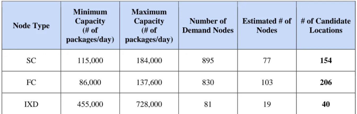
Using Coupa’s Supply Chain Guru X (SCGX) software, the greenfield analysis tool generated the best placement of candidate locations coordinates that are aligned with the distance-based approach (Coupa, 2021). To optimize for the best facility locations, the model requires enough candidate locations to draw from. Therefore, the number of candidate locations need to double the estimated number of nodes required for each type of location. Fortunately, the program’s map visualization tools help ensure the facilities generated are located close to main roads and not at unreachable locations. The following sections on candidate locations gather the input details on each type of the facilities and the distance-based approach formulation.

3.2.1 Inbound Cross-Dock (IXD) Candidate Locations

The IXD candidate locations can be solved by using the basic FLP distance-based approach. This approach locates the optimal location of multiple nodes by minimizing the average weighted distance from the demand. The demand locations in this case are the current major ports in the U.S. as well as the top locations of domestic sellers that currently sell to the sponsoring company. The number of demand for these locations is the aggregated volume processed at these ports and the percent of total domestic sellers’ volumes per location.

The mathematical formulation to solve for the IXD candidate locations is closely follow Watson et al.,’s (2012) formulation as follows:

𝑀𝑖𝑛. ∑ ∑ 𝑑_𝑥𝑎𝐷_𝑎𝑌_𝑥𝑎

𝑎 𝑥

(28)

28

This formula is subject to a number of constraints such as constraint (2) which make sure that every customer is fulfilled.

∑ 𝑌_𝑥𝑎 = 1

𝑥

∀𝑎 (2)

Constraint (3) is used to generate the number of candidate locations L in the network using the values that have been calculated before.

∑ 𝑋_𝑥

𝑥

= 𝐿 (3)

Constraint (4) ensures that a facility must process between its minimum and maximum capacities.

𝑈_{𝑥 𝑚𝑖𝑛} 𝑋_𝑥≤ ∑ 𝐷_𝑥𝑎𝑌_𝑥𝑎≤ 𝑈_{𝑥 𝑚𝑎𝑥} 𝑋_𝑥

𝑎

∀𝑥 ₍₄₎

The shipment between the two nodes cannot be made unless the facility is opened as reflected in constraint (5)

𝑌𝑥𝑎 ≤ 𝑋𝑥 ∀𝑥 ∀𝑎 (5)

Constraint (6) is a binary linking whether a lane is created between the candidate locations and its input.

𝑌_𝑥𝑎 ∈ {0,1} (6)

Constraint (7) is a binary linking whether to open the facility or not.

𝑋𝑥∈ {0,1} (7)

3.2.2 Fulfillment Center (FC) Candidate Locations

The FC candidate locations can be solved by also utilizing the distance-based approach. The demand locations in this case, however, will be based on 830 cities across the U.S. with populations above 50,000 residents. This method is used in order to avoid the tendencies of having FC closer towards the IXD candidate locations due to the distance-based approach.

Similarly, the mathematical formulation to solve for the FC candidate locations is closely follow Watson et al.’s (2012) formulation as follows:

𝑀𝑖𝑛. ∑ ∑ 𝑑𝑓𝑏𝐷𝑏𝑌𝑓𝑏 𝑏

𝑓

(29)

29

∑ 𝑌𝑓𝑏 = 1 𝑓

∀𝑏 (9)

∑ 𝑋𝑓 = 𝐿 𝑓

(10)

𝑈𝑓 𝑚𝑖𝑛 𝑋𝑓 ≤ ∑ 𝐷𝑓𝑏𝑌𝑓𝑏 ≤ 𝑈𝑓 𝑚𝑎𝑥 𝑋𝑓 ∀𝑓 𝑏

(11)

𝑌_𝑓𝑏 ≤ 𝑋_𝑓𝑏 ∀𝑓 ∀𝑏 (12) Constraint (13) is a binary linking whether a lane is created between the candidate locations and its input.

𝑌𝑓𝑏 ∈ {0,1} (13)

𝑋_𝑓 ∈ {0,1} (14)

3.2.3 Sorting Center (SC) Candidate Locations

The sorting center candidate location can also be solved by using the same approach taken to locate IXD and FC candidate locations. The customer demand input in this case is provided as a U.S. 3-digit ZIP code format, aggregating demand by sectional divides within each state. This method selects candidate locations closer to zip codes with higher demands.

The minimum capacity requirements will limit the number of SC candidate locations, aggregating demand in certain ZIP-codes to be served by fewer SC. Maximum capacity limitations, however, may increase the number of candidate locations necessary to meet certain zip-codes’ demand.

Similarly, the mathematical formulation to solve for the SC candidate locations is closely follow Watson et al.’s (2012) formulation as follows:

(30)

30

𝑀𝑖𝑛. ∑ ∑ 𝑑_𝑠𝑐𝐷_𝑐𝑌_𝑠𝑐

𝑐 𝑠

(15)

∑ 𝑌_𝑠𝑐= 1

𝑠

∀𝑐 ₍₁₆₎

∑ 𝑋_𝑠 = 𝐿

𝑠

(17)

𝑈𝑠 𝑚𝑖𝑛 𝑋𝑠 ≤ ∑ 𝐷𝑠𝑐𝑌𝑠𝑐 ≤ 𝑈𝑠 𝑚𝑎𝑥 𝑋𝑠 𝑐

∀𝑠 ₍₁₈₎

𝑌_𝑠𝑐 ≤ 𝑋_𝑠𝑐 ∀𝑠 ∀𝑐 (19) Constraint (20) is a binary linking whether a lane is created between the candidate locations and its input.

𝑌𝑠𝑐∈ {0,1} (20)

𝑋𝑠∈ {0,1} (21)

3.2.4 Annotations and Mathematical Formulations

𝑎𝑖 : Public terminals or domestic supplier number i as Greenfield input for

IXD

𝑏𝑗 : Cities above 50,000 population number j as Greenfield input for FC

𝑐𝑘 : Customer demand number k as Greenfield input for SC

𝑥_𝑖 : Inbound Cross-Docks (IXD) number i 𝑓_𝑗 : Fulfillment Center (FC) number j 𝑠_𝑘 : Sorting Center (SC) number k

(31)

31

𝐷_𝑎, 𝐷_𝑏, 𝐷_𝑐 : Facility supply capacity, number of populations, or customer demand for Greenfield input

𝐷_𝑥𝑎, 𝐷_𝑓𝑏, 𝐷_𝑠𝑐 : Supply capacity assigned to IXD, number of populations assigned to FC, or customer demand assigned to SC

𝑑𝑥𝑎, 𝑑𝑓𝑏, 𝑑𝑠𝑐 : Distance of travel between candidate locations and its Greenfield input

(public terminals and domestic suppliers, cities above 50,000 population, or customer demand

𝑈_𝑥, 𝑈_𝑓, 𝑈_𝑠 : Capacity of each facility

𝑌_𝑥𝑎,𝑌_𝑓𝑏,𝑌_𝑠𝑐 : Binary linking, 1 if candidate locations x/f/s serve the Greenfield input a/b/c

𝑋_𝑥, 𝑋_𝑓, 𝑋_𝑠 : Binary linking, 1 if candidate locations x/f/s are opened

L : Number of candidate locations for each facility to be generated (IXD = 30, FC = 206, SC = 154)

Locating facilities using the distance-based approach can be generalized as the following objectives and constraints where xa indicates a pairing for IXD and it’s Greenfield input from public terminals or domestic suppliers information. Use fb annotation pairing to find candidate locations for FC and sc annotation pairing to find candidate locations for SC.

𝑀𝑖𝑛. ∑ ∑ 𝑑_𝑥𝑎𝐷_𝑎𝑌_𝑥𝑎 𝑎 𝑥 (1) s.t. ∑ 𝑌_𝑥𝑎 = 1 𝑥 ∀𝑎 ₍₂₎ ∑ 𝑋_𝑥 𝑥 = 𝐿 ₍₃₎ 𝑈_{𝑥 𝑚𝑖𝑛} 𝑋_𝑥≤ ∑ 𝐷_𝑥𝑎𝑌_𝑥𝑎≤ 𝑈_{𝑥 𝑚𝑎𝑥} 𝑋_𝑥 𝑎 ∀𝑥 ₍₄₎ 𝑌_𝑥𝑎 ≤ 𝑋_𝑥 ∀𝑥 ∀𝑎 (5) 𝑌_𝑥𝑎 ∈ {0,1} (6) 𝑋𝑥∈ {0,1} (7)

3.3 Formulating Objectives

Once candidate locations for IXD, FC, and SC are identified as a fixed set of number of facilities, the network optimization model is then categorized as a discrete model. Discrete

(32)

32

models mean that the number of nodes is restricted to a finite number of locations (Daskin, 2008). Additionally, one of the key variables that build-up to each objective is the distance between the nodes. Thus, under the umbrella of discrete models, optimizing the distance between nodes in this model is categorized as a p-median discrete model (Daskin, 2008). This constraint applies to the GFLP optimization to achieve the three objectives in minimizing carbon emission, transportation cost, and delivery time.

3.3.1 Carbon Emissions

The first objective function is to minimize total carbon emissions of the network. The model utilizes the GLEC Framework to account for carbon emissions. Per the GHG Protocol and GLEC Framework, all the emissions in scope for this research, the transportation emissions required to move goods, is calculated using the method for Scope 3 emissions. As explained in Section 2.2, Scope 3 is used to estimate transportation emissions in the supply chain when the actual fuel burn data is unavailable, and when the split between company-owned vs. subcontracted transportation is unknown.

To accurately calculate carbon emissions from transportation, the GLEC Framework includes the full fuel life cycle, also known as the well-to-wheel (WTW) carbon intensity factors (Greene and Lewis, 2019). The WTW emissions is the sum of both the fuel emissions from well-to-tank (fuel production and distribution) and from tank-to-wheel (fuel combustion). Carbon intensity factors were selected from the GLEC Framework that most closely align with the transportation vehicles and activities used in this study. For electric-powered vehicles, electricity use is converted to carbon emissions by accounting for the sources of energy used to create electricity, expressing its emissions factors in mass carbon emissions (CO2e) per kilowatt-hours (kWh) of electricity used.

Scope 3 emissions are calculated based on the following formula:

𝑘𝑔 𝐶𝑂₂𝑒 𝑒𝑚𝑖𝑠𝑠𝑖𝑜𝑛𝑠 = ∑ 𝑡𝑜𝑡𝑎𝑙 𝑡 ∗ 𝑘𝑚 ∗ 𝐶𝑂₂𝑒 𝑖𝑛𝑡𝑒𝑛𝑠𝑖𝑡𝑦 𝑓𝑎𝑐𝑡𝑜𝑟 (23)

Thus, total emissions per trip can be calculated following the below steps:

1. Calculate total tonne-kilometer(tkm) by estimating total weight (t) per trip per transportation type and the total distance (km) traveled by the same transportation type between nodes

2. Determine carbon intensity factor(s) of transportation types (CO2e intensity factor) 3. Convert tonne-kilometer to CO2e emissions per transportation type

(total tkm * CO2e intensity factor)

The average weight per shipment is pre-determined for each vehicle type per MMTN’s requirements. Distance between nodes will be derived from the optimization of the model

Carbon Efficient Network Design: Evaluating The Trade-Offs Between Carbon Emissions, Transportation Cost and Delivery Time For a Middle-Mile Distribution Network

Carbon Efficient Network Design:

Evaluating the Trade-Offs Between Carbon Emissions, Transportation Cost,

and Delivery Time for a Middle-Mile Distribution Network

Carbon Efficient Network Design:

Evaluating the Trade-Offs Between Carbon Emissions, Transportation Cost,

and Delivery Time for a Middle-Mile Distribution Network

ACKNOWLEDGEMENTS

TABLE OF CONTENTS

LIST OF FIGURES

LIST OF TABLES

1. Introduction

1.1 Motivation for the Study

1.2 Research Questions

1.3 Approach

2. Literature Review

2.1 Network Design

2.2 Measuring Carbon Emissions in Supply Chains

2.3 Emerging and Existing Carbon Efficient Transportation Modes

2.4 Business Impact of Carbon Efficient Network Design

2.5 Summary

3. Data and Methodology

3.1 Assumptions

3.2 Candidate Locations

3.3 Formulating Objectives