View of Acceleration
in First Order Optimization
by
Jingzhao Zhang
B.S., University of California, Berkeley(2016)
Submitted to the Department of Electrical Engineering and
MIASSACHUSETTS INSTITUTE OFTECHNLOGY
JUN 13 2019
LIBRARIES
ARCHIVES
Computer
Science
in partial fulfillment of the requirements for the degree of
Master of Science
at the
MASSACHUSETTS INSTITUTE OF TECHNOLOGY
June 2019
®
Massachusetts Institute of Technology 2019.
A uthor ...
All rights reserved.
Signature redacted
Department of Electrical Engineering and Computer Science
Certified by...
Signature redacted
May 10, 2019
Suvrit Sra
Associate Professor of Electrical Engineering and Computer Science
Certified by
Signature redacted
Thesis Supervisor
Ali Jadbabaie
JR East Professor of Engineering
Department of Civil and Environmental Engineering
Institute for Data, Systems and Society
Accepted by
...
.Signature
redacted
Thesis Supervisor
t- -
Leslie A. Kolodziejski
Professor of Electrical Engineering and Computer Science
Chair, Department Committee on Graduate Students
Dynamical Systems View of Acceleration
in First Order Optimization
by
Jingzhao Zhang
Submitted to the Department of Electrical Engineering and Computer Science on May 10, 2019, in partial fulfillment of the
requirements for the degree of Master of Science
Abstract
Gradient based optimization algorithms are among the most fundamental algorithms in optimization and machine learning, yet they suffer from slow convergence. Conse-quently, accelerating gradient based methods have become an important recent topic of study. In this thesis, we focus on explaining and understanding the acceleration results. In particular, we aim to provide insights into the acceleration phenomenon and further develop new algorithms based on this interpretation. To do so, we follow the line of work on the continuous ordinary differential equation representations of momentum based acceleration methods. We start by proving that acceleration can be achieved by stable discretization of ODEs using standard Runge-Kutta integrators when the function is smooth enough and convex. We then extend this idea and de-velop a distributed algorithm for solving convex finite sum problems over networks. Our proposed algorithm achieves acceleration without resorting to Nesterov's momen-tum approach. Finally we generalize the result to functions that are quasi-strongly convex but not necessarily convex. We show that acceleration can be achieved in a nontrivial neighborhood of the optimal solution. In particular, the neighborhood can grow larger as the condition number of the function increases. The results altogether provide a systematic way to prove nonasymptotic convergence rates of algorithms derived from ODE discretization.
Thesis Supervisor: Suvrit Sra
Title: Associate Professor of Electrical Engineering and Computer Science Thesis Supervisor: Ali Jadbabaie
Title: JR East Professor of Engineering
Department of Civil and Environmental Engineering Institute for Data, Systems and Society
Acknowledgments
First and foremost, I want to thank my advisors, Suvrit and Ali, for their guidance in the past two years. This work cannot be completed without their incredibly insightful help. I would also like to thank my collaborators and everyone in our research group.
I have very much benefited from their informative presentations and sharp academic
discussions.
I wish to thank my family, especially my parents for their unconditional support of my decisions. I am deeply indebted to my parents for not accompanying them more in the past six years. I wish to thank my friends for giving me their honest advice ranging from mathematics to cooking, for always being there to hear my complaints and to share my emotions either in person or through wechat. Lastly, I wish to thank the Charles River for its endurant presence and for its beauty throughout the year except for the winter that lasted five months.
Contents
1 Motivations and Outline 13
2 Introduction 15
2.1 A brief overview of convex optimization . . . . 15
2.2 First order optimization algorithms . . . . 17
2.3 Accelerated gradient descent . . . . 18
2.3.1 Understanding acceleration . . . . 22
2.4 ODE interpretation of Nesterov's method . . . . 23
2.4.1 More related work on ODE interpretations . . . . 25
2.5 Main contributions of the thesis . . . . 25
3 Achieving Acceleration via Discretization 27 3.1 Numerical integration . . . . 27
3.1.1 Runge-Kutta integrators . . . . 28
3.2 Smooth convex problems . . . . 29
3.2.1 Problem setup . . . . 29
3.2.2 M ain result . . . . 31
3.2.3 Proof of Theorem 3.2.1 . . . . 35
3.2.4 Numerical experiments . . . . 38
3.2.5 Technical lemmas of the proof . . . . 42
4 Extensions of Acceleration via ODE Discretization 67 4.1 An application to distributed optimization . . . . 67
4.1.1 Problem formulation . . . . 67
4.1.2 Dual dom ain raepresentation . . . . 69
4.1.3 Algorithm . . . . 72
4.1.4 Convergence analysis . . . . 75
4.2 Quasi-strongly convex problems . . . . 76
4.2.1 Algorithm . . . . 78
4.2.2 Convergence analysis . . . . 79
4.2.3 Numerical experiments . . . . 81
4.2.4 Discussion . . . . 82
List of Figures
3-1 Convergence paths of GD, NAG, and the proposed simulated dynam-ical system with integrators of degree s = 1, s = 2, and s = 4. The
objectives satisfy Assumption 3.2.1 with p=2. . . . . 40
3-2 Minimizing quadratic objective by simulating different ODEs with the RK44 integrator (4th order). In the case when p = 2, the optimal
choice for q is 2. . . . . 41
3-3 Experiment results for the cases that Assumption 3.2.1 holds for p > 2. 41
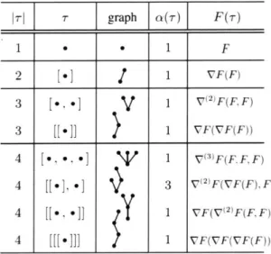
3-4 A figure adapted from Hairer et al. [2006]. Example tree structures and corresponding function derivatives. . . . . 65
4-1 Convergence paths for GD, NAG and direct discretization algorithms. The objective is quadratic and described in (4.25). . . . . 82
4-2 Convergence paths for GD, NAG and direct discretization algorithms. The objective is a logistic regression loss described in (4.26). .... 82
List of Tables
2.1 Iteration complexities of GD and NAG with and without strong con-vexity. . . . . 22 4.1 Iteration complexity of centralized and decentralized approaches for
Chapter 1
Motivations and Outline
Gradient based optimization algorithms have attracted increasing attention as neural network training methods have become more powerful and popular. Consequently, much efforts have been made to accelerate the convergence of first order optimization both from theoretical and empirical perspectives. From the theory side, many new algorithms were proven to accelerate upon gradient descent under both deterministic and stochastic settings. These algorithms utilize beautiful ideas such as variance reduction, Nesterov's acceleration, restart, and local regularization. The convergence criteria studied involve function suboptimality, first-order stationarity and second-order stationarity. In addition, a sequence of work also constructs examples to provide theoretical lower bounds for gradient based algorithms.
However, it has been observed that theoretically accelerated algorithms do not always yield good empirical performance. As a result, many techniques have been proposed with a focus on experimental convergence rates. Examples include batch normalization, heavy-ball style momentum and adaptive step sizes. Though these techniques are based on high level motivations, formal proofs of acceleration are in general missing. This gap leads to research in providing theoretical insights into these techniques in the hope that more algorithms and structures can be discovered in this process.
Given the wide range of applications and the large number of open questions in this area, research in accelerating gradient based optimization algorithms is both
challenging and important. In this thesis, we contribute to this topic by focusing on explaining the acceleration phenomenon of Nesterov's momentum method. Based on this explanation, we design a family of provably accelerated algorithms. Particularly, the thesis is organized as follows.
In Chapter 2, we provide a brief introduction to convex optimization. We define a few key concepts required to formally quantify acceleration. We analyze gradient descent as a starting point and then present theories developed by Nesterov and Ne-mirovsky on accelerated gradient descent. In this process, we appreciate its elegance but also understand why this technique requires further understanding.
In Chapter 3, we focus on an ordinary differential equation (ODE) based per-spective for understanding Nesterov's momentum approach. We prove that based on this idea, we can achieve acceleration by simply discretizing a family of second order ODEs with standard integration methods from numerical analysis. Algorithms designed this way are conceptually simple and can even achieve convergence faster than Nesterov's accelerated gradient descent when the objectives satisfy additional flatness assumptions.
In Chapter 4, we demonstrate that the discretization technique studied above can be generalized to solve more problems such as distributed optimization and quasi-strongly convex optimization. Lastly, we discuss probable future work and conclude the thesis.
Chapter 2
Introduction
In this chapter, we explain the problem setup by going over some basic concepts in convex optimization. A large part of this chapter is based on the textbook [Nesterov,
2013].
2.1
A brief overview of convex optimization
We start by briefly reviewing the formulation of optimization problems. Let x be a vector in Rd. Let
f
: Rd -+ R be the objective function. We would like to choose x in order to solve the following minimization problem,min f(x) s.t. x
c
S, (2.1)where S C Rd denotes the feasible set and encodes problem constraints. This problem formulation covers a large number of applications in machine learning and operation research but is in general intractable. As this thesis focuses on analyzing the time complexity of polynomial time algorithms, we introduce the concept of convexity in order to help make the problem tractable.
Definition 2.1.1. A set S E Rd is convex if for all x, y c S, A E [0,1],
The definition can be interpreted in a geometrical way that the line segment between any two points of S is contained in S. Based on this notion, we can define the convexity of a real valued function.
Definition 2.1.2. A function
f
: X -+ R is convex if it has a convex epigraph,epi(f) = {(x, y) x E X, y > f (x)}.
For simplicity, we assume throughout this thesis that there is a global minimum
x*. When
f
is differentiable and convex, we know that x* is optimal if and only ifVf (x*) = 0. Convexity also leads to a few equivalent definitions if f(x) is continuously
differentiable. Please see [Nesterov, 2013] for proofs.
Lemma 2.1.1. A function f is convex and continuously differentiable if and only if
for all x, y in Rd, and a in [0, 1) one of the following holds,
1. f (y) > f (x) + (Vf (x), y - x),
2. f (ax + (1 - a)y) < af(x) + (1 - af (y),
3. (Vf (x) - Vf (y), x - y) > 0.
Based on the above definition, we can define p-strong convexity to quantify the strength of convexity.
Definition 2.1.3. A continuously differentiable function
f
is p-strongly convex if for all x, y E Rd,f(y) f (x) + (Vf (x), y - x) + P 2 x - y112
To further ease our analysis, we very often bound the variation of the function
f
by bounding the Lipschitz constant of its gradient.
Definition 2.1.4. A differentiable function f(x) is L-smooth if for all x, y in Rd,
The concept of acceleration will be critically built on the definitions above. Algorithms for convex optimization evolved very fast during the last century. Many ground-breaking algorithms such as ellipsoid methods, interior point methods, quasi-newton methods were developed. The time and space complexities of these algorithms usually grows super linearly in the number of variables d. In this thesis, we focus on first order optimization algorithms that usually have linear dependency on the problem dimension d.
2.2
First order optimization algorithms
Throughout this thesis, we will study the iteration complexity (will be defined) of deterministic first order optimization algorithms. In particular, each iteration involves one oracle call that takes in a point x and returns the function value and the gradient evaluated at x, (f(x), Vf(x)). An iterative algorithm generates a sequence of points
{Xk}k>o
based on the feedback from oracle calls. Following [Nesterov, 20131, we constrain ourselves to iterative algorithms satisfyingXk E xo + Lin{Vf (Xo), ... , Vf (Xk-1)}, for k > 1, (2.2)
where Lin denotes the linear span. We denote an algorithm by A -which is determined
by the mappings Ak from previous oracle calls to the next point in the sequence, i.e.
Xk+1 - Ak (Xo, Vf (Xo), ..., Xk, Vf (xk)).
Now we are ready to define iteration complexity. Denote by A[f, xoj the sequence of points {Xk} generated by algorithm A with function
f
starting from xo. Let-Then the complexity of algorithm A on function class F is defined as
T(A, F) = sup T (A[f, ol, f)
f ET
To provide a concrete example, we take a close look at the gradient descent algo-rithm. Let T,,L denote the class of functions that are differentiable, L-smooth and p--strongly convex. Consider the following gradient descent update,
1
Xk+1 = Xk - --Vf(x). (2.3)
L
Then by smoothness and strong convexity (see Thm 2.1.15 in Nesterov 12013] for details), one can show that
f(xk) -
f*
< - O -- x*H2.2 p+ L
Therefore, the iteration complexity of gradient descent (2.3) for minimizing functions
in F,,L is of order O(L log(Ljxo-x*j-)).
2.3
Accelerated gradient descent
As discussed in Section 2.2, we know that gradient descent (GD) has iteration com-plexity O(L log(')). However, [Nemirovskii and Yudin, 1983] proves a lower bound on iteration complexity of O( log(-)). Soon Nesterov answered this question in Nesterov
[19831
by proposing an accelerated algorithm now known as Nesterov'sac-celerated gradient descent (NAG). In this subsection, we go over the result including its proof to show its mysteriousness and elegance. This result motivates a line of work trying to explain and understand the acceleration phenomenon.
We first present the heavy-ball algorithm proposed in [Polyak, 1964]. Recall that
GD can be written as
Polyak modified the update by including a momentum term such that the update looks like the following,
Xk 1 =Xk - aVf (Xk) + /3(Xk - Xkl1). (2.4)
This algorithm is now known as gradient descent with momentum or the heavy-ball method. In Polyak's original work, he proved that when the objective is quadratic, L-smooth and p-strongly convex, with properly chosen a and /, the algorithm 2.4 has iteration complexity O( log(!)). Notice that this is significantly faster than
GD when L/p is large. The quantity is also called the condition number,
L
Q=.
Polyak [1964] showed the possibility of accelerating gradient descent with momen-tum for strongly convex quadratic objective functions. However, the proof critically relies on the quadratic assumption. Whether this algorithm leads to acceleration in the general smooth strongly convex setting is still an open problem.
Later, Nesterov [19831 proposed the following algorithm to close the gap.
Yk+1 = Xk - aVf(xk) (2.5)
Xk+1 = (1 + )yk+1 - /3
Yk-This is the famous Nesterov's accelerated gradient descent algorithm and is similar to the heavy ball algorithm except that the gradient is evaluated at an interpolated point between two adjacent iterates. With this algorithm, Nesterov proved the following result.
Theorem 2.3.1. Let f be p-strongly convex and L-smooth, then NAG defined in (2.5) with parameter choice a = =
2,
satisfiesThis implies that the iteration complexity of NAG for p-strongly convex, L-smooth
functions is O( :log(,)).
Proof. A large portion of the proof follows the very clear and instructive blog post1 .
The core idea is the same as Nesterov's original technique known as the estimated sequence.
We define a sequence of p--strongly convex functions ?k (x), k > 0 as
1o(x) = f(xo) + P||x -
xo0
2,
2
4Dk 1(X) =(1 - I %>Ik(x) + (f (xk) + KVf (xk), X - Xk) + 11jx - x k 112).
One can easily prove by induction that @k(x) is a lower bound for f(x) in the following sense
k(x) < f(X) + (1- )'((W - f ).
By Lemma 2.3.2, we then obtain the upper-bound,
f(Yk) min k(x).
xBRd
Based on this bound, we can conclude that
f(Yk) - f(x*) Ok(X) - f(x*) <
< p -~2 LX2 - X* 12(
(1- )k( o(x*) - f(x*))
1
k-1
which completes the proof F
Below we prove the lemma above and complete the entire proof.
'blogs. princeton. edu/ imabandit/ 2014 /03 /06 /nesterovs-accelerated-gradient-descent-for-smooth-and-strongly-convex-optimization/
Lemma 2.3.2. In the context of Theorem 3.2.1, we have
f (Yk) < min 4k (x). PERd
Proof. Denote b* = min~saGyx)
f(yk+1) <- f(Xk) - 11'f(Xk 12 = (1 -)f (yk) + (1 -) 1 )*+ 17 /(1 -Q- )k* + (1 - )( 1 1 (f(xk) - f(Yk)) + f(xk) - -1Vf(k)1 2
Q
2L f (Xk), Xk - Yk) + f (X)- 11'f (Xk) 12What remains to show is that
1 - )(Vf (x),xk - yk) 1 + f
(Xk)-IQ
1L
Vf (Xk) < -2 +-(2.6)Note that <Dk(X) is quadratic and can be written as
)k(X) = k P
--Vk11 2 2
where Vk+1 (1 - $)Vk x - Vf(xk) (derived by taking derivative to be
0). Now by evaluating ok+1(x) at Xk, we get the following
D+* =(1- )* +
f
(x) + 2 (1)Xk - Vk112
11 1
2 (Xk) 2 +f
-(-
Q
Q
(7f rX), Vk -Xk).Comparing against (2.6), we only need to show that Vk - Xk = Q(xk - Yk) This
is done via induction and applying the update iteration.
Now that we have gone through the proof for analyzing the convergence rate of
NAG when the function is smooth and strongly convex. The proof shows that NAG
Gradient descent Nesterov's method Lower bound
Smooth & Convex _ _y) _O(
)
O( )
Smooth & strongly convex O(L log( )) ( log( )) O( L log( )) Table 2.1: Iteration complexities of GD and NAG with and without strong convexity.
accelerates GD by improving the dependency on A to . Even though the proof is elegant and elementary, it is unclear how one could come up with it in the first place. The main goal of this thesis is to provide more intuitions into this method and propose an alternative way to achieve acceleration.
Before moving on to the discussion of understanding NAG, a few more comments are in order. First, up to now, we have only discussed the proof for GD and NAG under the strong convexity assumption. There is a counterpart for acceleration when the function is convex but not necessarily strongly convex. In fact, it is folklore knowledge that accelerated methods for strongly convex function can be used to accelerate smooth convex problems by regularization. On the other hand, accelerated methods for smooth convex problems can accelerate strongly convex problems by restart.
Furthermore, Nemirovskii and Yudin
[19831
shows that the accelerated methods proposed in[Nesterov,
1983] is up to a constant optimal. In other words, any firstorder algorithm satisfying (2.2) can not have an iteration complexity that is more than a constant better than NAG. The lower bound is established via constructing a quadratic function whose gradients has zeros in most coordinates. For details of the proof, please refer to [Nesterov, 2013, Chapter 2]. The key results are summarized in Table 2.1.
2.3.1
Understanding acceleration
The theory of acceleration in convex optimization is complete in the sense that the gap between the upper and lower bound is closed. However, ever since its introduc-tion, acceleration has remained somewhat mysterious, especially because of Nesterov's
original derivation relies on elegant but unintuitive algebraic arguments. This lack of understanding has spurred a variety of recent attempts to uncover the rationale behind the phenomenon of acceleration.
Allen-Zhu and Orecchia [20141 consider NAG as a linear coupling between mirror descent2 and gradient descent. Bubeck et al. [2015] propose a geometric interpretation
of acceleration that considers an iterative process as shrinking the radius of a ball which covers the optimal solution. Acceleration can be then achieved by choosing the radius carefully. Lessard et al. [2016], Hu and Lessard 12017] study acceleration from a control theoretic perspective. They formulate the optimization algorithm as a controller to a nonlinear dynamical system. The convergence rate can be solved numerically using an SDP with integral quadratic constraints. Scieur et al. [2016] achieve acceleration via averaging past iterates. The weights are derived by solving a linear system inspired by Chebyshev polynomials.
Aside from above, there is a large body of literature that studies acceleration from a continuous time perspective. As our thesis follows this line of research, we explain this idea in details below.
2.4
ODE
interpretation of Nesterov's method
In this section, we will elaborate on understanding acceleration from an ordinary differential equation(ODE) perspective. Most of the content is extracted from [Su et al., 2014]. In particular, we focus on the NAG algorithm for optimizing smooth convex functions, i.e.
Xk = Yk-1 - hVf(yk_1), (2.7)
y = Xk +k 1 (x -xk-1), k + 1
where the standard choice of the parameter is h = . Notice that this is different from the expression in (2.5). Particularly, the coefficient 3 becomes iteration dependent
2
An algorithm that generalizes gradient descent by using Bregman divergence instead of Euclidean distance.
due to lack of strong convexity. We can rewrite the expression (2.7) and obtain,
Xk+1 - Xk _ k - 1 Xk - Xkl-1 VV f (Yk).
V~h__ k +2 V/7_
If we let X(t) be a smooth curve and X(kVh) ~ x k, then based on the above equation
we can send the step size h - 0 and obtain the following ODE:
3
X+ -X +Vf(X) = 0.
t (2.8)
This ODE is the continuous analog of the original NAG algorithm (2.7) in the fol-lowing sense,
Theorem 2.4.1 (Su et al. [20141). For any smooth convex function
f
and x0 E Rd,the ODE (2.8) with initial conditions X(0) = x0 and X(0) = 0 has a unique global
solution X(t) that is twice continuously differentiable from (0, oc) to Rd. Furthermore, for all fixed T > 0,
lim max ||xk - X(kh)|| = 0. h-+O <k<T
The above theorem states that as the step size h goes to generated by NAG will converge to the trajectory defined
(2.8).
Furthermore, we know that the function suboptimality
at the rate !. This property is preserved by its continuous
0, the sequence of points
as the ODE solution to
f(xk)
- f(x*) convergeslimit in the sense that
f (X(0)) - f(x*) < 2|xo x* 2 (2.9)
The proof of 2.9 relies on defining the Lyapunov function:
4(t) = t2(f(X(t)) - f(x*))
+ 2 |X + tk/2 - x*| 2
conceptually simple and turns out to be critical in proving the theorems stated in the next chapter.
2.4.1
More related work on ODE interpretations
The ODE interpretation of optimization algorithms has a long history, and has been studied for example in [Alvarez, 2000, Attouch et al., 2000, Bruck Jr, 1975, Attouch and Cominetti, 1996]. These work analyzed the asymptotic behavior of solutions to dissipative dynamical systems. The more recent sequence of work on the ordinary
ODE interpretation of the acceleration took more interest in the non-asymptotic
analysis and discretized algorithms. Later, Wibisono et al. [2016], Xu et al. [2018], Krichene et al. [2015], Franga et al. [2018], Barakat and Bianchi [20181 generalized this idea to study the continuous limit of other first order algorithms such as mirror descent, ADMM, ADAM. Shi et al. [2019], Betancourt et al. [2018], Shi et al. [2018] studied the discretization of ODE and aim to design accelerated algorithms, but the discretization either does not have theoretical guarantee or requires prior knowledge of Nesterov's method.
2.5
Main contributions of the thesis
Although previous works on ODE interpretations of accelerated methods succeed in providing a richer understanding of Nesterov's scheme via its continuous time ODE, they fail to provide a general discretization procedure that generates provably
con-vergent accelerated methods. In the rest of this thesis, we introduce a family of second-order ODEs that generate accelerated first-order methods if we simply dis-cretize them using any Runge-Kutta numerical integrator and choose a suitable step size.
The results will be based on three published works. Chapter 3 summarizes the work in [Zhang et al., 2018a]. We achieve acceleration by simply discretizing a family of second order ODEs for smooth convex functions. Algorithms designed this way are conceptually simple and can even achieve faster convergence than Nesterov's
acceler-ated gradient descent when the objectives satisfy additional flatness assumptions. In Chapter 4, we present the results in [Zhang et al., 2018b, 2019]. We demonstrate that the discretization technique above can be generalized to solve more problems such as distributed optimization and quasi-strongly convex optimization.
Chapter 3
Achieving Acceleration via
Discretization
In this chapter, we introduce a sequence of second-order ODEs that generate an accelerated first-order method for smooth functions if we simply discretize it using any Runge-Kutta numerical integrator and choose a suitable step size. Most of the content is based on our work in
[Zhang
et al., 2018a].3.1
Numerical integration
As it is not always possible to solve ODEs analytically, numerical integration methods are often used to simulate trajectories approximately. Particularly, we first rewrite ODEs as an autonomous dynamical system,
y
= F(y). (3.1)For example, we can rewrite the ODE in (2.8) as following:
, where y = [v;x; rT]. (3.2)
-AVo - Vf (X)
y=F(y)
=VNumerical integrators aim to solve for y(t) with fixed initial value y(O) = yo. The
simplest of all numerical methods is the explicit Euler Method,
yn+1 yn + hF(y.).
Then y(t) is approximated with YLt/hj. Under mild regularity conditions of F(y), the approximation error converges to 0 as h -+ 0. However, this result is asymptotic. The
major challenge we solve in this chapter is to quantify the convergence and achieve non-asymptotic results.
3.1.1
Runge-Kutta integrators
Let us briefly recall explicit Runge-Kutta (RK) integrators. For a more in depth discussion please see the textbook [Hairer et al., 2006].
Definition 3.1.1. Given a dynamical system
y
F(y), let the current point be yoand the step size be h. An explicit S stage Runge-Kutta method generates the next step via the following update:
gi = yo + h aiF(g), (3.3)
j=1
S
4Jh(Yo) - yo + h biF(gi),
where aij and bi are suitable coefficients defined by the integrator; (Dh(Yo) is the esti-mation of the state after time step h, while gi (for i = 1, . . ., S) are a few neighboring
points where the gradient information F(gi) is evaluated.
By combining the gradients at several evaluation points, the integrator can achieve higher precision by matching up Taylor expansion coefficients with respect to t. Let Ph(yo) be the true solution to the ODE with initial condition yo; we say that an
integrator (Dh(yo) has order s if its discretization error shrinks as
Here we list a few examples of Runge-Kutta integrators and describe their order. The explicit Euler's method defined by <h(Yo) yo
+
hF(yo) is an explicit RK method oforder 1, while the midpoint method <h (yo) yo+hF(yo+AF(yo)) is of order 2. Some
high-order RK methods are summarized in Verner [1996]. An order 4 RK method requires 4 stages, i.e., 4 gradient evaluations, while an order 9 method requires 16 stages.
3.2
Smooth convex problems
In this section, we summarize the result in [Zhang et al., 2018b] and prove that acceleration can be achieved by simply discretizing an ODE similar to (2.8).
3.2.1
Problem setup
We assume that the objective
f
is convex and sufficiently smooth(defined later in this section). Our result rests on two key assumptions introduced below. The first as-sumption is a local flatness condition onf
around a minimum; our second assumption requiresf
to have bounded higher order derivatives. These assumptions are sufficient to achieve acceleration simply by discretizing suitable ODEs without either resorting to reverse engineering to obtain discretizations or resorting to other more involved integration mechanisms.We will require our assumptions to hold on a suitable subset of Rd. Let xo be the initial point to our proposed iterative algorithm. First consider the sublevel set
S := {x E Rd I f (x) < exp(1)((f (xo) - f (x*) + ||xo - x*fl2) + 1}, (3.5)
where x* is the optimal solution. Later we will show that the sequence of iterates obtained upon discretizing a suitable ODE never escapes this sublevel set. Thus, the assumptions that we introduce need to hold only within a subset of Rd. Let this
subset be defined as
A := {x E Rd I 3X' E S, J|x - X'1l < 1}, (3.6)
that is, the set of points at unit distance to the initial sublevel set (3.5). The choice of unit distance is arbitrary, and one can scale that to any desired constant.
Below we introduce the flatness condition.
Assumption 3.2.1. There exists an integer p > 2 and a positive constant L such
that for any point x E A, and for all indices i E
{1,
... , p -1}, we have the lower-boundf(x) - f(x*) > I VI ff(x) (3.7)
where x* minimizes
f
and IIV f (x) denotes the operator norm of the tensor VN Wf(x).Assumption 3.2.1 bounds high order derivatives by function suboptimality, so that these derivatives vanish as the suboptimality converges to 0. Thus, it quantifies the flatness of the objective around a minimum. When p = 2, Assumption 3.2.1 is slightly
weaker than the usual Lipschitz-continuity of gradients (see Example 3.2.1) typically assumed in the analysis of first-order methods, including NAG. If we further know that the objective's Taylor expansion around an optimum does not have low order terms, p would be the degree of the first nonzero term.
Example 3.2.1. Let
f
be convex withy-Lipschitz
continuous gradients, i.e.,||Vf(x)-Vf(y)| 1
y4x
- yl. Then, for any x, y E Rd we have,f (x) > f (y) + (Vf (y), x -y) + 1,Vf (x) - Vf (y)12.
In particular, for y = x*, an optimum point, we have Vf(y) = 0, and thus we have
f(x)
- f(x*)-}1,Vf
(x) 12, which is nothing but inequality (3.7) for p = 2 and i = 1.Example 3.2.2. Consider the fp-norm regression problem: min, f(x) =
H|Ax
- blIP,for even integer p > 2. If there exists x* such that Ax* = b, then
f
satisfies inequalityNext, we introduce our second assumption that adds additional restrictions on differentiability and bounds the growth of derivatives.
Assumption 3.2.2. There exists an integer s > p and a constant M > 0, such that
f(x) is order (s + 2) differentiable. Furthermore, for any x C A, the following operator
norm bounds hold:
|VJ7f(x) < M, for i =p,p+1, ... , s, s + 1, s + 2. (3.8)
When the sublevel sets of
f
are compact, the set A is also compact; as a result, the bound (3.8) on high order derivatives is implied by continuity. In addition, an Lploss of the form ||Ax - bJJP also satisfy (3.8) with M = p! |A J.
3.2.2
Main result
In this section, we introduce a second-order ODE and use explicit RK integrators to generate iterates that converge to the optimal solution at a rate faster than O(1/t) (where t denotes the time variable in the ODE). A central outcome of our result is that, at least for objective functions that are smooth enough, it is not the integrator type that is the key ingredient of acceleration, but a careful analysis of the dynamics with a more precise Lyapunov function that achieves the desired result. More specifically, we will show that by carefully exploiting boundedness of higher order derivatives, we can achieve both stability and acceleration at the same time.
We start by recalling Nesterov's accelerated gradient (NAG) method that is de-fined according to the updates
Xk = Yk-1 - hVf(yk_1), Yk Xk + [ti (Xk - Xkl)
ODE
z(t) + (t) + Vf (x(t)) 0, where = dx (3.9)
when one drives the step size h to zero. It can be further shown that in the
con-tinuous domain the function value f(x(t)) decreases at the rate of ((1/t 2) along the
trajectories of the ODE. This convergence rate can be accelerated to an arbitrary rate in continuous time via time dilation as in [Wibisono et al., 2016]. In particular, the solution to
s(t) + t-i(t) + p2tp-2Vf (x(t)) = 0, (3.10)
has a convergence rate O(1/tP). When p > 2, Wibisono et al. [2016] proposed rate matching algorithms via utilizing higher order derivatives (e.g., Hessians). In this work, we focus purely on first-order methods and study the stability of discretizing the ODE directly when p > 2.
Though deriving the ODE from the algorithm is solved, deriving the update of
NAG or any other accelerated method by directly discretizing an ODE is not. As
stated in [Wibisono et al., 2016], explicit Euler discretization of the ODE in (3.9) may not lead to a stable algorithm. Recently, Betancourt et al. [2018] observed empirically that Verlet integration is stable and suggested that the stability relates to the sym-plectic property of the Verlet integration. However, in our proof, we found that the
order condition of Verlet integration would suffice to achieve acceleration.
Though symplectic integrators are known to preserve modified Hamiltonians for dy-namical systems, we weren't able to leverage this property for dissipative systems such as (3.11).
This principal point of departure from previous works underlies Algorithm 1, which minimizes the objective by discretizing the following ODE with an order-s integrator:
2p + 1.
Algorithm 1: Input(f, xo, p, L, M, s, N) > Constants p, L, M are the same as in
Assumptions
1: Set the initial state yo = [0; xo; 1] - R2+I
2: Set step size h = C/Ni > C is determined by p, L, M, s, o
3: XN -- Order-s-Runge-Kutta-Integrator(F, yo, N, h) > F is defined in equation
3.12
4: return
XN-where we have augmented the state with time, to turn the non-autonomous dynamical system into an autonomous one. The solution to (3.11) exists and is unique when t > 0. This claim follows by local Lipschitzness of
f
and is discussed in more details in Appendix A.2 of Wibisono et al. [2016].We note that the ODE in (3.11) can also be written as the dynamical system
-- + -V - P 2tp-27 f(X)
F(y)
[
v
i
, where y = [v; x; t]. (3.12)L ~ 1
We have augmented the state with time to obtain an autonomous system, which can be readily solved numerically with a Runge-Kutta integrator as in Algorithm 1. To avoid singularity at t = 0, Algorithm 1 discretizes the ODE starting from t =1 with initial condition y(l) = yo = [0; xo; 1]. The choice of 1 can be replaced by any arbitrary positive constant.
Notice that the ODE in (3.11) is slightly different from the one in (3.10); it has a coefficient 2P+1 for t -(t) instead of Pl This modification is crucial for our analysis
t
via Lyapunov functions (more details in Section 3.2.3 and Appendix 3.2.5).
The parameter p in the ODE (3.11) is set to be the same as the constant in Assumption 3.2.1 to achieve the best theoretical upper bound by balancing stability and acceleration. Particularly, the larger p is, the faster the system evolves. Hence, the numerical integrator requires smaller step sizes to stabilize the process, but a smaller step size increases the number of iterations to achieve a target accuracy. This tension is alleviated by Assumption 3.2.1. The larger p is, the flatter the function
the iterates approach a minimum, the high order derivatives of the function f, in addition to the gradient, also converge to zero. Consequently, the trajectory slows down around the optimum and we can stably discretize the process with a large enough step size. This intuition ultimately translates into our main result.
Theorem 3.2.1. (Main Result) Consider the second-order ODE in (3.11). Suppose
that the function f is convex and Assumptions 3.2.1 and 3.2.2 are satisfied. Further, let s be the order of the Runge-Kutta integrator used in Algorithm 1, N be the total number of iterations, and x0 be the initial point. Also, let 8o := f(xo) - f(x*) +
|x0
- x*||2 + 1. Then, there exists a constant C1 such that if we set the step size ash = C1N-1/(s+1)(L+M+1)- , the iterate XN generated after running Algorithm 1
for N iterations satisfies the inequality
f(xN) - f(x*) 0280 [(L+M+ 0]P = o(N-P-r), (3.13)
where the constants C1 and C2 only depend on s, p, and the Runge-Kutta inte-grator. Since each iteration consumes S gradients, f(xN) - f(x*) will converge as
___ Ps
09(S + N- +) with respect to the number of gradient evaluations. Note that for com-monly used Runge-Kutta integrators, S < 8.
The proof of this theorem is quite involved; we provide a sketch in Section 3.2.3, deferring the detailed technical steps to the last subsection. We do not need to know the constant C1 exactly in order to set the step size h. Replacing C1 by any smaller
positive constant leads to the same polynomial rate.
Theorem 3.2.1 indicates that if the objective has bounded high order derivatives and satisfies the flatness condition in Assumption 3.2.1 with p > 0, then discretizing the ODE in (3.11) with a high order integrator results in an algorithm that converges to the optimal solution at a rate that is close to O(N-P). In the following corollaries, we highlight two special instances of Theorem 3.2.1.
Corollary 3.2.1. If the function f is convex with L-Lipschitz gradients and is 4th
integrator of order s = 2 for N iterations results in the suboptimality bound
C2(f(xo) -
f(x*)
+|xo - x*1'2 + 1)3(L + M + 1)2f(xN) - f~x)< N4/3
Note that higher order differentiability allows one to use a higher order integrator, which leads to the optimal O(N -2) rate in the limit. The next example is based on
high order polynomial or fp norm.
Corollary 3.2.2. Consider the objective function f(x) = flAx + b|14. Simulating the
ODE (3.11) for p = 4 with a numerical integrator of order s = 4 for N iterations results in the suboptimality bound
S<C2(f (X) -
f
(x*) + ||xo - x*K12 + 1)'(L + M + 1)4f(xN ) -- f(x) N16/5
3.2.3
Proof of Theorem 3.2.1
We prove Theorem 3.2.1 as follows. First (in Proposition 3.2.1), we show that the sub-optimality f (x(t))-f (x*) along the continuous trajectory of the ODE (3.11) converges to zero sufficiently fast. Second (in Proposition 3.2.2), we bound the discretization error I<bsh(yk) - Sh(yk) 1, which measures the distance between the point generated by
discretizing the ODE and the true continuous solution. Finally (in Proposition 3.2.3), a bound on this error along with continuity of the Lyapunov function (3.14) implies that the suboptimality of the discretized sequence of points also converges to zero quickly.
Central to our proof is the choice of a Lyapunov function used to quantify progress. We propose in particular the Lyapunov function S : R2
d+1 -+ R+ defined as t2 III2+t *1 f( )(-4 xV; X; t]) := 4 v||2 -- v - x* + t(f(x) - f (x*)). (3.14) 4p 2p
The Lyapunov function (3.14) is similar to the ones used by Wibisono et al. [2016], Su et al.
[20141,
except for the extra term 4,v2. This term allows us to boundLemma 3.2.5 for more details).
We begin our analysis with Proposition 3.2.1, which shows that the function 8 is non-increasing with time, i.e., 8(y) < 0. This monotonicity then implies that
both tP(f(x) - f(x*)) and
$2
v112 are bounded above by some constants. The boundon tP(f(x) - f(x*)) provides a convergence rate of 09(1/tP) on the sub-optimality
f(x(t)) -
f(x*).
It further leads to an upper-bound on the derivatives of the function f(x) in conjunction with Assumption 3.2.1.Proposition 3.2.1 (Monotonicity of 8). Consider the vector y = [v; x; t] E R+2d1 as
a trajectory of the dynamical system (3.12). Let the Lyapunov
function
8 be definedby (3.14). Then, for any trajectory y = [v; x; t], the time derivative $(y) is
non-positive and bounded above; more precisely,
8(y)
-- |v|2. (3.15)p
The proof of this proposition follows from convexity and (3.11); we defer the details to Appendix 3.2.5.
Next, to bound the Lyapunov function for numerical solutions, we need to bound the distance between points in the discretized and continuous trajectories. As in Section 3.1.1, for the dynamical system
Q
= F(y), let 4Dh(yo) denote the solutiongenerated by a numerical integrator starting at point yo with step size h. Similarly, let (Ph(Yo) be the corresponding true solution to the ODE. An ideal numerical integrator
would satisfy <Dh(Yo) = Ph(yo); however, due to discretization error there is always a
difference between <bh(yo) and Ph(yo), determined by the order of the integrator as in (3.4). Let {yf A be the sequence of points generated by the numerical integrator,
that is, yk+1 = 4'h(yk). In the following proposition, we derive an upper bound on
the resulting discretization error I<Dsh(yk) - .Ph(yk)I
Proposition 3.2.2 (Discretization error). Let yk = [vk; xk; tk] be the current state of
the dynamical system
p
= F(y) as defined in (4.11). Suppose Xk C S defined in (3.5).with a step size h such that h < min{0.2, (1+K)C(1+e(Y))(M+L+1)}' then
JCs+1 [(1 + 8(yk))]s+l h R1 + E(yk))]s+ 2
-|k<bh(yk)-po(yk)|| C'h+(M+L+l)
[
k+ tk,(3.16)1
tk tkwhere the constants C, ri, and C' only depend on p, s, and the integrator.
The proof of Proposition 3.2.2 is the most challenging part in proving Theo-rem 4.2.2. Details may be found in Appendix 3.2.5. The key step is to bound
11 s+ [4Dh(yk) - (Ph(yk)] |. To do so, we first bound the high order derivative tensor
|V(')f 1 using Assumption 3.2.1 and Proposition 3.2.1 within a region of radius R. By carefully selecting R, we can show that for a reasonably small step size h, <bh(yk)
and SPh(yk) are constrained in the region. Second, we need to compute the high order
derivatives of
y
= F(y) as a function of V()f which is bounded in the region ofradius R. As shown in Appendix 3.2.5, the expressions for higher derivatives become quite complicated as the order increases. We approach this complexity by using the notation for elementary differentials (see Appendix 3.2.5) adopted from Hairer et al.
[2006]; we then induct on the order of the derivatives to bound the higher order
derivatives. The flatness assumption (Assumption 3.2.1) provides bounds on the op-erator norm of high order derivatives relative to the objective function suboptimality,
and hence proves crucial in completing the inductive step.
By the conclusion in Proposition 3.2.2 and continuity of the Lyapunov function
E, we conclude that the value of E at a discretized point is close to its continuous counterpart. Using this observation, we expect that the Lyapunov function values for the points generated by the discretized ODE do not increase significantly. We formally prove this key claim in the following proposition.
Proposition 3.2.3. Consider the dynamical system
y
= F(y) defined in (4.11) andthe Lyapunov function S defined in (3.14). Let yo be the initial state of the dynamical system and yN be the final point generated by a Runge-Kutta integrator of order s
after N iterations. Further, suppose that Assumptions 3.2.1 and 3.2.2 are satisfied. Then, there exists a constant C determined by p, s and the numerical integrator, such
that if the step size h satsfies h = N0 ,(s+) then we have
(L+M+1)(eS(yo)+1)'
8(YN) ! exp (1) 9 (yo) + 1. (3.17)
Please see section 3.2.5 for a proof of this claim.
Proposition 3.2.3 shows that the value of the Lyapunov function S at the point YN is bounded above by a constant that depends on the initial value S(yo). Hence, if the step size h satisfies the required condition in Proposition 3.2.3, we can see that
f(XN) - f(x*) < e-(yo) (3.18)
The first inequality in (3.18) follows from the definition of the S (3.14). Replacing the step size h in (3.18) by the choice used in Proposition 3.2.3 yields
(L + M + 1)P(eS(yo) + 1)P+l
f(XN) - f(x*) S (3-19)
ON's+1
and the claim of Theorem 3.2.1 follows.Note: The dependency of the step size h on the degree of the integrator s suggests that an integrator of higher order allows for larger step size and therefore faster convergence rate.
3.2.4
Numerical experiments
In this section, we perform a series of numerical experiments to study the perfor-mance of the proposed scheme for minimizing convex functions through the direct discretization (DD) of the ODE in (3.11) and compare it with gradient descent (GD) as well as Nesterov's accelerated gradient (NAG). All figures in this section are on a log-log scale. For each method tested, we empirically choose the largest step size
from {10-kk is an integer} subject to the algorithm remaining stable in the first 1000
Quadratic functions
We now verify our theoretical results by minimizing a quadratic convex function of
the form f(x) Ax - b 2 by simulating the ODE in (3.11) for the case that p = 2,
i.e.,
5
j(t) + -j(t) + 4Vf(x(t)) = 0,
t
where A E R0x1 and b
E
R10. The first five entries of b = [bi;...; b1o] are valued0 and the rest are 1. Rows Ai in A are generated by an i.i.d multivariate Gaussian
distribution conditioned on bi. The data is linearly separable. Note that the quadratic objective f(x) = ||Ax - b 12 satisfies the condition in Assumption 3.2.1 with p = 2. It is also clear that it satisfies the condition in Assumption 3.2.2 regarding the bounds on higher order derivatives.
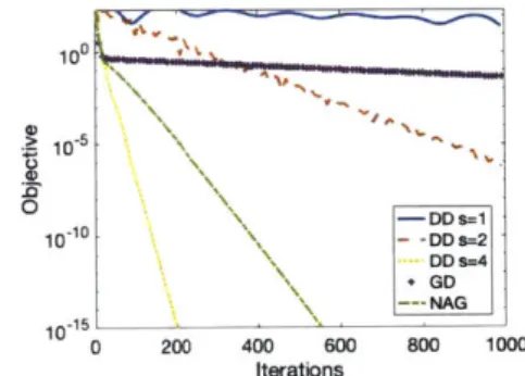
Convergence paths of GD, NAG, and the proposed direct discretization(DD) pro-cedure for minimizing the quadratic function f(x) = IIAx - bH1 2 are demonstrated in Figure 3-1(a). For the proposed method we consider integrators with different degrees, i.e., s E
{1,
2, 4}. Observe that GD eventually attains linear rate since the function is strongly convex around the optimal solution. NAG displays local acceleration close to the optimal point as mentioned in [Su et al., 2014, Attouch and Peypouquet, 2016]. For DD, if we simulate the ODE with an integrator of order s = 1, the algorithm is eventually unstable. This result is consistent with the claim in [Wibisono et al.,2016] and our theorem that requires the step size to scale with O(N-05.). Notice that
using a higher order integrator leads to a stable algorithm. Our theoretical results suggest that the convergence rate for s E
{1,
2, 4} should be worse than O(N--2) and one can approach such rate by making s sufficiently large. However, as shown in Fig-ure 3-1(a), in practice with an integrator of order s = 4, the DD algorithm achieves a convergence rate of O(N- 2). Hence, our theoretical convergence rate in Theorem 1 might be conservative.We also compare the performances of these algorithms when they are used to minimize
10 U 10-0 -GD -- NAG 20 DD s=1' 10- DD s=2 DD s=4 100 102 104 10 Iterations
(a) Quadratic objective
Figure 3-1: Convergence paths of GD, system with integrators of degree s Assumption 3.2.1 with p=2. a) 1 10 -GD -- NAG DD s=1 DD s=2 0-2 + DD s=2 DDs=4 100 102 104 106 Iterations (b) Objective as in (3.20)
NAG, and the proposed simulated dynamical
1, s = 2, and s = 4. The objectives satisfy
Matrix C and vector d are generated similarly as A and b. The result is shown in Figure 3-1(b). As expected, we note that GD no longer converges linearly, but the other methods converge at the same rate as in Figure 3-1(a).
Decoupling ODE coefficients with the objective
Throughout this paper, we assumed that the constant p in (3.11) is the same as the one in Assumption 3.2.1 to attain the best theoretical upper bounds. In this experiment, however, we empirically explore the convergence rate of discretizing the
ODE
2q + 1
+(t)
+ (t) + q2t 2Vf(x(t)) = 0,
when q
$
p. In particular, we use the same quadratic objective f(x) = flAx - b||2as in the previous section. This objective satisfies Assumption 3.2.1 with p = 2. We simulate the ODE with different values of q using the same numerical integrator with the same step size. Figure 3-2 summarizes the experimental results. We observe that when q > 2, the algorithm diverges. Even though the suboptimality along the continuous trajectory will converge at a rate of ((t-P) = ((t- 2), the discretized
10 0
0
10~10
10 0 102 106
Iterations
Figure 3-2: Minimizing quadratic objective by simulating different ODEs with the RK44 integrator (41h order). In the case when p = 2, the optimal choice for q is 2.
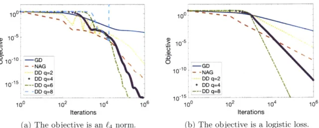
0 4) -0 10 --10-5 10-1 GD NAG DD q=21 + DD q=4 10- .---DD q=6 - -DDq=8 102 106 0 10-5 0-10 0 -GNAG DD q=2 *DD q=4 --- DD q=8\ 10 100 Iterations
(a) The objective is an f4 norm.
102 104
Iterations
(b) The objective is a logistic loss.
Figure 3-3: Experiment results for the cases that Assumption 3.2.1 holds for p > 2.
Beyond Nesterov's acceleration
In this section, we discretize ODEs with objective functions that satisfy Assumption
3.2.1 with p > 2. For all ODE discretization algorithms, we use an order-2 RK integrator that calls the gradient oracle twice per iteration. Then we run all algorithms for 106 iterations and show the results in Figure 3-3. As shown in Example 3.2.2, the objective
f(x) = JJAx - b (3.21)
satisfies Assumption 3.2.1 for p = 4. By Theorem 4.2.2 if we set q = 4, we can achieve a convergence rate close to the rate (N-4). We run the experiments with different
-DD q=2 - -DD q=3 - DD q=4 -DD q=5 100 106 10 4 1 10 4
values of q and summarize the results in Figure 3-3(a). Note that when q > 2, the convergence of direct discretization methods is faster than NAG. Interestingly, when
q = 6 > p = 4, the discretization is still stable with convergence rate roughly 09(N-5).
This suggests that our theorem may be conservative. We then simulate the ODE for the objective function
10
f
(x) = log(1 + e-'),i=1
for a dataset of linearly separable points. The data points are generated in the same way as in Section 3.2.4. As it satisfies Assumption 3.2.1 for arbitrary p > 0, in Figure
3-3(b), the objective decreases faster for larger q.
3.2.5
Technical lemmas of the proof
Proof of Proposition 3.2.1
According to the dynamical system in (3.12) we can write
= v, -= - I.V - p2tp-2Vf (x). (3.22)
t
Using these definitions we can show that
t2 2t t + . + t.\ =4p2(2v,i)+ 2(v,v)+2 x+-v-x,+x +-2p 2p 2p + pt- 1(f (x) - f(x*)) 2t2 K + 2p+ I 2t2 . 2p . t x t .2p+I . 4p2 t A p2 ( t +22p 2p t