Direct Tablet Formation by Electrospinning and
Compaction
by
Nicholas Matti Sondej
B.S. Mechanical Engineering, Georgia Institute of Technology (2012)
Submitted to the Department of Mechanical Engineering
in partial fulfillment of the requirements for the degree of
Master of Science in Mechanical Engineering
at the
MASSACHUSETTS INSTITUTE OF TECHNOLOGY
June 2014
@
Massachusetts Institute of Technology 2014. All rights reserved.
A
Author...
Certified by...
Signature redacted
I. ...
Department of Mechanical Engineering
May 9, 2014
Signature redacted
Alexander H. Slocum
Pappalardo Professor of Mechanical Engineering
Thesis Sypervisor
Signature redacted
A ccepted by ...
...
David E. Hardt
Ralph E. and Eloise F. Cross Professor of Mechanical Engineering
Chairman, Department Committee on Graduate Students
MASSACHUSETTS INSTmTUE OF TECHNOLOLGY
MAY 17 2015
LIBRARIES
Direct Tablet Formation by Electrospinning and Compaction
by
Nicholas Matti Sondej
Submitted to the Department of Mechanical Engineering on May 9, 2014, in partial fulfillment of the
requirements for the degree of
Master of Science in Mechanical Engineering
Abstract
A process and physical system were developed to manufacture pharmaceutical tablets through an electrospinning operation and subsequent compaction. Theoretical simu-lations of the electrospinning were run to predict physical system performance, and a proof-of-concept device was designed, produced and tested. The process was demon-strated to be theoretically scalable to levels of production suitable for industrial phar-maceutical manufacturing. The system demonstrated clear advantages over preexist-ing pharmaceutical manufacturpreexist-ing equipment, eliminatpreexist-ing airborne drug particulate matter, minimizing liquid drying time, and enabling a more agile, liquid-based con-tinuous manufacturing process to be utilized for pharmaceutical production. Future work was specified to refine and optimize the process, and improve process control and monitoring in order to meet the pharmaceutical industry's strict regulatory controls. Thesis Supervisor: Alexander H. Slocum
Acknowledgments
The sum total of my entire MIT experience would not have been possible without the crazy, inspiring, awesome and motivating personality that is of course, Profes-sor Alexander Slocum. I would like to thank Alex for pushing the entire Precision Engineering Research Group (PERG) to think differently and deterministically, to maintain a healthy balance of hard work, intense exercise and good company, and to give us a role model whom we worked hard for, not because we had to, but because he sets the highest bar for himself, and who are we not to attempt the same.
Thank you to Professor Bernhardt Trout for providing a most interesting, applied, industry research problem to work on for the past two years. It was the sort of work I had hoped to be able to do at MIT and your collaboration with Novartis made that possible.
I will always be in awe of the men and women of PERG, whose incredible successes and talents have inspired me to do more, to be more, and to learn more. If I pushed myself harder, it was always to try to catch up to each of you.
Special thanks goes to National Instruments, for their generous donation of NI data acquisition equipment towards the project, as well as to Professor David L. Trumper, of the MIT Precision Motion Control Laboratory, for facilitating commu-nication and the support from National Instruments.
I would especially like to thank Mark Belanger and the Edgerton Center Student Shop; Ken Stone, Hayami Arakawa and Brian Chan and the MIT Hobby Shop, and Pierce Hayward and the AMP Graduate Student Machine Shop for their continual technical support, use of machine shop facilities and endless patience throughout the process.
To my family - thank you for the support throughout this process. It took my attention away from you many times, yet you were always there throughout. Special thanks to Mom, for proof-reading one more paper, with the same mastery of eloquent, concise phrasing as ever.
making sure I always had enough baked goods, and sending me emails to ensure I didn't starve due to a lack of free food from around campus. It was a pleasure to drop by constantly and brighten your days, and have your never-ceasing support.
Finally, I owe my sanity, good health and energy to the men and women of the MIT Cycling and Triathlon Clubs who provided an outlet and release from the daily office grind with a more physically enjoyable form of delightful punishment.
Contents
1 Introduction
1.1 Objective . . . .
1.2 Batch vs. Continuous Manufacturing 1.3 Continuous Fiber Production . . . . 1.4 Single Needle Electrospinning . . . .
2 Theoretical Work
2.1 Background . . . . 2.2 Significant Parameters . . . .
2.3 Electric Field Approximations . . . .
2.4 2.5
2.6
2.3.1 Performance . . . . Electric Field Interference . . . . Electric Breakdown Voltage, Ventilation, and Safety . Manufacturing Considerations . . . .
3 Experimental Setup
3.1 Power and Pumping... 3.2 Spinneret . . . . 3.3 Collector Development... 3.4 Horizontal Collector Rod . . . . 3.5 Stripper Plate and Die Design 3.6 Collector Rod Rotation ... 3.7 Upper Punch and Compression
17 17 18 20 22 25 25 27 28 32 32 33 35 39 . . . . 4 0 . . . . 4 1 . . . . 4 2 . . . . 4 5 . . . . 4 7 . . . . 4 9 . . . . 5 0
3.8 D ie Plugs . . . . 50 3.9 Non-Conductive Stand . . . . 51 3.10 Material Selection . . . . 51 3.10.1 Delrin@ . . . . 51 3.10.2 Aluminum Alloy 6061-T6511 . . . . 52 3.10.3 316 Stainless Steel . . . . 53 3.10.4 01 Tool Steel . . . . 53 4 Experimental Methods 55 4.1 Solution Preparation . . . . 56
4.2 Critical Spinning Voltage Experiments . . . . 57
4.3 Horizontal Static Rod Characterization . . . . 58
4.4 Rotating Collector Rod Trials . . . . 59
4.5 Multiple Needle Rotating Collector Rod . . . . 59
4.6 Stripping Procedure . . . . 60
4.7 Tablet Compression . . . . 60
5 Results6 5.1 Critical Spinning Voltage . . . . 63
5.2 Horizontal Static Rod Experiments . . . . 65
5.3 HSR and Rotating Rod Comparison . . . . 65
5.4 Compression Results . . . . 67
6 Conclusion 69 7 Future Work 71 7.1 Continuous Process Monitoring by Machine Vision . . . . 71
7.2 Stripping Movements . . . . 72
7.3 Continuous Weight Monitoring . . . . 72
7.4 Solution Optimization for Improved Stripping Process . . . . 73
A Spinneret Design
A.1 Data Collection and System Monitoring and Control A.2 Spinneret Receiver v1.0 .
A.3 Integrated Spinneret Head A.4 Quick-Swap Head . . A.5 Integrated Spinneret Rece A.6 Quick-Swap Spinneret PIE A.7 Air Entanglement Vortex A.8 Ancillary Electrodes . . A.9 Die Floor Elevator . . . A.10 Die Punch and Post-Proc< A.11 Die Cavity and Ejector Pi A.12 Nozzle Geometry and Flo, A.13 Droplet Formation . . . A.14 Needle Arrays . . . . A.15 Contact Angles . . . . .
1.
and Head Unit
Compaction .
v2.0
B Electrostatic Field Modeling
B.1 Finite Element Solver Code . . . .
C Electrostatic Lensing
D Manufacturing Process Development Work
75 75 76 77 77 78 79 79 80 80 81 81 82 82 83 83 89 89 101 103 . . . .
. . .
List of Figures
1-1 High level view of research design space . . . . 18
1-2 Example batch production manufacturing process steps . . . . 19
1-3 Melt spinning production process detail, image courtesy of Textile Knowledge Innovation Platform . . . . 21
1-4 Generalized single needle electrospinning setup . . . . 23
1-5 Characteristic Taylor cone with labeled forces . . . . 24
2-1 'Lightning rod' style vertical rod collector . . . . 26
2-2 Applicable electrode-collector configurations for electric field approxi-m ations . . . . 29
2-3 Typical arrangement of interior node used in finite difference analysis 30 2-4 Comparison of theoretical field approximation (left) to simulation (right) 32 2-5 Isoperformal curve of production at specified 1 billion pill/year pro-duction rate . . . . 36
3-1 Overview of process components . . . . 39
3-2 Full experimental setup in experiment enclosure . . . . 40
3-3 Stainless steel dispensing needle used in final experiments . . . . 41
3-4 Spot size experiment, without ancillary electrodes, 180 mm diameter (left) and with best configuration, 30 mm diameter (right) . . . . 42
3-5 Direct-to-die electrospinning setup . . . . 43
3-6 Fiber deposition around die orifice at edge . . . . 43
3-7 Fiber deposition on elevated die floor . . . . 44
3-9 Cantilever beam with uniform load . . . . 46
3-10 Cut-away view of stripper plate and bearing surfaces . . . . 47
3-11 Minimum (left), and example negative die floor rake angle (right) 48 3-12 Normal force due to a positive (left) and negative rake angle (right) 48 3-13 Undesirable (left) and effective (right) stripper plate geometry . . . . 49
3-14 Delrin shaft connector detail . . . . 49
3-15 Sliding ground contact . . . . 50
3-16 Post-process compaction intermediate steps for a single pill compaction 50 3-17 Die plug detail . . . . 51
3-18 Non-conductive stand detail . . . . 52
4-1 Experimental procedure checklist . . . . 56
4-2 Horizontal static collector rod setup . . . . 59
4-3 Post-strip fiber 'tube' in die . . . . 61
4-4 Tableting press and die, die plug inserted . . . . 62
5-1 Critical spinning voltage versus spinneret collector distance . . . . 64
5-2 Critical spinning voltage versus solution flow rate . . . . 65
5-3 HSR electrospinning performance at various spinning parameters . . . 66
5-4 0.2 g spinning run by HSR (left) and rotating collector rod (right) 66 5-5 Example compression force versus punch distance profile . . . . 67
5-6 Variation in degree of compression across tablet surface, note frayed edge 68 5-7 Compressed tablets produced with varying spinning parameters . . . 68
A-1 Exploded views of the quick swap nozzle experimental setup . . . . . 75
A-2 Spinneret receiver detail . . . . 76
A-3 Integrated spinneret head detail . . . . 77
A-4 Quick-swap head detail . . . . 78
A-5 Integrated second generation spinneret receiver and head unit detail . 79 A-6 Quick-swap spinneret plates detail . . . . 79
A-8 Quick-swap head detail . . . . 84
A-9 Mechanism for retraction of die floor detail . . . . 85
A-10 Ancillary electrode and air entanglement vortex detail . . . . 86
A-11 Parameters of Bashforth-Adams equation on a cross-section of a sessile drop [1] . . . . 86
A-12 Example sessile drop picture taken with goniometer; 8 wt% 1.3MDa PVP and ethanol solution . . . . 87
C-1 Finite difference model of system with ancillary electrodes . . . . 101
C-2 Spinning results on ancillary electrodes . . . . 102
List of Tables
1.1 System functional requirements . . . . 18
4.1 Example solution recipe . . . . 57 4.2 Experiment run times by flow rate . . . . 59
Chapter 1
Introduction
In recent years, the pharmaceutical industry has begun to focus its research and development efforts on developing more efficient drug manufacturing processes. The impetus for this move is to accelerate the process of developing new drugs, as well as to enable pharmaceutical manufacturing facilities to respond faster to changes in market demand. Pharmaceutical manufacturing agility - the ability to produce pills in a large spectrum of different batch sizes and formulations - has become a significant functional requirement for next-generation processes. The industry seeks to both decrease the facility size and capital costs, and increase the flexibility of future manufacturing equipment. Current research has thus shifted away from the current batch manufacturing schema towards a completely different manufacturing paradigm
-continuous manufacturing -which has seen proven success in various other industries.
1.1
Objective
The goal of this research was to develop a continuous manufacturing process for producing pharmaceutical tablets. The design space for this research can be found in Figure 1-1. It required the system to accept, as an input, a viscous, drug-laden polymer solution from pre-existing upstream processes and produce discrete, solid tablets as output.
iden-r - - - m = I I I I I I I Project Design Space I I I I-... I I I
Figure 1-1: High level view of research design space
tified at an early stage in the design process. Table 1.1 displays these requirements, which were developed from analysis of the design space, as well as of the larger overall pharmaceutical manufacturing environment in which the system would perform.
Table 1.1: System functional requirements
1.2
Batch vs. Continuous Manufacturing
Batch production, as it is currently implemented in the pharmaceutical industry, in-volves numerous, discretized, serial processes, which are detailed by Figure 1-2. The label 'batch production' comes from the fact that individual pills are manufactured in a batch, which must pass entirely through a specific step in the overall process
Current powder-based systems produce ambient airborne API particulates which
Minimize airborne API produce a respiratory hazard to workers
particulates that the continuous system should reduce
Competitive production Novartis goal production rate is ability to
rate produce 1 billion pills per year
Upstream processes produce a liquid, polymeric solution from which the tableting system must produce solid, dry
Liquid-based tableting pills
System must be able to maintain 24/7 tableting operation with no downtime for
Continuous production duration of weeks at a time
before the next batch can be sent through. There are often bottlenecks in the batch production paradigm, as certain processes - often drying - take longer than others. This results in an inefficient manufacturing schema, as batches will either accumulate in inventory while waiting for a slower process, or faster processes must be run at re-duced rates, wasting manufacturing capability. However, this manufacturing schema has been ingrained in the pharmaceutical industry as the result of a combination of technological momentum and persistence, and a risk-averse regulatory environment which tends to discourage large technological changes.
ing- Granuation Drying Milling
Coating I -Compression Blending >
Figure 1-2: Example batch production manufacturing process steps
Batch production is a relatively inflexible manufacturing process, as it is currently implemented in the pharmaceutical industry. It is often used to produced powder-based pharmaceutical tablets - that is, tablets which are produced by filling a die cavity with a powder containing the drug products, and then compressing the powder into a hard, monolithic tablet. The capital equipment involved in such a manufac-turing paradigm is generally sized to the desired batch size, with different plants, or at least separate manufacturing lines, required to manufacture drugs of significantly different batch sizes. This is a problem, because a growing trend in the pharmaceuti-cal industry has been towards more user-specific, smaller batch treatments, which the current state of manufacturing technology is ill-equipped to produce cost-effectively. Continuous manufacturing is defined as a manufacturing process in which a con-stant supply of inputs to the process -generally raw materials or intermediate com-ponents - result in a proportionally constant supply of outputs in the form of finished products and any process waste. The economics of manufacturing theory categorize raw materials, intermediate components, and finished products that are in storage
as inventory, as financial liabilities, since they may depreciate in value over time and generate no income until they are either used in the production of finished goods, or sold. Continuous manufacturing reduces these inefficiencies, since intermediate com-ponents are inherently consumed by the manufacturing process at the same rate as they are created, and since there is a finer degree of control over production rate with a continuous system. Indeed, continuous manufacturing allows for much flexibility in adjusting production rate to market demand -any required changes in production rate can be implemented in the time it takes one pill to pass entirely through the manufacturing system. This offers a much faster response time than batch manufac-ture, where production rate changes can only be made after the entire current batch goes through the system. Additionally, since continuous manufacturing requires a constant flow of materials through the system, a liquid-based system becomes more appropriate as compared to current powder-based technology.
1.3
Continuous Fiber Production
A significant proportion of both current and future pharmaceutical manufacturing time is dedicated to drying liquid solutions into solid products. In batch production, the entire pharmaceutical batch is dried at once and subsequent processes simply wait on the drying step to complete. Drying time becomes a much more important variable in continuous production, because the entire manufacturing process occurs simulta-neously in serial and can only run as quickly as drying can be accomplished. Thus, a process to rapidly dry a continuous solid product from a viscous liquid precursor is desired. Inspiration was drawn from various spinning processes in the synthetic fiber industry, with electrospinnning chosen as the best suited process for the pharmaceu-tical industry.
Continuous production of polymer products has already been achieved in the synthetic fiber industry through a variety of processes, including melt spinning, wet spinning, and electrospinning. Melt spinning is widely used to produce artificial fibers for use in nylon and other synthetic fabrics. The process, which is illustrated in
Figure 1-3, involves heating a thermoplastic polymer beyond its melting point, then extruding the liquid melt through a plate with numerous orifices to form a shower of small diameter liquid streams.
To VfiMer
Figure 1-3: Melt spinning production process detail, image courtesy of Textile
Knowl-edge Innovation Platform
The self-weight of the streams causes a stretching that elongates the fibers in the axial direction and reduces their diameter. As the streams are passed through a chamber of cooling gas, the increased surface area to volume ratio as well as decreased mass per unit length of stream allows the stream to quickly cool and form a thin fiber. The melt spinning process is extremely efficient and can be used for high-throughput fiber production, but the temperature increase necessary for the process can dam-age certain heat-sensitive active pharmaceutical ingredients (API). Additionally the equipment needed for melt spinning can span several stories of a building, in order
to provide sufficient height to fully cool and solidify the resultant fibers.
A more compact process with similar physical characteristics and results, but without the API-damaging heating of melt spinning, is electrospinning. The electro-spinning process involves the controlled
jetting
of one or many dry micro- or nano-scale fibers from an electrically charged, liquid solution of dissolved material and itssolvent, under the influence of a high-voltage electric field. Electrospinning is attrac-tive as a continuous manufacturing process to the pharmaceutical industry due to several key characteristics of the process that fulfill several currently unmet needs in the industry. The solvent used to liquefy the fiber material can be fully evaporated in a distance on the order of 300 mm, instead of a few stories, shrinking the manufac-turing equipment size. The electrostatic attraction of the charged API and polymer solution to a grounded collector ensures a near-complete delivery of drug product from spinneret to end destination. This allows both precise delivery of API-laden fibers to a desired spatial location, as well as minimizing the amount of airborne pharmaceu-tical particulate matter present in the manufacturing environment. Environmental pharmaceutical dust is a health hazard for workers in pharmaceutical manufacturing plants, and new manufacturing processes are sought which reduce worker exposure to airborne particulates containing APIs.
1.4
Single Needle Electrospinning
Single needle electrospinning is one of the simplest electrospinning processes. In a single needle setup, spinning solution is pumped through a single conductive needle charged to a high voltage at a measured flowrate. The process is illustrated in Figure
1-4.
The needle is fixtured at a specified distance from a grounded metal collector. As pressure is applied to a fluid reservoir coupled to the needle, a droplet forms on the tip of the needle. The droplet is subject to opposing forces including surface tension, which adheres the droplet to the tip of the needle, and electrostatic force and gravity, in the case of a vertically-oriented system, which pull the droplet downwards towards the collector. If the electrode voltage were to be increased gradually from zero, the droplet can be observed to deform into a characteristic Taylor cone, after Geoffrey Taylor. A Taylor cone, with labeled forces, can be found in Figure 1-5.
At a critical electrode voltage, surface tension forces are overcome by electrostatic forces and a liquid jet will emit from the droplet formed at the tip of the needle. This
Needle Tip
Grounded
Collector
+ kV Plate
Figure 1-4: Generalized single needle electrospinning setup
jet carries the liquid solution away from the needle tip at a flow rate governed by the process parameters, which will be discussed in more detail later on.
There are three operating modes in which the electrospinning process can proceed. If the flow rate pumped through the needle is equal to the flow rate of solution carried away through the jetting process, electrospinning is carried out at steady state. This equal flow rate situation is considered the optimum operating regime for continuous manufacturing, because it ensures production of consistent fibers, a critical functional requirement of any pharmaceutical manufacturing process. At an operating voltage greater than the critical voltage, if the flow rate of solution supplied is less than the flow rate of solution jetted, the droplet will decrease in size. The Taylor cone from which jetting occurs may actually ascend into the barrel of the needle in this operating regime. This operating regime is considered marginally acceptable, since it will result in the production of fibers, but it is sub-optimal because of the lower production rate and the potential inability to visually monitor the Taylor cone. Machine vision is a proposed mechanism for efficient process monitoring, but it cannot be used in this operating regime. The third operating mode results from a pumped flow rate higher than that of the jetting capacity of a particular equipment setup and results in an oscillation between brief moments of spinning combined with frequent dripping of
Needle Barrel
Fs.,rface Tension FsurfaceTension
-Taylor Cone
FElectrostatic
Figure 1-5: Characteristic Taylor cone with labeled forces
Chapter 2
Theoretical Work
2.1
Background
The goal of analysis work on this research was to validate assumptions about the nature of the electrospinning phenomena that the system was based on, in addition to developing virtual prototyping and forecasting tools to quickly iterate through po-tential designs. The models were used to ensure that physical experiment failures and successes could be used to make informed conclusions. Additionally, process calcula-tions allowed the prototype system to be sized correctly and inferences to be drawn concerning the future scalability of the process to full-scale industrial manufacturing. Initial work focused on spinneret designs, and the accompanying modeling work focused on fundamental physics at the nozzle tip. Characterization research on nozzle design, multi-needle arraying, and the physics of droplet formation on surfaces was performed, all of which can be found in Appendix A. It was discovered that spinneret optimization had an insignificant effect on fiber spinning performance, but the tools developed for this first phase, such as the electrostatic field finite difference solver described later in this chapter were flexible enough to be adapted for use in later phases.
The next logical research focus was designing a collector which would encourage preferential fiber deposition inside a pill die cavity. While there was some demonstra-ble success at focusing the electrospun fibers, efforts to deposit the fibers precisely
Figure 2-1: 'Lightning rod' style vertical rod collector
into the die cavity failed. The significant obstacle in this phase was producing elec-tric fields which could force the electrospun fibers to concentrate in tight formation along a central axis in order to enter a small orifice. The electric field modeling tools developed previously were used to size the diameter, location and applied voltage of additional field-shaping electrodes designed to focus spun fibers towards the die orifice. A vertical rod collector sticking out of the die, detailed in Figure 2-1, had the most promising performance, but still fell short of the functionality desired.
The results of the 'lightning rod' style collector did build a foundation for the design of the final system configuration, as it was the first example of a collector that could translate through the pill die and provide enough clearance between the walls of the die and the collector for deposited fiber material trapped by the rod. Additionally, this collector design demonstrated that conducting surface areas were gradually insulated by the deposition of spun fibers, since the ability of the collector to entrap fiber material became worse as more fiber was deposited.
2.2
Significant Parameters
The electrospinning process was discovered over 100 years ago, and in more contem-porary times has been studied extensively since Taylor published his initial models of electrically-driven jets in 1969 [9]. Subsequent research [3], [7], [8] has identified the following parameters which have varying demonstrable effects on the electrospinning process, in no order of significance:
" Applied electrode voltage
" Spinneret to collector (SC) gap distance " Solution volumetric flow rate
" Solution dielectric constant " Solution viscosity
" Ambient temperature " Ambient relative humidity " Collector geometry
Solution and environment parameters were controlled by utilizing a constant so-lution formulation, and by running blocks of experiments on the same day. This was done because environmental parameters were not found to significantly affect exper-imental results on an experiment to experiment basis, and literature [2] had shown that electrospinning of a large variety of solutions was possible. Controlling for the above variables resulted in a set of four process parameters from which to design experiments:
" Applied electrode voltage
" Spinneret to collector spacing distance " Solution volumetric flow rate
2.3
Electric Field Approximations
The thin jets of spinning solution emitting from the spinneret head are electrically charged, and as such, electrostatic fields significantly influence their trajectories. Elec-trostatic fields which guide spun fibers towards the collector are thus preferential. A finite difference (FD) solver was written in MATLAB to aid design visualization of the electrostatic fields generated by the experimental setups. The code can be found in Appendix B. The solver allows rapid virtual prototyping of different collector and electrode designs and quickly displays the electrostatic fields which will be generated by the modeled configuration.
Electrostatic theory offers four basic field approximations applicable to potential embodiments of this electrospinning system with which to validate the FD solver, as
shown in Figures 2-2(a), 2-2(b), 2-2(c) and 2-2(d).
Initial work to characterize the performance of different spinneret designs used a large 300 mm x 300 mm aluminum plate as a collector, a length scale which was significantly larger than the spinneret, which had a characteristic length on the order of 25 mm or less. With such a small characteristic length, especially in comparison to the spinneret-collector (SC) distance ranges of similar published research [3], [5], [10] of 150-400mm, these setups could be approximated by a point-plate configuration, as seen in Figure 2-2(b).
The final, horizontal rod design is a hybrid of two of these approximations. Viewed down the axial direction of the collector rod, the field lines are approximated by a point-point configuration as seen in Figure 2-2(d). If the final system is viewed from a transverse direction, with the full length of the collector rod in view, the electrostatic fields appear as in Figure 2-2(b).
The actual FD solver builds an array of equations, defined by the matrix:
A<D = b (2.1)
where A is a (Z -R) x (Z -R) coefficients matrix, where Z is the number of nodes in the z-direction and R is the number of nodes in the r-direction, D is a column vector
(a) Plate-Plate (b) Point-Plate
(c) Plate-Point (d) Point-Point
Figure 2-2: Applicable electrode-collector configurations for electric field approxima-tions
of the unknown electrostatic potentials at each node and b is a column vector of constants, which is equal to specific voltages at the boundary nodes of known voltage, and zero everywhere else. The solver first fills the coefficients matrix and constants column vector and then solves for the potentials in <b using matrix manipulation in
MATLAB.
Populating the matrices for subsequent calculation involved creating a mesh of nodes at different spatial points in a virtual representation of the experiment geometry and treating them as surrounded by differential elements. A typical interior node, that is, a node which did not lay on the control volume boundary, can be seen in
Figure 2.3.
As can be seen in Figure 2.3, as the finite difference analysis is in progress, a control volume was defined around the current node, Nz,r, which is the central node
(Z -1 ,A) .(Z, R-1) . (Z, R) . (Z, R +1) I I I I I I I I I (Z+1, R)
Figure 2-3: Typical arrangement of interior node used in finite difference analysis
in the figure. The voltage at this, and each node was calculated using Gauss' Law
(2.2):
V-E= p (2.2)
60
where E is the electric field vector, p is the total charge density inside the control volume in question and co is the permittivity of free space, or electric constant of the material contained in the control volume, in this case, air. Since all charge in the system, which includes by definition both the charge on the electrified spinneret head, and the lack of charge on the grounded collector, lies on the boundary of the
control volume, p = 0 and thus (2.2) reduces to the Laplace equation (2.3):
V - E = 0 (2.3)
In the case of the rectangular mesh in the FD solver, this equation signifies that the sum of the derivative of the electric field with respect to both the radial and axial directions is zero. Thus, no electric field can be 'stored' in the control volume and all electric fields generated by voltage differences between the current node and its neighbors must sum to zero:
Ez-i,r + Ez,r+i + Ez+i,r + Ezr1 = 0
In short, (2.4) states that all fields that enter the differential element must also leave it. The electric field created between two different electrostatic potentials is:
E =-V 4-
=-(-+
&D)
(2.5)az
Or
where <D is the electrostatic potential, which is a scalar field defined at each node point. Equation (2.5) enables the calculation of all four of the electric fields created by the voltage differences between the current node, and its neighbors. The FD solver approximates the partial derivatives found in (2.5) by using the definition of the derivative:
- IZ+AZ -
(2.6)
az
Az(26Substituting (2.6) and (2.5) into (2.4) yields the governing FD equation for an interior node:
z-1,r - (Dz,r
+
'z,r+1 - z,r+
z+1,r
- + C,r-l --z,r z,r 0 (2.7)Az + A '- A zr+ Ar = 27
Equation (2.7) simplifies into:
Ar<Dz_1,r + Az4z,r+i + ArI~z+i,r + AZ(Iz,r-i
+
(z,r(-2Az - 2Ar) = 0 (2.8)which allows the A and b matrices of (2.1) to be populated in the FD code.
Boundary Conditions
In the analysis, the boundary conditions for the spinneret and the collector were known, while those at the edges of the control volume were chosen to strike a balance between accuracy and rapid calculation, since the electrostatic effects near the edge (2.4)
of the control volume were not important to the performance of the system. The boundary nodes which fell on either the spinneret head or the collector were specified with either the experiment voltage or ground respectively, while the field was assumed to be constant, V1b = 0 at the other boundaries.
2.3.1
Performance
The first simulations replicated the theoretical field line configurations of Figure 2.3 in order to validate the code's functionality. The results from these initial simulations
were satisfactory, as an example point-plate simulation in Figure 2-4.
0.02
-0.06 -0.04 402 S 0.02 0.04 0.06
Figure 2-4: Comparison of theoretical field approximation (left) to simulation (right)
Once developed and validated, the FD code was then used to simulate the variation of different experimental parameters, such as the spinneret-collector gap distance, applied spinneret voltage, collector rod diameter, and the effects of additional ring electrodes to test their potential influence on the generated electric fields.
2.4
Electric Field Interference
The system developed in this research is meant to be implemented as a single cell in an array of parallel modules in a manufacturing setup. As the electrospinning setup is static, there is no risk of mechanical interference between each module in a parallel manufacturing scheme. Electrostatic interference is a potential issue when running multiple cells together, if the modules are spaced too closely. This can result in adverse effects in all modules, or inconsistent spinning in the modules at either end
of a linear array of modules, due to edge effects. As was mentioned previously, the spinneret needles can be modeled as point charges, the electric field between which is described by Coulomb's Law as:
Q
()
(2.9)
-47reo Ir2
Where k is the vector field of electric field strength,
Q
is the charge on the point charge, co is the electric permittivity of free space, ? is the unit vector from the charge in the direction of the point at which the field strength is being measured, and Irlis the magnitude of the distance from the charge to the point in space where the electric field strength is being measured. Most importantly, it can be observed from Equation 2.9 that electric field strength decays as a function of 1/Ir 12 from the charge which is generating the field. With this in mind, at a distance of 300 mm horizontally from the spinneret, which is the typical SC distance, the electric field is 1/9000 of that at the spinneret, so a design which spaces modules at roughly the same length scale as the SC distance should produce minimal electrical interference. This assumption is later tested when performing electrospinning runs with two spinnerets in the final horizontal collector rod design.
2.5
Electric Breakdown Voltage, Ventilation, and
Safety
There are significant safety concerns that accompany the generation of a high voltage electrode in an enclosure filled with evaporated volatile organic compounds. The electric breakdown voltage - the voltage at which electrical arcing will occur, and ignition is possible - in ambient air was first calculated to ensure that experiments never positioned the spinneret closer to the collector than a distance equal to three times the electric breakdown distance of air at 50 kV, the maximum voltage that the experimental power supply could provide. The calculation starts with an assumption of a uniform field, such as that between two parallel plates. While this is not an
accurate physical representation of a system with a needle spinneret and a collector, any electrical arcing will occur along the centerline of the setup, where the electrode and collector are closest. Along this centerline, the fields are equivalent for a parallel plate setup and a point and plate setup, so the assumption is valid. The uniform electric field between two parallel plates is represented by Equation 2.10:
E V - (2.10)
d
Where E is the electric field strength, V is the applied voltage and d is the distance between the spinneret and collector (SC distance). The critical electric field at which point breakdown will occur in air, Ec, is roughly 3 kV/mm [4]. The minimum safe SC distance is desired so Equation 2.10 is first solved for the distance between the two, at the maximum voltage which the power supply can provide:
dmin = Vmax (2.11)
Ec
Where dmin is the minimum safe SC distance and Vmax is the maximum possible applied voltage. Substituting the known values leaves:
50 kV
dmin = = 16.7mm (2.12)
3 ky/mm
Since this calculation was based upon an assumed model with a safety factor of one, and the breakdown distance can be affected by humidity and other factors, a safety factor of three was chosen. Thus a SC distance of greater than 51 mm will prevent electrical breakdown. Since the typical SC distance was 300 mm, this was well within a safe region.
Proper ventilation of the experiment enclosure was also important. The enclosure was a 0.6m x 0.6 m x 0.9 m (2 ft x 2 ft x 3 ft nominal) box made from cast acrylic sheets, for a total volume of 0.324 m3 (12 ft3 nominal). The box was attached to building ventilation which removed 1.13 m3/min (40 cfm nominal) of atmosphere from the enclosure. Thus the air handling system was replacing the air in the enclosure over three times per minute, while an amount of ethanol solvent several orders of
magnitude smaller than the volume of the enclosure was added to the enclosure per minute.
2.6
Manufacturing Considerations
The ultimate goal of this electrospinning research is to produce a new system and manufacturing process for use in pharmaceutical production. Although the primary aim of this work was to produce a single functional cell, specifications were also developed for the full system in which it would be a component. Novartis specified that a proof-of-concept system must be scalable to a production rate of 1 billion pills per year. A series of spreadsheets was developed to produce these process calculations and the MATLAB code used to generate some of the following graphs can be found in Appendix D. The first milestone in this process was to identify the high level parameters which would result in the system meeting this functional production goal. The overall production rate of the electrospinning process, and subsequent design of individual cells, is governed by two variables: the mass flow rate of solution through each module, and the number of modules spinning in parallel, and is given as
mapi,total = Nmodules rnapi,module (2.13)
Where Nmodules is the number of modules in parallel, r api,total is the overall active pharmaceutical ingredient (API) production rate in [g/hr] and rhapi,module is the API mass flow rate per module.
At a prescribed total API production rate, Equation 2.13 produces a manufactur-ing isoperformal curve at the given rate. This curve describes all pairs of parameters which will result in the system meeting the specific target production rate. This isoperformal curve is displayed in Figure 2-5. It allows the number of modules in parallel, or the flow rate per module to be chosen, with the isoperformal curve then specifying the value of the other variable in order to exactly hit the production rate goal. Since the module flow rate will be a parameter in experimental testing, and will be more adjustable than the number of modules in the final system, it will be
considered the independent variable when deriving the equation for this curve. 2 X0 1.8 1.6 1.4 1.2 --' 0.8 . z 0.6 0.4 0.2 Vs 5 2 2.'S 3 A 4' 45 R owat e[mglmin]
Figure 2-5: Isoperformal curve of production at specified 1 billion pill/year production rate
Starting with the characteristic system equation, Equation 2.13 can be rearranged to solve for the number of modules required:
Nmodues = rnapi,total
mapi,module
The total specified API flow rate, rhapi,total is known, but the API mass flow rate
per module must be solved for. Fortunately this can be determined from the total volumetric liquid flow rate per module, which is also known. The API mass flow rate is
mapi,module mhmodule * Wapi
(2.15)
Where T
module is the total mass flow rate of liquid emanating from each module
and Wapi is the weight percent of API in the solution being spun. The total module mass flow rate can be determined from the total module volumetric flow rate
rnmodule = Qmodule -Psolution (2.16) Where Qmodule is the volumetric flow rate of the entire module, a specified param-eter, and psolution is the density of the entire solution before solvent evaporation. The density of polymer solutions may depend on the enthalpy of mixing of the solution constituents. However, as a simple approximation, a simpler method will be used to approximate the solution density by weighting the individual densities of the solution constituents by their weight percent as follows
mconstituent
- Mconstituent (2.17)
wsolution
mconstituent Vconstituent
Wconstituent -Pconstituent -Pconstituent - (2.18)
Msolution Msolution
Vapi Vpoiymner Vsoivent __ 1Vsiio
+ + - - (Vai + Volymer + Vsoivent) Vsoluton
Msolution Msolution Msolution Msolution Msolution
(2.19)
Psolution - Mouin(2.20)
Vsolution (Wapi -Papi + Wpolymer -Ppolymer + Wsolvent Psoivent)
Substituting Equations 2.15, 2.16, and 2.17 into the rearranged characteristic system equation, Equation 2.14 yields the governing equation for the isoperformal curve:
Nmodules = napi ,totai .(napi -Papi + Wpolymer -Ppolymer + Wsolvent -Psoivent) (2.21) Qapi -Wapi
Chapter 3
Experimental Setup
The experimental setup was designed to be a prototype of a single pharmaceutical pill manufacturing cell. The setup was designed with scalability in mind, allowing many cells to be run in parallel to meet production goals. The system performs three separate functions. It electrospins polymeric fiber laden with an active pharmaceutical ingredient (API) from an electrically charged spinneret to a grounded collector rod. Upon the completion of the spinning process, the rod is withdrawn into a pill die, where a stripper plate at the bottom of the die strips the pharmaceutical material from the rod. Finally, an upper punch descends into the die and the material is compressed into a final tablet geometry. Fig. 3-1 provides a an overview diagram detailing the steps in this process which will be explained in further detail in following sections.
Spin Strip Compress Eject
The full experimental setup with final, rotating, horizontal collector rod configu-ration is displayed in Figure 3-2.
Figure 3-2: Full experimental setup in experiment enclosure
3.1
Power and Pumping
Electrospinning requires both a high voltage power supply and a source of pumping head. Electric potential was supplied by a 50 kV, 20 W benchtop power supply
(Gamma High Voltage Research ES50P-20W/DDRM/PRG). The polymer solution
was pumped via a syringe pump (Harvard Apparatus PHD2000 Infusion), through a length of tubing and finally through the system spinneret.
3.2
Spinneret
The spinneret in an electrospinning setup is an electrically conductive part that is charged to the applied spinning voltage, and from which the spinning solution forms jets. Initial research focused on new spinneret head designs as the primary driver of electrospinning process performance, and a series of increasingly detailed spinneret heads with various spinning nozzle geometries were designed, produced and tested. The design process, iterations and test results from these experiments can be found in Appendix A. However, the test results from these experiment trials found that these spinneret designs had little influence on fiber drying and collection, which was instead driven mainly by collector geometry. This seemed to result from the fact that the nozzle designs only affected the geometry and number of the fluid jets at their origin, while the electric fields generated by the collector geometry affected the fiber during its entire trajectory. All subsequent research focused on optimizing the embodiment of the collector, as it was found that collector design could enable a much higher degree of control over fiber deposition. Once the design focus shifted to the collector and die, electrospinning experiments were carried out with stainless steel blunt-end needles, with all final trials carried out specifically with 25 gauge needles, Figure 3-3, in order to constrain differences in electrospinning performance to changes in the collector design.
3.3
Collector Development
The design of the collector underwent a series of iterations, beginning as an aluminum plate, continuing as an aluminum plug inside a pill die, to its final embodiment as a horizontal rod, described in Section 3.4. The successes and failures of each iteration drove the design of the next collector.
The first collector plate design was a 300 mm x 300 mm square aluminum plate. Experiments with the plate collector characterized the 'spot size' of the needle spin-nerets, as detailed in Figure 3-4. The spot size is the maximum dimension of the circular distribution of fiber material desposited on the collector. Baseline spot size measurements were taken from simple electrospinning setups with a needle and the plate collector. Additional ancillary ring electrodes were added in later experiments on electrostatic lensing, in order to focus the applied electric fields and shrink the spot size. Efforts to shrink the spot size did reduce the characteristic diameter of the spot from around 180 mm to 30 mm, but a plate collector was not found to produce fiber deposition which could easily be transformed into common tablet geometries.
U
Figure 3-4: Spot size experiment, without ancillary electrodes, 180 mm diameter (left) and with best configuration, 30 mm diameter (right)
The goal of the second design was a collector that would promote easy tablet formation, and which utilized the electrostatic focusing electrodes from the collector plate setup. This iteration attempted to deposit the spun fibers directly into a pill die orifice, a setup which can be found in Figure 3-5.
The goal of this design was to produce electric fields which concentrated the fibers along the central axis of the setup by the time the fibers arrived at the die mouth,
Figure 3-5: Direct-to-die electrospinning setup
and collect on an aluminum plug at the bottom of the die that formed the die floor. Experimental results demonstrated only a partial success at the stated goals of this collector design. While fibers were concentrated at the die orifice, they had a tendency to collect on the edge of the orifice, as seen in Figure 3-6, where there was a sharp edge and thus a slight electric field concentration. Fiber deposition inside the die itself was minimal.
Figure 3-6: Fiber deposition around die orifice at edge
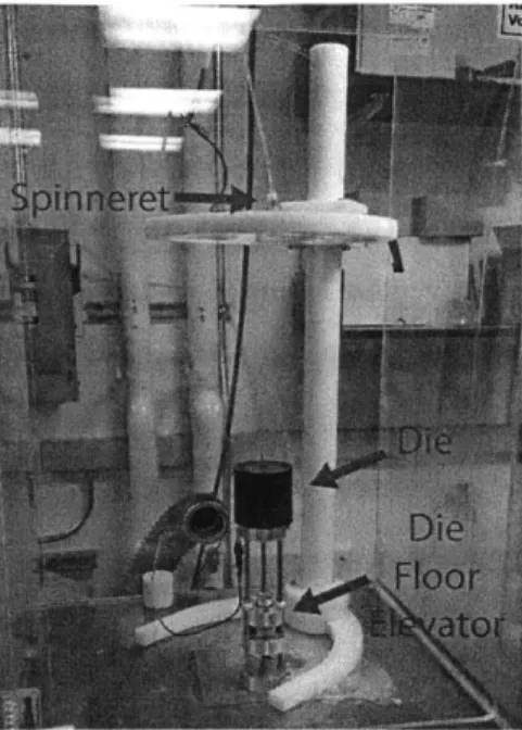
collector was an issue in the direct-to-die system, so a die floor elevator was developed that could re-position the aluminum plug in the die cavity. This enabled the die floor to translate up and down with respect to the die. Experiments were run with the die floor located at the upper surface of the die cavity, as well as with the plug slowly descending into the die. This succeeded in producing a much tighter fiber deposition pattern on the aluminum plug, but both experiment runs resulted in laying down too much fiber outside of the collector plug, as displayed in Figure 3-7 to be successfully implemented as a commercial process.
Figure 3-7: Fiber deposition on elevated die floor
At this point, inspiration was drawn from lightning rods, whose purpose is to provide the path of least electrical resistance in a volume of space. While the exper-iments in this research avoid the electrical breakdown and arcing found in lightning strikes, a similar collector design which provides a focal point for an electrostatically-driven process is desired. Thus a collector was developed in which a 50 mm long thin rod, smaller than the diameter of the 12 mm tableting die, projected out from the tableting die, with the ability to withdraw into the die during or after the spinning process. The rod was aligned axially with the electrospinning needle, and experimen-tal trials found it lacked the ability to effectively collect electrospun fibers in a useful
manner. However, it was proposed to rotate this collector 900, which resulted in the final horizontal rod collector design.
3.4
Horizontal Collector Rod
The collector used in the final setup, Figure 3-8, is a 3.76 mm (0.148 in. nominal) diameter rod, 600 mm long, which is mounted horizontally, perpendicular to the axial direction of the electrospinning needle.
Figure 3-8: Horizontal collector rod
The rod is composed of a hard (Rockwell B89, see material properties section) multipurpose 01 tool steel, a design decision made to ensure that the stripping action of the rod passing through the stripper plate, described below, does not mar the surface of the collector and cause a reduced capability to strip. The most significant feature of the collector rod is its orientation perpendicular in relation to the spinneret. This configuration presents a 600 mm long surface on which to deposit fibers.
This collector configuration is cantilevered from the tableting die, and will suffer from some deflection due to self-weight. The loading situation can be accurately modeled as a cantilever beam with a uniformly-distributed load, as seen in Figure 3-9.
Theory from structural mechanics, Equation 3.1, describes the maximum tip de-flection of the beam in this configuration:
Amax = 1 (3.1)
/---
Al
,Imax
R
Figure 3-9: Cantilever beam with uniform load
Where Am, is the maximum deflection of the beam, w is the beam weight per unit length, 1 is the beam length, E is the modulus of elasticity and I is the cross-sectional moment of inertia. Equation 3.2 is the moment of inertia, I for a beam of circular cross section:
I = rd4 (3.2)
64
Where d is the rod diameter. At a rod diameter of 3.76 mm and length of 600 mm, the max deflection at the tip of an 01 tool steel collector rod is 0.75 mm, less than 0.25% of the distance between the spinneret and collector. This ensures that any deflection of the unsupported side of the collector rod is unlikely to cause any fiber distribution issues, since it results in a minuscule difference in spinneret-collector distance.
This collector embodiment has several advantages over current collector designs, such as conductive belts or flat metal plates, because it encourages fiber collection in a geometry that is well suited for simple and rapid post-spin transfer to a pill die. In comparison, the process of transferring a sheet of electrospun mat material collected
on a planar surface to a cylindrical die cavity is non-trivial and may require many intermediate folding steps.
3.5
Stripper Plate and Die Design
The tableting die component of this system contains features designed to smoothly strip fiber material from the collector rod and then compress it into the final pill geometry. The die used in final experimental trials had an inner cavity diameter of 12 mm. The floor of the die consists of a metal plate with a hole in the center, whose diameter creates a precision slip fit with the collector rod. The shape of this plate forms a negative of the desired geometry of the bottom half of the final tablet. A cut-away cross section of an example die, detailing the stripper plate feature and bearing surfaces can be seen in Figure 3-10.
Adapter Plug Stripper Plate
Collector Rod
Relief Gap
Journal Bearing
Figure 3-10: Cut-away view of stripper plate and bearing surfaces
The design of the bearing surfaces seen in Figure 3-10 is notable because of the spacing between the stripper plate and journal bearing. The two bearing surfaces are designed according to Saint-Venant's Principle, which suggests a ratio of 1.6:1 or greater for the spacing of linear bearings to the diameter of the shaft, to
mini-mize bearing lock-up and premature failure due to offset loading. In the final design presented here, the minimum spacing between the two bearing surfaces is 9.65 mm,
compared with a collector rod diameter of 3.76 mm, for a ratio of 2.5:1, well above the 1.6:1 minimum acceptable ratio suggested by Saint-Venant.
The rim of the central hole in the stripper plate is ground to a sharp edge in order to effectively strip the fiber from the collector rod. Due to the desired domed or cylindrical pill geometries produced via this system, the stripper edge will always form a rake angle of < 00 with the collector rod, as seen in Fig. 3-11.
,p nFi er S Depun Fibe
Figure 3-11: Minimum (left), and example negative die floor rake angle (right)
A negative rake angle is less ideal than a positive rake angle in this scenario, since the force produced normal to the cutting surface tends to compress the fiber material against the collector rod, rather than lifting it off of the rod as in the case of a positive rake angle, see Figure 3-12.
Figure 3-12: Normal force due to a positive (left) and negative rake angle (right)
Since the geometries of standard tablet shapes require the cutting edge to form a non-ideal neutral or negative rake angle, a sharp edge is important to ensure that the stripper plate overcomes the adhesive force attaching the fibers to the rod, rather than shearing the fibers themselves and allowing a skin of fibers to pass beneath the floor of the die. Fig. 3-13 demonstrates an example of acceptable sharp edge and an example of unacceptable worn edge geometry.
A 316 stainless steel washer served as the stripper plate for prototyping purposes, in order to quickly replace defective or failed plates, but stripper plate was designed to be made from a case-hardened stainless steel in production models for increased
Figure 3-13: Undesirable (left) and effective (right) stripper plate geometry wear resistance.
3.6
Collector Rod Rotation
Electrospinning process tests with a static, horizontal collector rod demonstrated that while the the horizontal rod entraps nearly all fibers spun during the process, it does so with unequal distribution about the circumference of the rod. This in turn had a tendency to produce inhomogeneous pills with uneven mechanical properties across the width of the pill, since the fiber material was unevenly distributed in the die after the stripping process. To solve this problem, a DC motor was attached to the collector rod via an insulating Delrin shaft connector, as seen in Figure 3-14.
Figure 3-14: Delrin shaft connector detail
The collector rod could no longer be grounded by an alligator clip since it was rotating, so a conductive sliding contact was attached to the end of the collector rod, as seen in Figure 3-15. This allowed the collector to main electrical contact with ground while rotating.
Figure 3-15: Sliding ground contact
3.7
Upper Punch and Compression
A tableting press (Gamlen Tableting GPT1) was adapted to provide the compression force for the prototype system. Pill dies were designed to interface with the press and a 12 mm diameter die was built to perform with a corresponding punch. The tableting press provided a simple measurement of compaction force as a function of position of the punch. The punch compressed the fiber material until the onboard load cell detected that the desired load limit had been achieved. The compaction process is detailed in Figure 3-16.
Figure 3-16: Post-process compaction intermediate steps for a single pill compaction
3.8
Die Plugs
Since the collector rod could not fit in the tableting press used in the compression experiments, a small plug was created to form the die floor for the tableting dies during compression. The plug replaced the functionality of a withdrawn collector rod that would be present in a scaled-up version of the setup. The die plug can be seen in Figure 3-17.
Figure 3-17: Die plug detail
3.9
Non-Conductive Stand
The experimental setup is designed such that the electric fields that drive the elec-trospinning process are as close to axisymmetric around the spinning needle as can be reasonably achieved. As such, the stand used to suspend the needle must be non-conductive to avoid creating a secondary induced electrostatic field. The stand design is detailed in Figure 3-18. The stand includes a vertical scale to determine the spinneret to collector (SC) distance as well an adjustable clamp to vary the SC parameter. A cantilevered arm design was used to hold the spinneret receiver to facilitate frequent SC adjustment via the single compression clamp. A gantry-style design was first considered but was rejected in favor of the cantilever design due to the decreased adjustment time and effort required to change the SC distance with the cantilever-style stand.
3.10
Material Selection
3.10.1
Delrin@
Delrin@has excellent electrically insulating properties and is both highly machinable and structurally rigid. It was an attractive material choice for the experimental stand, as it minimized distortion of the electric fields generated in experiments.
Figure 3-18: Non-conductive stand detail
3.10.2
Aluminum Alloy 6061-T6511
Aluminum 6061-T6511 was chosen as the metal for prototype development for its mechanical properties. Aluminum alloy 6061 exhibits excellent machinability. The T6511 temper includes a solution heat treatment, artificial aging, and internal stress-relief treatment performed by stretching [6]. This temper ensures that the alloy will undergo minimal physical change due to internal forces and reactions of surface chemistry post-machining, producing parts that meet the design tolerances. Alu-minum 6061-T6511's properties are:
" Hardness: Rockwell B60
" Yield Strength: 276 MPa