Linear inverse problems with various noise models and mixed regularizations

HAL Id: hal-01080093

https://hal.archives-ouvertes.fr/hal-01080093

Submitted on 4 Nov 2014

HAL is a multi-disciplinary open access

archive for the deposit and dissemination of

sci-entific research documents, whether they are

pub-lished or not. The documents may come from

teaching and research institutions in France or

abroad, or from public or private research centers.

L’archive ouverte pluridisciplinaire HAL, est

destinée au dépôt et à la diffusion de documents

scientifiques de niveau recherche, publiés ou non,

émanant des établissements d’enseignement et de

recherche français ou étrangers, des laboratoires

publics ou privés.

Linear inverse problems with various noise models and

mixed regularizations

François-Xavier Dupé, Jalal M. Fadili, Jean-Luc Starck

To cite this version:

François-Xavier Dupé, Jalal M. Fadili, Jean-Luc Starck. Linear inverse problems with various noise

models and mixed regularizations. 1st InternationalWorkshop on New Computational Methods for

Inverse Problems, May 2011, Cachan, France. �10.4108/icst.valuetools.2011.246491�. �hal-01080093�

Linear inverse problems with various noise models and

mixed regularizations

François-Xavier Dupé

francois-xavier.dupe@cea.fr

Jalal M. Fadili

Jalal.Fadili@greyc.ensicaen.fr

Jean-Luc Starck

jean-luc.starck@cea.fr

ABSTRACT

In this paper, we propose two algorithms to solve a large class of linear inverse problems when the observations are corrupted by various types of noises. A proper data fidelity term (log-likelihood) is introduced to reflect the statistics of the noise (e.g. Gaussian, Poisson, multiplicative, etc.) inde-pendently of the degradation operator. On the other hand, the regularization is constructed through different terms re-flecting a priori knowledge on the images. Piecing together the data fidelity and the prior terms, the solution to the inverse problem is cast as the minimization of a composite non-smooth convex objective functional. We establish the well-posedness of the optimization problem, characterize the corresponding minimizers for different kind of noises. Then we solve it by means of primal and primal-dual proximal splitting algorithms originating from the field of non-smooth convex optimization theory. Experimental results on decon-volution, inpainting and denoising with some comparison to prior methods are also reported.

Keywords

Inverse Problems, Poisson noise, Gaussian noise, Multiplica-tive noise, Duality, Proximity operator, Sparsity.

1.

INTRODUCTION

Previous work A lot of works have already been dedicated to linear inverse problems with Gaussian noise (see [16] for a comprehensive review), while linear inverse problems in presence of other kind of noise such as Poisson noise have attracted less interest, presumably because noises properties are more complicated to handle. Such inverse problems have however important applications in imaging such as restora-tion (e.g. deconvolurestora-tion in medical and astronomical imag-ing), or reconstruction (e.g. computerized tomography). Since the work for Gaussian noise by [9], many other meth-ods have appeared for managing linear inverse problem with sparsity regularization. But they limited to the Gaussian

case. In the context of Poisson linear inverse problems using sparsity-promoting regularization, a few recent algorithms have been proposed. For example, [11] stabilize the noise and proposed a family of nested schemes relying upon prox-imal splitting algorithms (Forward-Backward and Douglas-Rachford) to solve the corresponding optimization problem. The work of [4] is in the same vein. These methods may be extended to other kind of noise. However, nested algorithms are time-consuming since they necessitate to sub-iterate. Using the augmented Lagrangian method with the alter-nating method of multipliers algorithm (ADMM), which is nothing but the Douglas-Rachford splitting applied to the Fenchel-Rockafellar dual problem, [13] presented a deconvo-lution algorithm with TV and sparsity regularization, and [1] a denoising algorithm for multiplicative noise. This scheme however necessitates to solve a least-square problem which can be done explicitly only in some cases.

Contributions In this paper, we propose a framework for solving linear inverse problems when the observations are corrupted by various types of noise. In order to form the data fidelity term, we take the exact likelihood associated to the noise model. As a prior, the images are assumed to comply with several regularity properties or/and con-straints reflecting knowledge about the original image. The solution to the inverse problem is cast as the minimization of a composite non-smooth convex functional, for which we prove well-posedness of the optimization problem, character-ize the corresponding minimcharacter-izers, and solve them by means of primal and primal-dual proximal splitting algorithms orig-inating from the realm of non-smooth convex optimization theory. Convergence of the algorithms is also shown. Ex-perimental results and comparison to other algorithms on deconvolution are finally conducted.

Notation and terminology Let H a real Hilbert space, here a finite dimensional vector subspace of Rn_{. We denote}

by k.k the norm associated with the inner product in H, and I is the identity operator on H. k.k_p, p ≥ 1 is the ℓp

norm. x and α are respectively reordered vectors of image samples and transform coefficients. We denote by ri C the relative interior of a convex set C. A real-valued function f is coercive, if limkxk→+∞f (x) = +∞, and is proper if its

domain is non-empty dom f = {x ∈ H | f (x) < +∞} 6= ∅. Γ0(H) is the class of all proper lower semicontinuous

(lsc) convex functions from H to (−∞, +∞]. We denote by |||M||| = maxx6=0kMxk_kxk the spectral norm of the linear

kernel.

Let x ∈ H be a n-pixels image. x can be written as the superposition of elementary atoms ϕγparameterized by γ ∈

I such that x =P_γ∈Iαγϕγ = Φα, |I| = L, L > n. We

denote by Φ : H′ _{→ H the dictionary (typically a frame of}

H), whose columns are the atoms all normalized to a unit ℓ2-norm

2.

PROBLEM STATEMENT

Consider the image formation model where an input image of n pixels x is indirectly observed through the action of a bounded linear operator H : H → K, with K a real Hilbert space (usually a subspace of Rm_{, m > 0), and contaminated}

by a noise ε through a composition operator ⊙ (e.g. addi-tion),

y ∼ Hx ⊙ ε . (1) The linear inverse problem at hand is to reconstruct x from the observed image y.

A natural way to attack this problem would be to adopt a maximum a posteriori (MAP) bayesian framework with an appropriate likelihood function — the distribution of the ob-served data y given an original x — reflecting the statistics of the noise. As a prior, the image is supposed to be eco-nomically (sparsely) represented in a pre-chosen dictionary Φ as measured by a sparsity-promoting penalty Ψ supposed throughout to be convex but non-smooth, e.g. the ℓ1 norm.

2.1

Gaussian noise case

For Gaussian noise, we consider the following formation model, y = Hx + ε , (2) where ε ∼ N (0, σ2_).

>From the probability density function, the negative log-likelihood writes:

fGaussian : η ∈ H 7→ kη − yk22/(2σ

2_{) . (3)}

>From this function, we can directly derive the following result,

Proposition 1. fGaussianis a proper, strictly convex and

lsc function.

2.2

Poisson noise case

The observed image is then a discrete collection of counts y = (y[i])16i6n which are bounded, i.e. y ∈ ℓ∞. Each

count y[i] is a realization of an independent Poisson random variable with a mean (Hx)i. Formally, this writes in a vector

form as

y ∼ P(Hx) . (4)

>From the probability density function of a Poisson random variable, the likelihood writes:

p(y|x) =Y

i

((Hx)[i])y[i]_{exp (−(Hx)[i])}

y[i]! . (5)

Taking the negative log-likelihood, we arrive at the following data fidelity term:

fPoisson : η ∈ H 7→

n

X

i=1

fp(η[i]), (6)

if y[i] > 0, fp(η[i]) =−y[i] log(η[i]) + η[i] if η[i] > 0,_{+∞ otherwise,}

if y[i] = 0, fp(η[i]) =



η[i] if η[i] ∈ [0, +∞), +∞ otherwise.

Using classical results from convex theory, we can show that,

Proposition 2. fPoissonis a proper, convex and lsc

func-tion. fPoissonis strictly convex if and only if∀i ∈ {1, . . . , n},

y[i] 6= 0.

2.3

Multiplicative noise

We consider here the same context of multiplicative as in [1]. With multiplicative noise, a usual approach to improve the signal to noise ratio consists in averaging independent obser-vation of the same resolution. When considering SAR/SAS system, this method is called multilook, i.e. M -look in the case of the averaging of M images. For fully developed speckle, the averaged images are Gamma distributed,

y = xε, ε ∼ Γ(M, 1/M ) . (7)

In order to simplify the problem, the logarithm of the ob-servation is considered,

log(y) = log(x) + log(ε) = z + ω . (8) And in [1], the authors proof that the anti log-likelihood yields,

fMulti : η ∈ H 7→ M

n

X

i=1

(z[i] + exp(log(y[i]) − z[i]) . (9)

Using classical results from convex theory, we can directly derive,

Proposition 3. fMulti is a proper, strictly convex and lsc

function.

2.4

Optimization problem

Our aim is then to solve the following optimization prob-lems, under a synthesis-type sparsity prior1_{where H}′_{is the}

Hilbert space defined by the dictionary, argmin α∈H′ J(α), J : α 7→ f1◦ H ◦ Φ(α) + K X i=1 Ri(α) . (Pf1,γ,ψ)

The data fidelity term f1 reflect the noise statistics and the

Ri, 1 6 i 6 K the K prior terms. In this paper, we restrict

to the case K = 2, with K1 = Ψ, the penalty function Ψ :

α 7→ PL_i=0ψi(α[i]) which is positive, additive, and chosen 1_{Our framework and algorithms extend to an analysis-type}

to enforce sparsity, γ > 0 is a regularization parameter and K2= ıC◦ Φ the indicator function of the convex set C (e.g.

the positive orthant for Poissonian data).

For the rest of the paper, we assume that f1is a proper,

con-vex and lsc function, i.e. f1∈ Γ0(H). This is true for many

kind of noises including Poisson, Gaussian, Laplacian. . . (see [3] for others examples).

>From the objective in (Pf1,γ,ψ), we get the following,

Proposition 4.

(i) f1is a convex functions and so are f1◦H and f1◦H◦Φ.

(ii) Suppose that f1 is strictly convex, then f1◦ H ◦ Φ

re-mains strictly convex if Φ is an orthobasis and ker(H) = ∅.

(iii) Suppose that (0, +∞) ∩ H ([0, +∞)) 6= ∅. Then J ∈ Γ0(H).

2.5

Well-posedness of

Let M be the set of minimizers of problem (Pf1,γ,ψ).

Sup-pose that Ψ is coercive. Thus J is coercive. Therefore, the following holds:

Proposition 5.

(i) Existence: (Pf1,γ,ψ) has at least one solution, i.e. M 6=

∅.

(ii) Uniqueness: (Pf1,γ,ψ) has a unique solution if Ψ is

strictly convex, or under (ii) of Proposition 4.

3.

ITERATIVE MINIMIZATION

ALGORITHMS

3.1

Proximal calculus

We are now ready to describe the proximal splitting algo-rithms to solve (Pf1,γ,ψ). At the heart of the splitting

frame-work is the notion of proximity operator.

Definition 6 ([14]). Let F ∈ Γ0(H). Then, for every

x ∈ H, the function y 7→ F (y) + kx − yk2₂/2 achieves its infimum at a unique point denoted by prox_Fx. The operator prox_F : H → H thus defined is the proximity operator of F . Then, the proximity operator of the indicator function of a convex set is merely its orthogonal projector. One important property of this operator is the separability property:

Lemma 7 ([7]).

Let Fk∈ Γ0(H), k ∈ {1, · · · , K} and let G : (xk)16k6K 7→

P

kFk(xk). Then proxG= (proxFk)16k6K.

For Gaussian noise, we can easily prove that with f1 as

de-fined in (3),

Lemma 8. Let y be the observation, the proximity op-erator associated to fGaussian (i.e. the Gaussian anti

log-likelihood) is,

prox_βfGaussianx = βy + σ

2_x

β + σ2 . (10)

The following result can be proved easily by solving the prox-imal optimization problem in Definition 6 with f1as defined

in (6), see also [5].

Lemma 9. Let y be the count map (i.e. the observa-tions), the proximity operator associated to fPoisson(i.e. the

Poisson anti log-likelihood) is,

prox_βfPoissonx = x[i] − β + p (x[i] − β)2_{+ 4βy[i]} 2 ! 16i6n . (11)

As with multiplicative noise fMulti involves the exponential,

we need the W-Lambert function [8] in order to derive a closed form of the proximity operator,

Lemma 10. Let y be the observations, the proximity op-erator associated to fMulti is,

prox_βfMultix =`x[i] − βM −

W (−βM exp(x[i] − log(y[i]) − βM ))´_16i6n, (12) where W is the W-Lambert function, i.e. the function such that W(a) exp(W(a)) = a, a ∈ R.

We now turn to prox_γΨwhich is given by Lemma 7 and the following result:

Theorem 11 ([12]). Suppose that ∀ i: (i) ψiis convex

even-symmetric, non-negative and non-decreasing on R+_,

and ψi(0) = 0; (ii) ψi is twice differentiable on R \ {0}; (iii)

ψiis continuous on R, and admits a positive right derivative

at zero ψ′_{i +}(0) = lim_h→0+ψi_h(h) > 0. Then, the proximity

operator prox_δψi(β) = ˆα(β) has exactly one continuous

so-lution decoupled in each coordinate β[i] :

ˆ α[i] = ( 0 if |β[i]| 6 δψi +′ (0) βi− δψ ′ i( ˆα[i]) if |β[i]| > δψ ′ i +(0) (13)

Among the most popular penalty functions ψisatisfying the

above requirements, we have ψi(α[i]) = |α[i]| , ∀ i, in which

case the associated proximity operator is soft-thresholding, denoted ST in the sequel.

3.2

Splitting on the primal problem

3.2.1

Splitting for sums of convex functions

Suppose that the objective to be minimized can be expressed as the sum of K functions in Γ0(H), verifying domain

qual-ification conditions: argmin x∈H F (x) = K X k=1 Fk(x) ! . (14)

Proximal splitting methods for solving (14) are iterative al-gorithms which may evaluate the individual proximity oper-ators prox_Fk, supposed to have an explicit convenient struc-ture, but never proximity operators of sums of the Fk.

Splitting algorithms have an extensive literature since the 1970’s, where the case K = 2 predominates. Usually, split-ting algorithms handling K > 2 have either explicitly or implicitly relied on reduction of (18) to the case K = 2 in the product space HK_{. For instance, applying the}

Douglas-Rachford splitting to the reduced form produces Spingarn’s method, which performs independent proximal steps on each Fk, and then computes the next iterate by essentially

aver-aging the individual proximity operators. The scheme de-scribed in [6] is very similar in spirit to Spingarn’s method, with some refinements.

3.2.2

Application to noisy inverse problems

Problem (Pf1,γ,ψ) is amenable to the form (14), by wisely

introducing auxiliary variables. As (Pf1,γ,ψ) involves two

linear operators (Φ and H), we need two of them, that we define as x1 = Φα and x2 = Hx1. The idea is to get rid

of the composition of Φ and H. Let the two linear opera-tors L1 = [I 0 − Φ] and L2 = [−H I 0]. Then, the

optimization problem (Pf1,γ,ψ) can be equivalently written:

argmin (x1,x2,α)∈H×K×H′ f1(x2) + ıC(x1) + γΨ(α) | {z } G(x1,x2,α) + (15) ıker L1(x1, x2, α) + ıker L2(x1, x2, α) , (16)

where ıker Li are the indicatrice function of the kernel space

of the operator Li, in others words these two indicatrice

functions will enforce the equality constraints x1= Φα and

x2 = Hx1. Notice that in our case K = 3 by virtue of

separability of the proximity operator of G in x1, x2 and α;

see Lemma 7.

Algorithm 1: Primal scheme for solving (Pf1,γ,ψ).

Parameters: The observed image y, the dictionary Φ, number of iterations Niter, µ > 0 and regularization

parameter γ > 0. Initialization:

∀i ∈ {1, 2, 3}, p(0,i)= (0, 0, 0)T. z0= (0, 0, 0)T.

Main iteration: For t = 0 to Niter− 1,

• Data fidelity (Lemmas 8, 9 and 10):

ξ(t,1)[1] = proxµf1/3(p(t,1)[1]).

• Sparsity-penalty (Lemma 11):

ξ(t,1)[2] = proxµγΨ/3(p(t,1)[2]).

• Positivity constraint: ξ(t,1)[3] = PC(p(t,1)[3]).

• Auxiliary constraints with L1 and L2: (Lemma 12):

ξ(t,2)= Pker L1(p(t,2)), ξ(t,3)= Pker L2(p(t,3)).

• Average the proximity operators:

ξt= (ξ(t,1)+ ξ(t,2)+ ξ(t,3))/3.

• Choose θt∈]0, 2[.

• Update the components:

∀i ∈ {1, 2, 3}, p(t+1,i)= p(t,i)+ θt(2ξt− zt− ξ(t,i)).

• Update the coefficients estimate: zt+1= zt+ θt(ξt− zt).

End main iteration

Output: Reconstructed image x⋆= zNiter[0].

The proximity operators of f1 and Ψ are easily accessible

through Lemmas 8, 9, 10 and 11. The projector onto C is trivial for most of the case (e.g. positive orthant, closed

interval). It remains now to compute the projector on ker Li,

i = 1, 2, which by well-known linear algebra arguments, is obtained from the projector onto the image of L∗

i.

Lemma 12. The proximity operator associated to ıker Li

is

Pker Li= I − L

∗

i(Li◦ L∗i)−1Li . (17)

The inverse in the expression of Pker L1is (I+Φ◦Φ

T₎−1_can

be computed efficiently when Φ is a tight frame. Similarly, for L2, the inverse writes (I+H◦H∗)−1, and its computation

can be done in the domain where H is diagonal; e.g. Fourier for convolution or pixel domain for mask.

Finally, the main steps of our primal scheme are summarized in Algorithm 1. Its convergence is a corollary of [6][Theo-rem 3.4].

Proposition 13. Let (zt)t∈N be a sequence generated by

Algorithm 1. Suppose that Proposition 4-(iii) is verified, and P

t∈Nθt(2 − θt) = +∞. Then (zt)t∈N converges to a

(non-strict) global minimizer of (Pf1,γ,ψ).

3.2.3

Splitting on the dual: Primal-dual algorithm

Our problem (Pf1,γ,ψ) can also be rewritten in the form,

argmin α∈H′ F ◦ K(α) + γΨ(α) (18) where now K = „ H ◦ Φ Φ « and F : (x1, x2) 7→ f1(x1) +

ıC(x2). Again, one may notice that the proximity operator

of F can be directly computed using the separability in x1

and x2.

Recently, a primal-dual scheme, which turns to be a pre-conditioned version of ADMM, to minimize objectives of the form (18) was proposed in [2]. Transposed to our setting, this scheme gives the steps summarized in Algorithm 2. Adapting the arguments of [2], convergence of the sequence (αt)t∈Ngenerated by Algorithm 2 is ensured.

Proposition 14. Suppose that Proposition 4-(iii) holds. Let ζ = |||Φ|||2(1 + |||H|||2), choose τ > 0 and σ such that στ ζ < 1, and let (αt)t∈R as defined by Algorithm 2. Then,

(α)t∈Nconverges to a (non-strict) global minimizer (Pf1,γ,ψ)

at the rate O(1/t) on the restricted duality gap.

3.3

Discussion

Algorithm 1 and 2 share some similarities, but exhibit also important differences. For instance, the primal-dual algo-rithm enjoys a convergence rate that is not known for the primal algorithm. Furthermore, the latter necessitates two operator inversions that can only be done efficiently for some Φ and H, while the former involves only application of these linear operators and their adjoints. Consequently, Algo-rithm 2 can virtually handle any inverse problem with a bounded linear H. In case where the inverses can be done efficiently, e.g. deconvolution with a tight frame, both algo-rithms have comparable computational burden. In general,

if other regularizations/constraints are imposed on the solu-tion, in the form of additional proper lsc convex terms that would appear in (Pf1,γ,ψ), both algorithms still apply by

introducing wisely chosen auxiliary variables.

Algorithm 2: Primal-dual scheme for solving (Pf1,γ,ψ).

Parameters: The observed image y, the dictionary Φ, number of iterations Niter, proximal steps σ > 0 and τ > 0,

and regularization parameter γ > 0. Initialization:

α0= ¯α0= 0 ξ0= η0= 0.

Main iteration: For t = 0 to Niter− 1,

• Data fidelity (Lemmas 8, 9 and 10): ξt+1= (I − σ proxf1/σ)(ξt/σ + H ◦ Φ ¯αt). • Positivity constraint: ηt+1= (I − σPC)(ηt/σ + Φ ¯αt). • Sparsity-penalty (Lemma 11): αt+1= proxτ γΨ ` αt− τ ΦT(H∗ξt+1+ ηt+1)´.

• Update the coefficients estimate: ¯αt+1= 2αt+1− αt

End main iteration

Output: Reconstructed image x⋆_{= Φα} Niter.

4.

EXPERIMENTAL RESULTS

4.1

Deconvolution under Poisson noise

Our algorithms were applied to deconvolution. In all ex-periments, Ψ was the ℓ1-norm. Table 1 summarizes the

mean absolute error (MAE) and the execution times for an astronomical image, where the dictionary consisted of the wavelet transform (here the translation-invariant discret wavelet transform which form a tight frame and so is a re-dundant transform) and the PSF was that of the Hubble telescope. Our algorithms were compared to state-of-the-art alternatives in the literature. In summary, flexibility of our framework and the fact that Poisson noise was handled properly, demonstrate the capabilities of our approach, and allow our algorithms to compare very favorably with other competitors. The computational burden of our approaches is also among the lowest, typically faster than the PIDAL algorithm [13]. Fig. 1 displays the objective as a function of the iteration number and times (in s). We can clearly see that Algorithm 2 converges faster than Algorithm 1.

RL-MRS [15] RL-TV [10] StabG [11] PIDAL-FS [13] MAE 63.5 52.8 43 43.6 Times 230s 4.3s 311s 342s Alg. 1 Alg. 2 MAE 46 43.6 Times 183s 154s

Table 1: MAE and execution times for the deconvo-lution of the sky image.

4.2

Inpainting with Gaussian noise

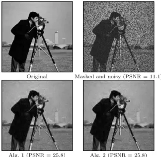
We also applied our algorithms to inpainting with Gaussian noise. In all experiments, Ψ was the ℓ1-norm. Fig 2

sum-marizes the results with the PSNR and the execution times for the Cameraman, where the dictionary consisted of the same wavelet transform as used for deconvolution and the mask was create from a random process (here with about 34% of missing pixels). Notice that both algorithms leads to the same solution which gives a good reconstruction of

100 101 102 103 ï6 ï5 ï4 ï3 ï2 ï1 0x 10 8 Iterations ALG1 ALG2 10ï4 10ï2 100 102 104 ï6 ï5 ï4 ï3 ï2 ï1 0x 10 8 Seconds

Figure 1: Objective function for deconvolution un-der Poisson noise in function of iterations (left) and times (right).

the image. Fig. 3 displays the objective as a function of the iteration number and times (in s). Again, we can clearly see that Algorithm 2 converges faster than Algorithm 1.

Original Masked and noisy (PSNR = 11.1)

Alg. 1 (PSNR = 25.8) Alg. 2 (PSNR = 25.8)

Figure 2: Inpainting results for the Cameraman us-ing our two algorithms.

4.3

Denoising with Multiplicative noise

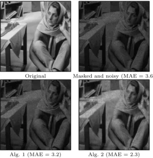
As imply by (8), the final estimate for each algorithm is given by taking the exponential of the result. In all exper-iments, Ψ was the ℓ1-norm. The Barbara image was set to

a maximal intensity of 30 and the minimal to a non-zero value in order to avoid issues with the logarithm. The noise was added using M = 10 which leads to a medium level of noise. Fig 4 summarizes the results with the MAE and the execution times for Barbara, where the dictionary consisted of the curvelets transform. The difference between the vi-sual results of the two algorithms can be explain be the fact we did not stop at the convergence, but instead stop after one thousand iterations. Our methods give correct recon-struction of the image. Fig. 5 displays the objective as a function of the iteration number and times (in s). Again, we can clearly see that Algorithm 2 converges faster than Algorithm 1.

0 200 400 600 800 1000 1200 0 2 4 6 8 10 12 14x 10 5 Iterations ALG1 ALG2 0 50 100 150 200 250 0 2 4 6 8 10 12 14x 10 5 Seconds

Figure 3: Objective function for inpainting with Gaussian noise in function of iterations (left) and times (right).

Original Masked and noisy (MAE = 3.6)

Alg. 1 (MAE = 3.2) Alg. 2 (MAE = 2.3)

Figure 4: Denoising results for Barbara using our two algorithms.

In this paper, we proposed two provably convergent algo-rithms for solving the linear inverse problems with a sparsity prior. The primal-dual proximal splitting algorithm seems to perform better in terms of convergence speed than the pri-mal one. Moreover, its computational burden is lower than most comparable of state-of-art methods. Inverse problems with multiplicative noise does not enter currently in this framework, we will consider its adaptation to such problems in future work.

6.

REFERENCES

[1] J. Bioucas-Dias and M. Figueiredo. Multiplicative noise removal using variable splitting and constrained optimization. IEEE Transactions on Image

Processing, 19(7):1720–1730, 2010.

[2] A. Chambolle and T. Pock. A first-order primal-dual algorithm for convex problems with applications to imaging. Technical report, CMAP, Ecole

Polytechnique, 2010.

[3] C. Chaux, P. L. Combettes, J.-C. Pesquet, and V. R. Wajs. A variational formulation for frame-based inverse problems. Inv. Prob., 23:1495–1518, 2007. [4] C. Chaux, J.-C. Pesquet, and N. Pustelnik. Nested

100 101 102 103 0.5 1 1.5 2 2.5 3 3.5 4x 10 7 Iterations ALG1 ALG2 100 101 102 103 104 0.5 1 1.5 2 2.5 3 3.5 4x 10 7 Seconds

Figure 5: Objective function for denoising with mul-tiplicative noise in function of iterations (left) and times (right).

iterative algorithms for convex constrained image recovery problems. SIAM Journal on Imaging Sciences, 2(2):730–762, 2009.

[5] P. L. Combettes and J.-. Pesquet. A Douglas-Rachford splittting approach to nonsmooth convex variational signal recovery. IEEE Journal of Selected Topics in Signal Processing, 1(4):564–574, 2007.

[6] P. L. Combettes and J.-C. Pesquet. A proximal decomposition method for solving convex variational inverse problems. Inverse Problems, 24(6), 2008. [7] P. L. Combettes and V. R. Wajs. Signal recovery by

proximal forward-backward splitting. SIAM Multiscale Model. Simul., 4(4):1168–1200, 2005.

[8] R. Corless, G. Gonnet, D. Hare, D. Jeffrey, and D. Knuth. On the Lambert W function. Advances in Computational Mathematics, 5:329–359, 1996. 10.1007/BF02124750.

[9] I. Daubechies, M. Defrise, and C. D. Mol. An iterative thresholding algorithm for linear inverse problems with a sparsity constraints. Comm. Pure Appl. Math., 112:1413–1541, 2004.

[10] N. Dey, L. Blanc-F´eraud, J. Zerubia, C. Zimmer, J.-C. Olivo-Marin, and Z. Kam. A deconvolution method for confocal microscopy with total variation regularization. In IEEE ISBI, pages 1223–1226, Arlington, USA, 15-18 April 2004.

[11] F.-X. Dup´e, M.-J. Fadili, and J.-L. Starck. A proximal iteration for deconvolving poisson noisy images using sparse representations. IEEE Transactions on Image Processing, 18(2):310–321, 2009.

[12] M. Fadili, J.-L. Starck, and F. Murtagh. Inpainting and zooming using sparse representations. The Computer Journal, 52(1):64–79, 2007.

[13] M. Figueiredo and J. Bioucas-Dias. Restoration of poissonian images using alternating direction optimization. IEEE Transactions on Image Processing, 19(12), 2010.

[14] J.-J. Moreau. Fonctions convexes duales et points proximaux dans un espace hilbertien. CRAS S´er. A Math., 255:2897–2899, 1962.

[15] J.-L. Starck and F. Murtagh. Astronomical Image and Data Analysis. Springer, 2006.

[16] J.-L. Starck, F. Murtagh, and M. Fadili. Sparse Signal and Image Processing: Wavelets, Curvelets and Morphological Diversity. Cambridge University Press, Cambridge, UK, 2010. in press.