Numerical and the MU radar estimations of gravity wave enhancement and turbulent ozone fluxes near the tropopause

HAL Id: hal-00317735

https://hal.archives-ouvertes.fr/hal-00317735

Submitted on 29 Nov 2004

HAL is a multi-disciplinary open access

archive for the deposit and dissemination of

sci-entific research documents, whether they are

pub-lished or not. The documents may come from

teaching and research institutions in France or

abroad, or from public or private research centers.

L’archive ouverte pluridisciplinaire HAL, est

destinée au dépôt et à la diffusion de documents

scientifiques de niveau recherche, publiés ou non,

émanant des établissements d’enseignement et de

recherche français ou étrangers, des laboratoires

publics ou privés.

wave enhancement and turbulent ozone fluxes near the

tropopause

Nikolai M. Gavrilov, S. Fukao

To cite this version:

Nikolai M. Gavrilov, S. Fukao. Numerical and the MU radar estimations of gravity wave enhancement

and turbulent ozone fluxes near the tropopause. Annales Geophysicae, European Geosciences Union,

2004, 22 (11), pp.3889-3898. �hal-00317735�

Annales Geophysicae (2004) 22: 3889–3898 SRef-ID: 1432-0576/ag/2004-22-3889 © European Geosciences Union 2004

Annales

Geophysicae

Numerical and the MU radar estimations of gravity wave

enhancement and turbulent ozone fluxes near the tropopause

1_{Saint-Petersburg State University, Atmospheric Physics Department, Petrodvorets, 198 504, St. Petersburg, Russia} 2_{Kyoto University, Center for Atmospheric and Space Research, Uji, Kyoto 611, Japan}

Received: 2 December 2003 – Revised: 18 June 2004 – Accepted: 24 June 2004 – Published: 29 November 2004 Part of Special Issue “10th International Workshop on Technical and Scientific Aspects of MST Radar (MST10)”

Abstract. It is shown with a numerical simulation that a

sharp increase in the vertical temperature gradient and Brunt-V¨ais¨al¨a frequency near the tropopause may produce an in-crease in the amplitudes of internal gravity waves (IGWs) propagating upward from the troposphere, wave breaking and generation of stronger turbulence. This may enhance the transport of admixtures between the troposphere and strato-sphere in the middle latitudes. Turbulent diffusion coefficient calculated numerically and measured with the MU radar are of 1–10 m2/s in different seasons in Shigaraki, Japan (35◦N, 136◦E). These values lead to the estimation of vertical ozone flux from the stratosphere to the troposphere of (1–10)×1014, which may substantially add to the usually supposed ozone downward transport with the general atmospheric circula-tion. Therefore, local enhancements of IGW intensity and turbulence at tropospheric altitudes over mountains due to their orographic excitation and due to other wave sources may lead to the changes in tropospheric and total ozone over different regions.

Key words. Meteorology and atmospheric dynamics

(Tur-bulence; Waves and tides) – Atmospheric composition and structure (Middle atmosphere composition and chemistry)

1 Introduction

One of the important problems is the role of gravity waves and turbulence in diffusion of ozone and gas species in the tropo-stratosphere. It is supposed recently that the main mechanism of the transport of admixtures influencing the ozone layer between the troposphere and the stratosphere is the general circulation of the atmosphere, creating up-ward motions near the equator and downup-ward motions at the middle and high latitudes (Holton, 1990). Additional ozone transport from the stratosphere to the troposphere could be produced by mesoscale and small-scale processes (Lamarque Correspondence to: N. M. Gavrilov

(gavrilov@pobox.spbu.ru)

and Hess, 2003). Mesometeorological processes may pro-duce intrusions of stratospheric ozone into the troposphere, which are frequently observed (Lamarque and Hess, 2003). Small-scale turbulence provides mixing of atmospheric gases and may produce turbulent ozone fluxes due to vertical gra-dients of the ozone mixing ratio (Pavelin et al., 2002; White-way et al., 2003). But despite intensive research during the last years, there are still many uncertainties and unknowns about the role which mesoscale and small-scale processes may play in the stratospheric-tropospheric exchange.

A boundary between the troposphere and the stratosphere is denoted as the tropopause. Usually it is located not far from the temperature minimum. There are several defini-tions of the tropopause based on temperature structure and dynamical features of the atmosphere (Dameris, 2003). The heights obtained with different tropopause definitions may be approximately equal (Birner et al., 2002), or sometimes they may differ up to several kilometers. Therefore, in gen-eral, we should say about a quite thick. One of the impor-tant features is a sharp increase in potential temperature and its vertical gradient in the tropopause region (Birner et al., 2002). This makes the mean temperature profile above the tropopause much more stable than below, which commonly assumes turbulence suppression above the tropopause.

On the other hand, experiments with radars, balloons and aircrafts (Pavelin et al., 2001; Pavelin and Whiteway, 2002; Luce et al., 2002) show strong internal gravity waves (IGWs) and unstable turbulized layers near and above the tropopause. Maxima of IGW activity and turbulent diffusivity near the tropopause were systematically observed during multiyear observations with Japanese Middle and Upper (MU) Atmo-sphere radar in Shigaraki (Fukao et al., 1994; Murayama et al., 1994; Kurosaki et al., 1996).

In this paper we analyze IGW theory to show that the sharp change in the vertical temperature gradient near the tropopause temperature minimum can make a sharp increase in the amplitudes of IGWs propagating upwards from the tro-posphere. This can lead to IGW breaking and to generation of stronger turbulence, which may make the tropopause more

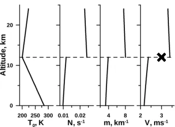
200 250 300 T0, K 0 10 20 A lti tu d e , k m 0.01 0.02 N, s-1 2 3 V, ms-1 4 8 m, km-1

Fig. 1. Simple model of temperature profile, Brunt-V¨ais¨al¨a

fre-quency, IGWs vertical wavenumber and corresponding sharp in-crease in amplitude of IGW with c=3 m/s−1(from left to right, re-spectively). Cross shows the IGW breaking level.

transparent for the diffusive transport of the admixtures be-tween the troposphere and stratosphere.

We study this mechanism of IGWs and turbulence enhanc-ing near the tropopause usenhanc-ing a numerical model by Gavrilov and Fukao (1999), which describes IGW propagation and turbulence generation in the non-homogeneous atmosphere. The numerical model gives the integral energy characteris-tics of a spectrum of IGW harmonics with various frequen-cies, horizontal phase speeds and directions of propagation. The model includes IGW generation on the Earth’s surface and inside the atmosphere, realistic vertical profiles of the mean wind and temperature, IGW dissipation, destruction of waves and generation of turbulence. The results of numerical calculations are compared with the measurements of param-eters of IGWs and turbulence in the tropo-stratosphere with the MU radar of Japan.

2 Numerical simulation of wave-induced turbulent dif-fusivity near the tropopause

A quick increase in vertical temperature gradient at the tropopause may change the conditions of IGW propagation and may produce an increase in wave amplitudes. Therefore, IGWs propagating from the troposphere may break and pro-duce stronger turbulence. This may cause stronger diffusion of atmospheric admixtures through the tropopause. Such dif-fusive transport of admixtures may make an addition to the traditionally assumed circulation with upward flux of atmo-spheric mass from the troposphere to the stratosphere in the equatorial region and its downward flux in the middle and high latitudes.

2.1 Mechanism of IGW enhancement near the tropopause An increase in IGW amplitudes near the tropopause temper-ature minimum should be anticipated from the conservation

of vertical wave flux of wave action. For low-frequency short IGWs having intrinsic frequency ω and vertical wave number

m, satisfying to ω2N2and m21/4 H2(where N and H are Brunt-V¨ais¨al¨a frequency and atmospheric scale heights, respectively), one can obtain the following expressions for vertical flux of wave action, Faz:

Faz≈ρ0V2/2m; |k/m| ≈ ω/N ; N2=g(∂T0/∂z + γa)/T0, (1) where V and k are the amplitude of horizontal velocity and horizontal wave number, respectively; ρ0 and T0 are the background atmospheric density and temperature; g is accel-erations due to gravity; γais the adiabatic temperature lapse

rate. The tropopause is the region, where ∂T0/∂z sharply in-creases from its substantial negative values in the troposphere below (Dameris, 2003). According to Eq. (1), an increase in

∂T0/∂z gives a respective increase in N2 and |m| at given values of ω and k. Due to the wave action conservation law (Andrews et al., 1987), Faz should be constant for

nondissi-pative IGWs propagating in the atmosphere. Therefore, the increase in |m| near the tropopause should lead to the respec-tive increase in V2 in Eq. (1) for IGWs propagating from below.

Figure 1 represents a simple model of the tropopause com-posed of two pieces of linear temperature profiles with zero background wind. In this model the quantities N , m and V change their values abruptly at the level of temperature min-imum (see Fig. 1). The increased IGW amplitude may be-come larger than the horizontal phase speed (cross in Fig. 1). In this case IGWs become unstable near the tropopause and generate turbulence due to wave breaking. Such strength-ening of irregular wave and turbulent motions may produce increased diffusion and make the tropopause region more transparent for transport of atmospheric admixtures. 2.2 Numerical model

In this study, to evaluate the above mentioned possible mech-anism of increasing IGW amplitudes and turbulence intensity near the tropopause, we use a numerical model of IGW prop-agation and turbulence generation in the atmosphere with re-alistic vertical profiles of background temperature and wind. The model was described by Gavrilov and Fukao (1999) and Gavrilov and Jacobi (2004). Therefore, we only make its short description here. The model assumes that the atmo-spheric wave fields can be represented by a spectrum of si-nusoidal harmonics. The model calculates vertical distribu-tions of parameters of a set of IGW harmonics representing a wave spectrum. In a stationary and horizontally homo-geneous background atmosphere, the balance of the wave action is valid for each wave harmonic (see Gavrilov and Fukao, 1999; Gavrilov and Jacobi, 2004):

∂Faz/∂z = ρ0(sV − NdV2/2)/ω, (2)

where s is the strength of wave sources (see Gavrilov, 1997);

Nd is the rate of IGW dissipation. The main contributions

to dissipation rate Nd are from turbulent and molecular

vis-cosity and heat conduction, radiative heat exchange, and ion drag (see Gavrilov, 1990).

N. M. Gavrilov and S. Fukao: Numerical and the MU radar estimations 3891 The parameter s in Eq. (2) describes the strength of

non-linear wave sources of mass, momentum and heat in the at-mosphere (see Gavrilov and Fukao, 1999). At low latitudes, substantial IGW emission may be produced by random con-vective motions (Alexander and Holton, 1997). Additional IGW generation may be provided by Lighthill-type nonlin-ear interactions of mesoscale meteorological motions (see Lighthill, 1952, 1978; Stein, 1967). Both convective and hy-drodynamic IGW sources are supposed to be randomly dis-tributed within the atmosphere. Gavrilov and Fukao (1999) supposed that each elementary wave source generates its own IGW with random observable frequency, σ , horizontal phase speed, c, and azimuth of propagation ϕ.

The wave harmonics from different sources produce a sta-tistical ensemble of IGWs. Equation (2) may be solved for a selection of IGW harmonics with an arbitrary set of σi, cj

and ϕk. Then, assuming a probability distribution function

for the s values, the average variances associated with the en-semble of IGW harmonics generated by random sources can be obtained. The strength of the wave sources s in Eq. (2) can depend on σ , c and ϕ. While the atmospheric IGW spec-trum is almost certainly not separable (Gardner, 1995), it is often not a bad approximation (Fritts and VanZandt, 1987), and in this simple model we suppose that

s(σ, c, ϕ, v₀, N ) = S(v0, N )Fσ(σ )Fc(c)8(ϕ), (3)

where v0 is the mean wind speed. The functions Fσ(σ ),

Fc(c) and 8(ϕ) are used according to Gavrilov and

Ja-cobi (2004). These functions are assumed to decrease at large

σ, and small and large c, as might be expected for turbulent flows (Monin and Yaglom, 1971). The function 8(ϕ) relates to the azimuth, ϕ0, of the mean wind (see Gavrilov and Ja-cobi, 2004). The average variance of horizontal velocity pro-duced by this ensemble may be calculated as described by Gavrilov and Fukao (1999) and Gavrilov and Jacobi (2004). The main disadvantage of our numerical model is its dependence on altitude only. This means that the back-ground fields and statistical characteristics of wave sources are assumed to be horizontally homogeneous. This assump-tion may not be valid for low-frequency IGWs, the en-ergy of which propagates at extremely low elevation angles

α∼ω/N1. IGWs with periods up to 1.5–2 h and substan-tial horizontal phase speeds propagate energy from near the surface to an altitude of 20 km within a horizontal distance of ∼300–400 km. At such horizontal scales, climatologi-cal characteristics of the background wind, temperature and wave sources may be relatively uniform in many cases, and the numerical model described above may be used.

An important random IGW sources at low latitudes might be convective atmospheric motions (Alexander and Holton, 1997). At present, there are no adequate parameterizations of convectively generated IGWs. We might expect that the in-tensity of convective wave sources could depend on the mean Brunt-V¨ais¨al¨a frequency, which estimates a stability of the mean temperature profile influencing the conditions of con-vection development in the atmosphere.

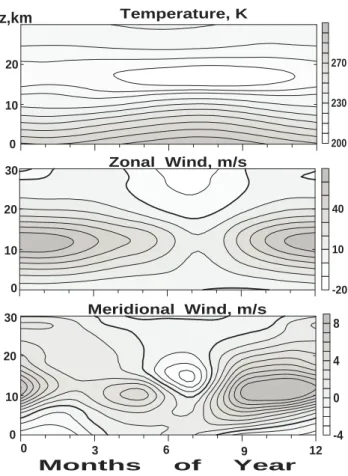
200 230 270 -20 10 40 -4 0 4 8 Temperature, K Zonal Wind, m/s Meridional Wind, m/s 0 3 6 9 12 Months of Year 0 10 20 z,km 0 10 20 30 0 10 20 30

Fig. 2. Background temperature (top), and zonal (middle) and meridional (bottom) wind velocities at Shigaraki, Japan.

Additional IGW generation may be produced by mesoscale meteorological and irregular motions, which pro-duce mesoscale turbulence in the atmosphere. The main contribution to these IGW nonlinear hydrodynamic sources comes from the nonlinear advective accelerations involved in the hydrodynamic momentum equation (see Drobyazko and Krasilnikov, 1985). Observations of the advective accelera-tions in the troposphere and stratosphere with the Japanese MU radar (see Gavrilov and Fukao, 2001) show their strong dependence on the mean wind velocity, v0. Also, we may expect a dependence of s on N , which may influence the in-ferred intensity of turbulent and convective motions in the atmosphere. Gavrilov and Fukao (1999) expressed S(v0, N ) in Eq. (3) in the form of

S(v0, N ) = S0vn₀/Nq, (4)

where S0, n and q are constants. Equations (2)–(4) are solved here for a set of IGW harmonics representing a sta-tistical ensemble of waves propagating from random IGW sources. The background wind components for altitudes 0– 30 km at Shigaraki, Japan, are presented in Fig. 2. We used the monthly mean temperatures and winds taken from the NCEP/NCAR Reanalysis database and averaged them over the years 1980–2000 and from the MU radar measurements as well (Murayama et al., 1994).

200 250

T

, K

A

lti

tud

e

, km

u

, ms

v

, ms

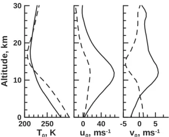
and meridional (right) wind velocities in January (solid lines) and July (dashed lines) at Shigaraki.

For altitudes above 30 km the background temperature and wind were taken from the MSISE-90 and HWM-93 mod-els (Hedin, 1991; Hedin et al., 1996) for different months of the year. Equation (2) contains the rate of IGW dissipation

Nd, due to turbulent and molecular viscosity and heat

con-duction, ion drag, and radiative heat exchange. These char-acteristics, as well as coefficients of turbulent viscosity and heat conduction and dissipation of IGW harmonics at crit-ical and reflection levels, are calculated here, as described by Gavrilov and Fukao (1999). The influence of the criti-cal layers leads, in the model, to stronger dissipation of IGW harmonics propagating in the direction of the mean wind and to the predominance of waves propagating in the opposite direction (Gavrilov, 1997). Such IGW filtering provides, in the model, the wave accelerations of the mean flow directed mainly opposite to the direction of the strato-mesospheric winds in the middle atmosphere (Gavrilov, 1997), which is consistent with recent views (Fritts and Alexander, 2003).

Except for IGW characteristics, the numerical model al-lows ones to estimate turbulent diffusivities caused by break-ing IGWs. We use the method of calculatbreak-ing the turbulent diffusivities within zones of convective and dynamical insta-bilities caused by saturated and unsaturated IGWs developed by Gavrilov and Yudin (1992). The method is based on the closure of spectral turbulent equations using a semiempirical hypothesis for the spectral characteristics of turbulence.

The model has been validated previously by a compari-son of the calculated average wave characteristics with the results of radar observations of the IGW climatology in the middle and upper atmosphere. The numerical model repro-duces different types of seasonal variations of IGW intensity (see Gavrilov and Fukao, 1999), which have the winter max-imum and summer minmax-imum in the upper troposphere and stratosphere, and the solstice maxima and equinox minima in the mesosphere (see Murayama et al., 1994). Gavrilov et

al. (2003) and Gavrilov and Jacobi (2004) applied the numer-ical model for the interpretation of seasonal variations of the wind and ionospheric drift velocity variances observed at al-titudes of 70–110 km with MF radar at Hawaii and with the D1 reflection method at Collm, Germany. The model repro-duces a transition from the solstice maxima of the velocity variances observed near 70–80 km km to the equinox max-ima at higher altitudes.

2.3 Results of numerical simulation

In this study the numerical model involving Eqs. (2)–(4) was run for the background atmosphere representing differ-ent months of the year at the location of the MU radar (see Fig. 2). The numerical methods are further described by Gavrilov (1990). The vertical integration step is of 250 m. The equations were solved for a set of 50×50×12 IGW har-monics, where the multipliers denote the numbers of wave frequencies, horizontal phase speeds and azimuths, respec-tively. The IGW parameters cover the frequency ranges of

σ ∼6×10−4−6×10−3 rad s−1, horizontal phase speeds of c ∼3–100 m/s−1 and azimuths of ϕ∼0◦−360◦. The first two grids were logarithmically spaced (proportional to ln σ , and ln c) within the specified intervals. The values of the constants determining the spectral distributions of the wave sources in the model are the same as those used by Gavrilov and Jacobi (2004). Parameters of the model were chosen to provide IGW power spectral slopes of σ−5/3 and m−3 at large σ and m, corresponding to some observations and theoretical studies (VanZandt, 1982). The parameters were chosen to give the best fit of the calculated results to ob-servations (see below). Gavrilov and Fukao (1999) showed that this model can reproduce realistic seasonal variations of IGW intensity in the troposphere and mesosphere with n=2 in Eq. (4). A strong dependence of the intensity of wave sources on the mean wind in the tropo-stratosphere is con-firmed by recent MU radar measurements of nonlinear ad-vective accelerations (Gavrilov and Fukao, 2001). Therefore, in Eq. (4) we use the values of n=2, S0=10−5m−1s−2 and q=2.

In this study, we calculated vertical profiles of the turbu-lent diffusion coefficient produced by a spectrum of break-ing IGWs. Specifically, we studied the influence of the sharp changes in the vertical temperature gradient in the changes of the conditions of IGW propagation, increasing their destruc-tion and forming a maximum of the turbulent diffusivity near the tropopause. The mean profiles of wind and temperature are specified for the geographic coordinates of the observa-tion site Shigaraki in Japan, from which we have the MU radar data. Figure 3 shows the vertical profiles of background temperature and wind in January and July.

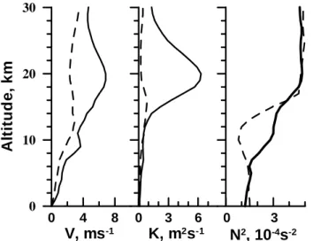
Figure 4 represents the corresponding calculated standard deviations of wind velocity produced by a spectrum of IGWs in the ranges of periods 0.3–6 h and horizontal phase speeds 3–60 m/s and of the coefficient of turbulent diffusion pro-duced by breaking IGWs. One can see that the IGW inten-sity and the turbulent diffusivity have main maxima at

alti-N. M. Gavrilov and S. Fukao: Numerical and the MU radar estimations 3893 0 4 8

V, ms

A

lti

tud

e

, km

K, m

_s

_N

_{, 10}

_s

Fig. 4. Calculated vertical profiles of IGW horizontal velocity

stan-dard deviation (left), turbulent viscosity (middle) and Brunt-V¨ais¨al¨a frequency squared (right) for January (solid lines) and July (dashed lines) at Shigaraki.

tudes 15–20 km, corresponding to the regions with a sharp increase, and maxima of temperature gradient and Brunt-V¨ais¨al¨a frequency in the right plot of Fig. 4. The January temperature profile has two regions of clear changes in verti-cal temperature gradient and Brunt-V¨ais¨al¨a frequency: at al-titudes 9–10 km and 17–19 km (see Figs. 3 and 4). Therefore, one can see a local maximum of IGW amplitudes and turbu-lent viscosity at altitudes 9–10 km in the left plot of Fig. 3. A reason for maxima of IGW amplitudes and turbulent vis-cosity in our model is mainly due to a sharp increase in the Brunt-V¨ais¨al¨a frequency in the tropopause region. This leads to an increase in IGW amplitudes (see Sect. 2.1), wave in-stability and generation of stronger turbulence in our model. The stronger turbulence increases IGW dissipation; there-fore, wave momentum flux and amplitudes become smaller at higher altitudes in Fig. 4. This forms a layer of increased IGW amplitude and turbulent viscosity in the tropopause re-gion in Fig. 4.

Calculated seasonal-altitude distributions of wind vari-ances produced by the IGW ensemble are shown in Fig. 5. One can see substantial seasonal variations with maximum values in winter and the minimum in summer. This maxi-mum occurs just above the tropo-stratospheric jet stream and near the tropopause located at altitudes 15–18 km, depending on the season in Fig. 2. Corresponding distributions of tur-bulent viscosities produced by breaking IGWs are shown in Fig. 6. They also have a maximum in winter and a minimum in summer at altitudes 15–20 km. In summer, the maxima of IGW variances and turbulent viscosity in Figs. 4 and 5 are lower that those in winter. The measurements of IGW inten-sity and turbulent viscointen-sity with the MU radar at Shigaraki also show their maxima near the tropopause (Murayama et al., 1994; Fukao et al., 1994) and with larger values in win-ter than in summer. Our calculated values correspond well

0 3 6 0 3 6 0 3 6 Total r.m.s. Amplitude, m/s Zonal r.m.s. Amplitude, m/s Meridional r.m.s. Amplitude, m/s 0 3 6 9 12 Months of Year 0 10 20 z,km 0 10 20 30 0 10 30 20

Fig. 5. Calculated seasonal distributions of total (top), zonal

(mid-dle) and meridional (bottom) wind standard deviations produced by IGW spectrum.

enough to the measured ones as further discussed in Sect. 3 below.

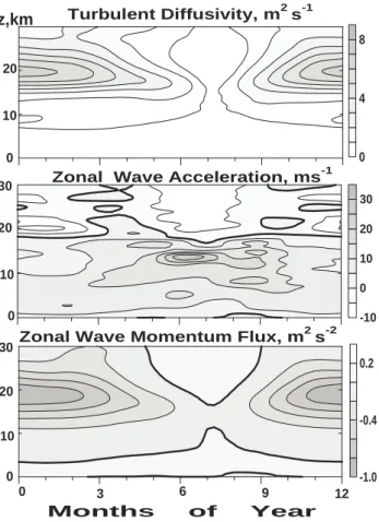
Our numerical model allows us to also calculate such im-portant characteristics as wave momentum flux and acceler-ation of the mean flow produced by dissipating IGWs, which are shown in Fig. 6. These characteristics are important for estimating the IGW influence of atmospheric general circu-lation. One can see that the wave accelerations are mainly positive below the altitudes of 15–16 km, and are negative above these altitudes. In our model, positive zonal wave ac-celerations are created by IGW harmonics propagating east-wards. They may dissipate at critical layers within tropo-stratospheric jet streams and lose their energy there. Nega-tive zonal wave accelerations at larger altitudes are produced by IGWs propagating westward. They do not meet critical levels inside the tropo-stratospheric jet stream, have larger amplitudes, become unstable and produce larger turbulence and wave accelerations at higher altitudes, than the eastward propagating IGWs.

2.4 Estimating vertical ozone fluxes

The presence of turbulence in the atmosphere produces the mixing of atmospheric gases.

0 4 8 -10 0 10 20 30 -1.0 -0.4 0.2 Turbulent Diffusivity, m2s-1

Zonal Wave Acceleration, ms-1

Zonal Wave Momentum Flux, m2s-2

0 3 6 9 12 Months of Year 0 10 20 z,km 0 10 20 30 0 10 20 30

Fig. 6. Calculated distributions of turbulent viscosity (top), wave

acceleration of the mean flow (middle) and vertical component of zonal wave momentum flux (bottom). Solid lines correspond to zero values.

Possible increase in IGW intensity and turbulence near the tropopause described above may lead, in particular, to an in-crease in fluxes of atmospheric admixtures from the tropo-sphere to the stratotropo-sphere or back, depending on the vertical distribution of the particular admixture. In particular, tur-bulence may influence descending of ozone from the strato-sphere to the tropostrato-sphere. The vertical flux of an admixture can be described by the following formula:

F = −Knc∂(ln c)/∂z, (5)

where K is the turbulent diffusion coefficient; n is the num-ber density of the atmosphere; c is the mixing ratio of the considered admixture. Using the values of c for the alti-tudes of 12–17 km from the model of vertical ozone profile (Zuev and Komarov, 1986) and the values of K∼1–10 m2/s shown in Figs. 3 and 5, we may obtain the estimate F ∼(1– 10)×1014m−2s−1.

The main, recently assumed, global-scale mechanism of penetration of the stratospheric ozone into the troposphere is its transport by the general atmospheric circulation from equatorial latitudes and descending of the air in the middle latitudes (Holton, 1990). The mean downward ozone flux due to the circulation transport is estimated to be about F

∼7×1014m−2s−1(Ebel et al., 1993), while the estimations of

tropospheric ozone require the fluxes of stratospheric ozone to be of the order of (4–8)×1014m−2_s−1_{(e.g. Crutzen, 1988).} Comparison of these values with the estimations of the ozone diffusion flux obtained above show that these values may be-come comparable. Therefore, in some regions and times tur-bulence generation by gravity waves near the tropopause may produce noticeable transport of ozone from the stratosphere to the troposphere.

One can estimate the characteristic time scale required for the transport of all stratospheric ozone into the troposphere (in the absence of its sources): τ ∼ q/F , where q is the to-tal ozone content in the atmospheric column above the al-titude considered. The estimates of Kdescribed above, to-gether with the model of vertical ozone distribution (Zuev and Komarov, 1986), lead to the values of τ ∼0,3–3 days. These values show that the changes in IGW intensity and turbulence near the tropopause may lead, relatively fast, to the changes in the stratospheric ozone concentration and to a shift in the photochemical equilibrium.

3 Comparison with measurements and discussion

The numerical model used in this study is a simple, one-dimension model of IGW propagation. More realistic three-dimension simulations of turbulent mixing in the unstable jet streams near the tropopause (Joseph et al., 2003, 2004) also revealed maxima of turbulent characteristics in the re-gions with a sharp increase in the Brunt-V¨ais¨al¨a frequency in the tropopause region. This three-dimensional model does not include breaking IGWs and involves wind shears as the main source of turbulent energy inside the jet stream. Possi-ble growing of IGW amplitudes and wave breaking discussed above may produce additional turbulence generation within and above the tropopause jet stream.

It is interesting to compare the results of numerical calcu-lations described in the previous section with the results of the measurements with the MU radar operating in Shigaraki (35◦N, 136◦E) since the year 1984. Numerous studies of IGWs and turbulent diffusivity in the tropo-stratosphere were made with this radar (Fukao et al., 1994; Murayama et al., 1994; Kurosaki et al., 1996; etc.) These studies showed that the mean value and variance of wind velocity, as well as turbulent diffusivity, have strong seasonal variations near the tropopause, with the maxima in winter and minima in summer. The standard deviations of variations of zonal and meridional wind components with time scales of 5 min– 21 h are about 3.5–4 m/s in January and 2–2.5 m/s in July at heights of 15–17 km (Murayama et al., 1994). Measured mean vertical profiles of kinetic energy of wind variations with periods of 5 min–2 h have the main maxima at altitudes 11–13 km in winter and 13–14 km in summer (Murayama et al., 1994). They correspond to the locations of the maxi-mum of tropo-stratospheric jet streams in different seasons. In many cases individual profiles of the kinetic energy have the secondary maxima at altitudes 15–20 km (Murayama et al., 1994).

N. M. Gavrilov and S. Fukao: Numerical and the MU radar estimations 3895 In comparing these experimental results with our

numeri-cal modelling one should keep in mind that the numeri-calculations of Sect. 3 refer to propagating IGWs, but several reasons for the wind variability in the tropo-stratosphere may occur. One of them may be the generation of turbulence due to wind shears inside the jet stream (Joseph et al., 2003, 2004). An-other reason could be the generation of mesoscale irregulari-ties by instabiliirregulari-ties within the tropo-stratospheric, jet stream. These irregularities could be more intensive in winter, when the speed of the jet is higher over Shigaraki. Such irregulari-ties are located mainly inside the jet stream, producing some sort of mesoscale turbulence, which could be much stronger, than propagating IGWs located there. Due to nonlinear in-teractions, this quasi-two-dimensional mesoscale turbulence may generate gravity waves, which can propagate upwards. Gavrilov et al. (1999) used 9-beam MU radar measurements for estimating mesoscale variability of nonlinear advective accelerations responsible for Lighthill-type IGW generation. They showed that these accelerations are largest at altitudes of the tropo-stratospheric jet stream maxima. IGWs gener-ating by nonlinear interactions of this mesoscale turbulence inside the jet stream and propagating from other tropospheric sources could be the third reason for observed wind variabil-ity. These waves could be relatively weak compared with irregularities inside the tropo-stratospheric jet, but may be-come noticeable at higher altitudes, where their amplitudes grow. IGWs propagating from below may form secondary maxima of wind variability at altitudes 15–20 km observed in many individual monthly profiles by Murayama et al. (1994) and expected from the numerical modelling of Sect. 2.

The question is how well do these observed secondary maxima of wind variability correspond to the observed tropopause heights. Numerical simulation in Sect. 2 was made for climatological mean temperature and wind dis-tributions, which are smooth with clear temperature min-ima. In real experiments the tropopause height is not very stable. Mesoscale disturbances and enhancing IGWs may superimpose to the mean temperature profile shifting the main temperature minimum and forming additional minima. One should expect that these dynamical disturbances of the tropopause could be larger in winter, when mesoscale distur-bances within the jet stream and IGW activity are larger. In reality, Murayama et al. (1994) observed larger variability of the tropopause height over Shigaraki in winter. In many cases temperature minima appeared at altitudes 9–10 km within the tropo-stratospheric jet. Climatologically speaking, this cor-responds to a clear change in the vertical temperature gra-dient at altitudes 9–10 km in January, in Fig. 3. Therefore, the maxima of propagating IGWs caused by a sharp increase in the Brunt-V¨ais¨al¨a frequency near such low temperature minima (see Fig. 4) may overlap with the wind variability produced by the jet streams instabilities. Also, substantial al-titude variability of the tropopause creates difficulties in the localization of corresponding IGW maxima in winter.

In summer, the tropopause heights over Shigaraki are more stable and vary between 15 and 17 km (Murayama et al., 1994). As a result, many vertical profiles of kinetic energy

of wind variations with periods of 5 min–2 h in Fig. 8 of the paper by Murayama et al. (1994) have secondary maxima at altitudes 17–19 km, just above the tropopause. This broadens the maximum at the mean summer profile of the kinetic en-ergy in the same figure, which expands from 13 up to 18 km (see Murayama et al., 1994). This shows that the increase in the Brunt-V¨ais¨al¨a frequency near the tropopause may re-ally influence IGW propagation and may increase their am-plitudes.

Fukao et al. (1994) studied seasonal variations of eddy dif-fusivity, K, measured by the MU radar, using the Doppler velocity spectral width method. They found broad distri-butions of K(z) with maxima between altitudes 12–14 km and median values of K>1 m2/s up to altitudes 16–20 km, depending on season. The winter median values of K are generally larger than those in summer, although high tropo-stratospheric jet velocity in winter produces large broadening of the Doppler velocity spectrum and makes measurements of K almost impossible. Kurosaki et al. (1996) obtained an-nual mean vertical profiles of K for the years 1986–1992. They found median values of K up to 6 m2/s at altitudes 10– 14 km and K>1 m2/s up to altitudes 17–18 km. Therefore, the influence of the increase of the Brunt-V¨ais¨al¨a frequency on the increasing of IGW activity near the tropopause may slow down the decrease in K above tropo-stratospheric jet stream and provides substantial turbulent diffusivities near the tropopause.

Gavrilov et al. (2004) estimated turbulent diffusivities,

K, and vertical turbulent ozone fluxes, F , in the tropo-stratosphere from simultaneous measurements with the MU radar and ozonesondes at Shigaraki, Japan, in April 1998. They obtained local maximum values of K up to 6– 10 m2/s−1 _{and F up to −(30–40)×10}14−2_s−1_{, at altitudes,} 8–14 km in the tropopause region. Both K and F have com-plicated intermittent vertical structures with multiple local maxima and minima of K and F . Therefore, further study is required for obtaining climatological mean values of K and F in different locations and seasons.

Pavelin et al. (2002) and Whiteway et al. (2003) reported about smaller values of K∼1–2 m2/s−1near the tropopause, which were measured with an aircraft over England. One reason for K differences between Japan and Europe may be much larger speeds of the jet stream over Japan. According to Murayama et al. (1994) the speed of the jet stream over Shigaraki in January may reach up to 90–100 m/s−1, which is much larger than the speeds of the jet streams observed over Europe (Pavelin et al., 2002; Whiteway et al., 2003). Also, the MU radar is located in the mountain region, while aircraft measurements of Pavelin et al. (2002) and Whiteway et al. (2003) were made over plane surface. Therefore, differ-ences in orography and dynamical activity of the atmosphere may lead to local differences of IGW intensity, turbulence and ozone fluxes over different regions.

Another reason for the discrepancies between aircraft and MST radar measurements of K may be the possible over-estimation of K measured by the radars. There are several reasons which may cause such an overestimation.

One of them is the Doppler spectrum broadening caused by the influence of the mean wind and its vertical gradient (see Hocking, 1985). Other formulae for the Doppler spec-tral width correction for the broadening were developed by Nastrom (1997). VanZandt et al. (2002) developed a dual-beamwidth method for estimating the Doppler spectral width of MST radars. The authors showed that after correction their method may give smaller values of the spectral width than the one-beamwidth method used by Fukao et al. (1994) and Kurosaki et al. (1996).

Another problem for the MST radar measurements of tur-bulence is connected with the formulae used for estimating effective turbulent diffusivity from measured Doppler spec-trum width. Hocking (1999) emphasised the role of spa-tial and temporal intermittency, which may be produced by IGWs creating regions of instability separated by regions of stability. Dewan (1981) and Woodman and Rastogi (1984) suggested that the random occurrence of turbulent layers may produce a random process of intermittent diffusion and an effective turbulent diffusivity of this ensemble should be in-troduced. Fritts and Dunkerton (1985) and Gavrilov and Yudin (1992) showed that the intermittency may lead to the difference in diffusivity of momentum and heat, causing an increase in the effective Prandtl number from 1 up to 3. High resolution balloon temperature measurements showed that turbulence in the tropo-stratosphere most frequently oc-cur within relatively thin unstable layers (Luce et al., 2002). Therefore, turbulent transport of a particle may occurs only within this layer until it dies out. Then the particle remains nearly stationary because of negligible molecular diffusion. Later in time, another turbulent layer forms around the par-ticle and further transport over the depth of the layer is pos-sible. Therefore, climatologically, speaking, the transport of atmospheric species may depend on an effective diffusivity averaged over substantial time intervals rather than on local turbulent diffusivities measured at a particular experiment. Taking account of this as well as other aspects of the prob-lem, Hocking (1999) supposed that the relation between tur-bulent diffusivity and energy dissipation rate measured by MST radars may not be so simple as it is usually assumed.

Resulting effective diffusivity caused by random intermit-tent diffusion might be smaller than local diffusivities mea-sured by radar within turbulent regions. Estimations of ver-tical ozone fluxes from the stratosphere to the troposphere are made in Sect. 2.4 for values of K∼1–10 m2/s observed with the MU radar. A comparison of these estimations with the fluxes caused by atmospheric general circulation (see Sect. 2.4) shows that even for values of K up to several times smaller than those used in Sect. 2.4, turbulent ozone flux could be a noticeable addition to conventional transport of ozone due to circulation from the tropics to the middle lati-tudes. Therefore, improvement of the methods of MST radar studies of atmospheric turbulence and atmospheric admix-tures transport through the tropopause are very urgent and important.

Estimations of the time scales of stratospheric ozone changes due to turbulent diffusion, τ , in Sect. 2.4, show that

the variability of turbulence activity near the tropopause due to meteorological processes and local conditions may result in noticeable changes in stratospheric, tropospheric and to-tal ozone. Satellite observations show toto-tal ozone variability related to tropical cyclones (Nerushev, 1996). One of the mechanisms for such relations could be an increase in the instability and turbulence, within a cyclone, which leads to more active ozone transport from the stratosphere into the troposphere. Local enhancements of IGW intensity and tur-bulence due to their orographic excitation, may lead to the changes in total ozone over the mountain regions. This may explain, for example, the observed anomalies of total ozone over the mountain regions (Kazimirovsky and Matafonov, 1998).

4 Conclusions

A numerical simulation performed in this paper shows that a sharp change in the vertical temperature gradient and the Brunt-V¨ais¨al¨a frequency near the tropopause may produce an increase in amplitudes of IGWs propagating upward from the troposphere, wave breaking and generation of stronger turbulence. This may make the middle latitude tropopause more transparent for the transport of admixtures between the troposphere and the stratosphere. An increase in the turbu-lent diffusivities at altitudes near and above the tropopause is usually observed with the MU radar in Shigaraki, Japan (35◦N, 136◦E). Turbulent diffusivity calculated numerically and measured with the MU radar is of 1–10 m2/s in the tropopause region in different seasons. This leads to the esti-mation of vertical ozone flux from the stratosphere to the tro-posphere of the order of (1–10)×1014m−2/s−1, which may become comparable with ozone downward fluxes with the general atmospheric circulation. Therefore, local enhance-ments of IGW intensity and turbulence at tropospheric al-titudes over the mountains, due to their orographic excita-tion and due to other wave sources, may lead to the changes in the tropospheric ozone and the total ozone over different regions. Improving methods of MST radar evaluations of turbulent diffusivity and simultaneous ozonosonde measure-ments are highly important for better estimating the ozone turbulent transport through the tropopause.

Acknowledgements. This study was partly supported by the

Rus-sian Basic Research Foundation and by the International Science and Technology Center. The MU radar belongs to and is operated by the Center for Atmospheric and Space Research of Kyoto Uni-versity.

Topical Editor U.-P. Hoppe thanks S. J. Reid and another referee for their help in evaluating this paper.

References

Alexander, M. J. and Holton, J. R.: A model study of zonal forc-ing in the equatorial stratosphere by convectively induced gravity waves, J. Atmos. Sci., 54, 408–419, 1997.

N. M. Gavrilov and S. Fukao: Numerical and the MU radar estimations 3897

Andrews, D. G., Holton, J. R., and Leovy, C. B.: Middle atmo-sphere dynamics, Academic Press, New York, 1987.

Birner, T., Dornbrack, A., and Schuman, U.: How sharp is the tropopause at midlatitudes?, Geophys. Res. Lett., 29(14), doi10.1029/2002GL015142, 2002.

Crutzen, P. J.: Tropospheric ozone: An overview, In I. S. A Isaken (ed.), Tropospheric Ozone, D. Reidel Publ. Company, Dordrecht, 3–32, 1988.

Dameris, M.: Tropopause, Enciclopedia of Atmospheric Sciences, Ed. by J. R. Holton, Academic Press, Amsterdam-New York– Tokyo, 2346–2348, 2003.

Dewan, E. M.: Turbulent vertical transport due to thin intermitten mixing layers in the atmosphere and other stable fluids, Science, 211, 1041–1042, 1981.

Drobyazko, I. N. and Krasilnikov, V. N.: Acoustic-gravity wave generation by atmospheric turbulence, Radiophysics, Izvestia VUZov of USSR, 28, 1357–1365, 1985.

Ebel, A., Elbern, H., and Oberreuter, A.: Stratosphere-troposphere air mass exchange and cross-tropopause fluxes of ozone. In Cou-pling processes in the lower and middle atmosphere, eds. Thrane, E. V. et al., Kluner, Dordrecht, 49–65, 1993.

Fritts, D. C. and Dunkerton, T. J.: Fluxes of heat and constituents due to convectively unstable gravity waves, J. Atmos. Sci., 42, 549–556, 1985.

Fritts, D. C. and VanZandt, T. E.: Effects of Doppler shifting on the frequency spectra of atmospheric gravity waves, J. Geophys. Res., 92, 9723–9732, 1987.

Fritts, D. C. and Alexander, M. J.: A review of gravity wave dy-namics and effects in the middle atmosphere, Rev. Geophys., 41, 2003.

Fukao, S., Yamanaka, M. D., Ao, N., Hocking, W. K., Sato, T., Yamamoto, M., Nakamura, T., Tsuda, T., and Kato, S.: Seasonal variability of vertical eddy diffusivity in the middle atmosphere, 1. Tree-year observations by the middle and upper atmosphere radar, J. Geophys. Res., 99, 18 973–18 987, 1994.

Gardner, C. S., Tao, X., and Papen, G. C.: Simultaneous lidar obser-vations of vertical wind, temperature and density profiles in the upper mesosphere: Evidence for nonseparability of atmospheric perturbation spectra, Geophys. Res. Lett., 22, 2877–2880, 1995. Gavrilov, N. M.: Parameterization of accelerations and heat flux divergences produced by internal gravity waves in the middle at-mosphere. J. Atmos. Terr. Phys., 52, 707–713, 1990.

Gavrilov, N. M.: Parameterization of momentum and energy depo-sitions from gravity waves generated by tropospheric hydrody-namic sources. Ann. Geophys., 15, 1570–1580, 1997.

Gavrilov, N. M. and Fukao, S.: A comparison of seasonal variations of gravity wave intensity observed with the middle and upper atmosphere radar with a theoretical model. J. Atmos. Sci., 56, 3485–3494, 1999.

Gavrilov, N. M. and Fukao, S.: Hydrodynamic tropospheric wave sources and their role in gravity wave climatology of the upper atmosphere from the MU radar observations, J. Atmos. Solar-Terr. Phys., 63, 931–943, 2001.

Gavrilov, N. M., Fukao, S., and Hashiguchi, H.: Multi-beam MU radar measurements of advective accelerations in the atmo-sphere, Geophys. Res. Lett., 26, 315–318, 1999.

Gavrilov N. M., Fukao, S., Hashiguchi, H., Kita, K., Sato, K., Tomikawa, Y. and Fujiwara, M.: Study of Atmospheric Ozone and Turbulence From Combined MU Radar and Ozonesonde Measurements in Shigaraki, Japan., Proc. XX Quadrennial Ozone Symp., Kos, Greece, 1–8 June, 41–42, 2004.

Gavrilov, N. M. and Jacobi, Ch.: A study of seasonal variations of

gravity wave intensity in the lower thermosphere using LF D1 wind observations and a numerical model, Ann. Geophys., 22, 35–45, 2004.

Gavrilov, N. M., Riggin, D. M., and Fritts, D. C.: Medium-frequency radar studies of gravity-wave seasonal variations over Hawaii (22◦N, 160◦W), J. Geophys. Res., 108, 4655, 10.1029/2002JD003131, 2003.

Gavrilov, N. M. and Yudin, V. A.: Model for Coefficients of Turbu-lence and Effective Prandtl Number Produced by Breaking Grav-ity Waves in the upper Atmosphere, J. Geophys. Res., 97, 7619– 7624, 1992.

Hedin, A. E.: Neutral atmosphere empirical model from the surface to lower exosphere MSISE-90, Extension of the MSIS thermo-sphere model into the middle and lower atmothermo-sphere, J. Geophys. Res., 96, 1159–1172, 1991.

Hedin, A. E., Fleming, E. L., Manson, A. H., Schmidlin, F. J., Av-ery, S. K., Clark, R. R., Franke, S. J., Fraser, G. J., Tsuda, T., Vial, F., and Vincent, R. A.: Empirical model for the upper, mid-dle and lower atmosphere, J. Atmos. Terr. Phys., 58, 1421–1447, 1996.

Hocking, W. K.: Measurements of turbulent energy dissipation rate in the middle atmosphere by radar techniques: a review, Radio Sci., 20, 1403–1422, 1985.

Hocking, W. K.: The dynamical parameters of turbulence theory as they apply to middle atmosphere studies, Earth Planet. Sci., 51, 525–541, 1999.

Holton, J. R.: On the global exchange of mass between the strato-sphere and tropostrato-sphere, J. Atmos. Sci., 47, 392–395, 1990. Joseph, B., Mahalov, A., Nikolaenko, B., and Tse, K. L.: High

reso-lution DNS of jet stream generated tropopausal turbulence, Geo-phys. Res. Lett., 30, 1525, doi:10.1029/2003GL017252, 2003. Joseph, B., Mahalov, A., Nikolaenko, B., and Tse, K. L.: Variability

of turbulence and its outer scales in a model tropopause jet, J. Atmos. Sci., 61, 621–643, 2004.

Kazimirovsky, E. S. and Matafonov G. K.: Continental scale and orographic structures in the global distribution of the total ozone, J. Atmos. Solar-Terr. Phys., 60, 993–996, 1998.

Kurosaki, S., Yamanaka, M. D., Hashiguchi, H., Sato, T, and Fukao, S.: Vertical eddy diffusivity in the lower and middle atmosphere: a climatology based on the MU radar observations during 1986– 1992, J. Atmos. Terr. Phys., 58, 727–734, 1996.

Lamarque J. F. and P. Hess. Stratosphere-troposphere exchange: Local processes, Enciclopedia of Atmospheric Sciences, Ed. By. J. R. Holton, Academic Press, Amsterdam – New York – Tokyo, 2143–2150, 2003.

Lighthill, M. J.: On sound generated aerodynamically, 1. General theory, Proc. Roy. Soc. London, A211, 564–587, 1952. Lighthill, M. J.: Waves in fluids, Cambridge Univ. Press, 1978. Luce, H., Fukao, S., Dalaudier, F., and Crochet, M.: Strong Mixing

Events Observed near the Tropopause with the MU Radar and High-Resolution Balloon Techniques, J. Atmos. Sci., 59, 2885– 2896, 2002.

Monin, A. S. and Yaglom, A. M.: Statistical fluid mechanics, 1, MIT Press, Cambridge, MA. 1971.

Murayama, Y., Tsuda, T., and Fukao, S.: Seasonal variations of gravity wave activity in the lower atmosphere observed with the MU radar, J. Geophys. Res., 99, 23 057–23 069, 1994.

Nastrom, G. D.: Doppler radar spectral width broadening due to beamwidth and wind shear, Ann. Geophys., 15, 786–796, 1997. Nerushev, A. F.: Tropical cyclone influence on the ozonosphere,

Izv. Acad. Sci. USSR Atmos. Oceanic Phys., 31, 40–46, 1996. Pavelin, E., Whiteway, J. A., and Vaughan, G.: Observation of

grav-ity wave generation and breaking in the lowermost stratosphere, J. Geophys. Res., 106, 5173–5179, 2001.

Pavelin, E., Whiteway, J., Busen, R., and Hacker, J.: Air-borne observations of turbulence, mixing and gravity waves in the tropopause region: J. Geophys. Res., 107(D10), 4084, doi:10.1029/2001JD000775, 2002a.

Pavelin, E. and Whiteway, J.: Gravity wave interactions around the jet stream, Geophys. Res. Lett., 29(21), 2024, doi:10.1029/2002GL015783, 2002.

Stein, R. S.: Generation of acoustic and gravity waves by turbulence in an isothermal stratified atmosphere, Solar Phys., 2, 285–432, 1967.

VanZandt, T. E.: A universal spectrum of buoyancy waves in the atmosphere, Geophys. Res. Lett., 9, 575–578, 1982.

VanZandt, T. E., Nastrom, G. D., Furumoto, J., Tsuda, T., and Clark, W. L.: A dual-beamwidth radar method for measuring atmo-spheric turbulent kinetic energy, Geophys. Res. Lett., 29, 1572, 10.1029/2001GL014283, 2002.

Whiteway, J. A., Pavelin, E. G., Busen, R., Hacker, J., and Vosper, S.: Airborn measurements of gravity wave breaking at the tropopause, Geophys. Res. Lett., 30(20), doi:10.1029/2003GL018207, 2003.

Woodman, R. F. and Rastogi P. K.: Evaluation of effective eddy diffusive coefficients using radar observations of turbulence in the stratosphere, Geophys. Res. Lett., 11, 243–246, 1984. Zuev, V. E. and Komarov V. S.: Statistical models of temperature

and gas components of the atmosphere, Hydrometeoizdat Press, Leningrad, 1986.