HAL Id: hal-00317210
https://hal.archives-ouvertes.fr/hal-00317210
Submitted on 1 Jan 2004
HAL is a multi-disciplinary open access
archive for the deposit and dissemination of
sci-entific research documents, whether they are
pub-lished or not. The documents may come from
teaching and research institutions in France or
abroad, or from public or private research centers.
L’archive ouverte pluridisciplinaire HAL, est
destinée au dépôt et à la diffusion de documents
scientifiques de niveau recherche, publiés ou non,
émanant des établissements d’enseignement et de
recherche français ou étrangers, des laboratoires
publics ou privés.
Origins of the semiannual variation of geomagnetic
activity in 1954 and 1996
E. W. Cliver, L. Svalgaard, A. G. Ling
To cite this version:
E. W. Cliver, L. Svalgaard, A. G. Ling. Origins of the semiannual variation of geomagnetic activity
in 1954 and 1996. Annales Geophysicae, European Geosciences Union, 2004, 22 (1), pp.93-100.
�hal-00317210�
Annales Geophysicae (2004) 22: 93–100 © European Geosciences Union 2004
Annales
Geophysicae
Origins of the semiannual variation of geomagnetic activity in 1954
and 1996
E. W. Cliver1, L. Svalgaard2, and A. G. Ling3
1Space Vehicles Directorate, Air Force Research Laboratory, Hanscom AFB, MA 01731, USA 2Easy Tool Kit, Inc., Houston, TX 77055, USA
3Radex, Inc., Bedford, MA 01730, USA
Received: 4 February 2003 – Revised: 12 May 2003 – Accepted: 27 May 2003 – Published: 1 January 2004
Abstract. We investigate the cause of the unusually strong
semiannual variation of geomagnetic activity observed in the solar minimum years of 1954 and 1996. For 1996 we separate the contributions of the three classical modulation mechanisms (axial, equinoctial, and Russell-McPherron) to the six-month wave in the aam index and find that all three
contribute about equally. This is in contrast to the longer run of geomagnetic activity (1868–1998) over which the equinoctial effect accounts for ∼70% of the semiannual vari-ation. For both 1954 and 1996, we show that the Russell-McPherron effect was enhanced by the Rosenberg-Coleman effect (an axial polarity effect) which increased the amount of the negative (toward Sun) [positive (away from Sun)] polar-ity field observed during the first [second] half of the year; such fields yield a southward component in GSM coordi-nates. Because this favourable condition occurs only for al-ternate solar cycles, the marked semiannual variation in 1954 and 1996 is a manifestation of the 22-year cycle of geomag-netic activity. The 11-year evolution of the heliospheric cur-rent sheet (HCS) also contributes to the strong six-month wave during these years. At solar minimum, the streamer belt at the base of the HCS is located near the solar equa-tor, permitting easier access to high speed streams from po-lar coronal holes when the Earth is at its highest heliographic latitudes in March and September. Such an axial variation in solar wind speed was observed for 1996 and is inferred for 1954.
Key words. Magnetosphere (solar wind – magnetosphere
interactions; storms and substorms)
1 Introduction
The cause of the semiannual variation of geomagnetic activ-ity, characterized by stronger and more frequent storms in spring/fall vs. summer/winter, is a long-standing question (e.g. Sabine, 1856) for which three mechanisms have been Correspondence to: E. W. Cliver (cliver@plh.af.mil)
proposed. The equinoctial hypothesis (Bartels, 1925, 1932; McIntosh, 1959; Svalgaard, 1977) is governed by the ψ an-gle between the solar wind flow direction and the Earth’s dipole axis. Under this hypothesis, activity maximizes (for as yet unknown reasons) at the equinoxes when ψ is 90◦. The key angle in the axial hypothesis (Cortie, 1912) is the heliographic latitude of the Earth (BO). In early March
and September the Earth is at its maximum angular distance (∼7◦) from the solar equatorial plane and thus more closely aligned with both the sunspot zones and coronal holes that extend down from the solar poles. In the Russell-McPherron mechanism (Russell and McPherron, 1973), magnetic fields in the solar equatorial plane have a peak southward compo-nent at the Earth in Geocentric Solar Magnetospheric (GSM) coordinates in early April or October, depending on their po-larity.
While all of these mechanisms contribute to the semian-nual variation, their relative contributions have long been a matter of debate (e.g. Mayaud, 1974a; Russell and McPher-ron, 1974). Recently, various authors (Cliver et al., 2000, 2001, 2002; Lyatsky et al., 2001; Temerin and Li, 2002; O’Brien and McPherron, 2002) have argued that the equinoc-tial hypothesis plays a more important role vis-`a-vis the competing axial and (in particular) Russell-McPherron (RM) mechanisms than has previously been thought to be the case. Cliver et al. (2000) and Svalgaard et al. (2002) calculated that, on average, the equinoctial hypothesis accounts for 65– 75% of the amplitude of the six-month wave in the geomag-netic am index.
The present study does not deal with average conditions. Occasionally, the semiannual variation of geomagnetic activ-ity is so pronounced that one can readily identify the equinoc-tial peaks and solstiequinoc-tial valleys in plots of daily averages of geomagnetic indices during the year. The solar minimum years of 1954 and 1996 were two such intervals. In this study we ask why the six-month wave was so prominent during these years. Our analysis is presented in Sect. 2 and the re-sults are discussed in Sect. 3.
94 E. W. Cliver et al.: Origins of the semiannual variation
Fig. 1. Plots of daily values of the aamindex for (a) 1954 and (b) 1996.
2 Analysis
2.1 Selection of years
To identify years with a pronounced semiannual variation, we used the aam index recently introduced by Svalgaard
et al. (2002). The aam index is the aa index1 (Mayaud,
1972, 1980), available from 1868–1998, modified to have the correct universal time variation. We correlated the di-urnal/seasonal matrix (8 × 12; 3 h, 1 month) of aamvalues
for each of the 131 years with the equinoctial angle (ψ ), the Russell-McPherron angle (the angle between the z-axis in the GSM coordinate system and the solar equatorial plane, mea-sured in the y − z (GSM) plane), and the axial angle (BO).
1The aa index is a mid-latitude range index based on maximum excursions of the horizontal (H ) or declination (D) components of the field over a 3-h interval after removing the regular variation (SR). aa is based on two nearly-antipodal stations in England and Australia; because the stations are not exactly antipodal, the UT-dependence is distorted, hence, the correction as described.
Fig. 2. Diurnal/seasonal variation of the aamindex during 1996.
Because of the ∼11◦offset of the Earth’s dipole axis to the rotation axis, both the equinoctial and Russell-McPherron mechanisms produce a Universal Time variation (UT), as well as seasonal variation, while the axial effect has no UT dependence. From 1868–1998, 37 indiviudal years had aam -ψangle correlation coefficients ≥ 0.5, in comparison with 9 such years for BOand only 4 years (≤ −0.5) for the RM
an-gle. We selected for further analysis the only two years that had numeric correlation coefficients ≥ 0.5 in all three in-dices: 1954 (r = 0.66(ψ ); r = −0.50(RM); r = 0.59(BO))
and 1996 (r = 0.70(ψ ); r = −0.51(RM); r = 0.56(BO)).
Our technique thus identified years that had strong semian-nual variations that could be plausibly accounted for in terms of any one, or a combination, of the three classic modulation hypotheses. Figure 1a and b give plots of daily values of aam
for 1954 and 1996, respectively. In both cases, the six-month wave in geomagnetic activity is readily discernible.
2.2 Origins of the semiannual variation of geomagnetic ac-tivity in 1996
2.2.1 ψ-angle normalization
A diurnal/seasonal plot of the aam index for 1996 is given
in Fig. 2. To remove the contribution from the equinoc-tial mechanism, we follow the procedure of Svalgaard et al. (2002) (see also O’Brien and McPherron, 2002) and multiply aam by 0.864 (1 + cos2ψ )2/3 to obtain the ψ
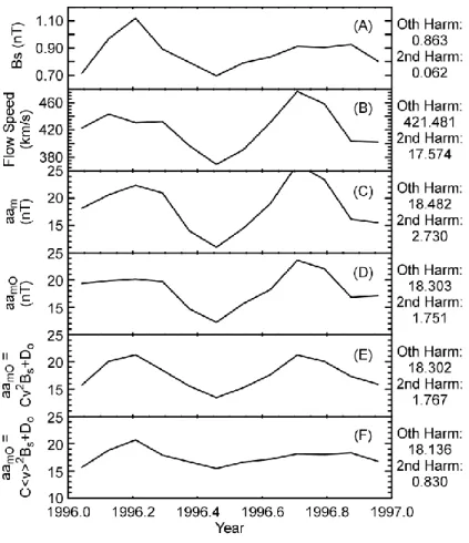
-normalized aam0 index. Figure 3 gives plots of monthly averages of (a) southward magnetic field (BS, in GSM
co-ordinates), (b) solar wind speed (v), (c) the aamindex, and
(d) the aam0index for 1996. An FFT analysis of the aam
and aam0 indices shows that the ψ -normalization removes only ∼35% of the amplitude of the second harmonic (given in the figure) vs. the 65–75% figure obtained by Cliver et al. (2000) and Svalgaard et al. (2002) for the contribution from the equinoctial effect.
E. W. Cliver et al.: Origins of the semiannual variation 95
Fig. 3. Monthly averages for 1996 of (a) southward magnetic field (Bs), (b) solar wind flow speed (v), (c) aam in-dex, (d) “observed” aam0index, (e) cal-culated aam0index (from Eq. 1; C = 7.551 × 10⁻⁵, DO = 6.554), and (f) calculated aam0index with solar wind flow speed (v) held constant at its yearly average of 421km s−1. The average value (0th harmonic) and coefficient of the 2nd harmonic of each parameter are given in the right-hand margin.
2.2.2 Contributions from the Russell-McPherron and axial mechanisms
The semiannual variations of BS(Fig. 3a) and v (Fig. 3b)
in-dicate that both the Russell-McPherron effect and the axial effect contribute to the six-month wave in aam0. To sepa-rate and quantify these contributions, we obtained the fol-lowing relationship between monthly averages of aam0 and solar wind parameters for 1996, assuming the standard func-tional form between these variables deduced by various au-thors (e.g. Feynman and Crooker, 1978)
aam0=7.551 × 10⁻⁵v2BS+6.554 . (1)
Figure 3e shows that aam0(calculated from Eq. 1) has an average value and second harmonic coefficient that are com-parable to those for the observed aam0(Fig. 3d). To obtain Fig. 3f, the value of v was held constant at the 1996 annual average of 421km s−1, thereby removing the axial solar wind speed contribution to the semiannual variation. The remain-ing ∼50% (0.83/1.77) of the semiannual variation of aam0 is attributed to the Russell-McPherron effect. (An essen-tially identical result is obtained by holding BS constant.)
Approximately equal contributions for the axial and Russell-McPherron effects are consistent with correlations of the di-urnal/seasonal matrix of aam0with BO(r = 0.50) and the
RM angle (r = −0.47). Thus, we conclude that for 1996,
all three of the classic modulation mechanisms contributed about equally to the six-month wave in the aamindex.
2.2.3 Causes of the enhanced Russell-McPherron and axial contributions
The Russell-McPherron mechanism assumes that the inter-planetary magnetic field measured at the Earth is equally likely to be pointed inward or outward during the year. For long intervals this is a good assumption, e.g. for the 1963– 2000, we find that BX is positive (negative) 50.4% (49.6%)
of the time. For shorter intervals of time, however, the po-larity mix can deviate from parity. In particular, for peri-ods near solar minimum when the heliospheric current sheet (HCS) lies close to the solar equator, the Earth can find itself preferentially in one polarity or the other for six month in-tervals as it ranges between ∼7◦N and ∼7◦S in heliospheric
latitude. Rosenberg and Coleman (1969) were the first to draw attention to this axial polarity effect. The Rosenberg-Coleman polarity effect is evident in 1996. During this year, the solar wind polarity was biased negative (inward) during the first half of the year and positive (outward) during the second half (Fig. 4), circumstances under which the Russell-McPherron coordinate transformation from Geocentric Solar Equatorial (GSEq) to GSM coordinates yields a southward pointing magnetic field component. In all, the magnetic po-larity at the Earth was favourable for 63% of all hours during
96 E. W. Cliver et al.: Origins of the semiannual variation
Fig. 4. Solar wind magnetic polarity distribution (5-day averages)
at the Earth during 1996. Fields with positive (negative) Bxare di-rected toward (away from) the Sun. The dashed vertical lines indi-cate mimima (favourable polarity cross-over times) for the Russell-McPherron effect. The dashed horizontal lines give average per-centages of the time Bxis positive for intervals bounded by these crossings (the second interval is truncated on 31 December). Note that Bxhas the opposite sign of the solar/solar wind magnetic po-larity.
1996, vs. the ∼50% long-term average, indicating a Russell-McPherron effect that was theoretically ∼25% stronger than usual. Comparison of the coefficients of the second harmon-ics in FFT analyses of Bs for 1996 (0.62) and the interval
1963–2000 (0.38) indicates an actual increase of ∼60%. Figure 5 shows the evolution of the “tilt angle” (Smith and Thomas, 1986) of the HCS during the period from 1990– 2000. The tilt angle is obtained from computed coronal mag-netic field maps of the Wilcox Solar Observatory at Stanford University (Hoeksema, 1989) by averaging the maximum lat-itudinal excursions (north and south) of the coronal neutral line during each Carrington rotation. The low tilt angles dur-ing 1996 indicate that the Sun’s “magnetic equator” is more-or-less aligned with its heliographic equator. During these solar minimum conditions, high-speed streams from polar coronal holes reach relatively low latitudes (as revealed by Ulysses, Bame et al., 1993; Phillips et al., 1995; see also Hundhausen, 1977) and are more likely to intercept the Earth at its maximum excursions north and south of the solar equa-tor. Bohlin (1977) was the first to point out that this axial effect on high-speed streams from coronal holes could con-tribute to the semiannual variation of geomagnetic activity (Fig. 6 from Bohlin, 1977).
2.2.4 Contribution from the evolution of coronal holes dur-ing 1996
In the analysis in Sect. 2.2.2, we assumed that the source of the solar wind is constant during the year and that all wind speed variation (Fig. 3b) is due to the Earth’s annual
excur-Fig. 5. Evolution of the “tilt angle” of the heliospheric current sheet
from 1990–2000. The dashed vertical lines bracket 1996.
sion in heliographic latitude. Examination of coronal hole maps based on He 10 830 observations from Kitt Peak (Na-tional Solar Observatory website) and derived coronal hole maps provided by C. N. Arge (private communication, 2002) based on a potential field source surface model and a cur-rent sheet model (Arge et al., 2002) generally validates this assumption. High-speed streams during the first half of the year appear to originate exclusively in the south polar coro-nal hole, while the most prominent period of high-speed flow during the second half of the year (11–23 September) is at-tributed to the north polar coronal hole. Non-polar coronal holes do play a more important role in the second half of the year, however. For example, the “Elephant’s Trunk” po-lar coronal hole extension (identified during the Whole Sun Month (8 August – 10 September) campaign; Galvin and Cole, 1999; Zhao et al., 1999) and its remnants contributed to geomagnetic activity around the fall equinox.
2.3 Origins of the semiannual variation of geomagnetic ac-tivity in 1954
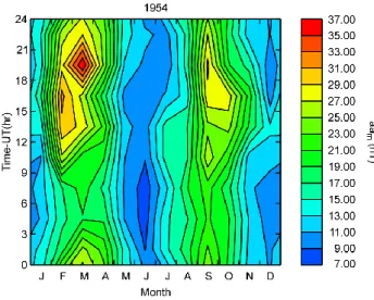
A diurnal/seasonal plot of the aam index for 1954 is given
in Fig. 7. For this year, the coefficient of the second har-monic for the aamindex is larger than was the case for 1996
(3.81 vs. 2.73; see Fig. 1). Normalizing the 1954 aamdata
for the ψ angle to obtain aam0removes ∼25% of the ampli-tude of the six-month wave (0.92/3.81). Because solar wind data are unavailable for 1954, we were unable to apportion the six-month wave in aam0between the Russell-McPherron and axial wind speed effects. There is no compelling evi-dence to suggest that one or the other is dominant, however. Correlating the 8×12 diurnal/seasonal variation plot of aam0 for 1954 with the Russell-McPherron and BO angles yields r = −0.49 and r = 0.59, respectively (statistically identi-cal).
Using Eq. (1), we reproduced the amplitude of the six-month wave in aam0values observed for 1954 by artificially
E. W. Cliver et al.: Origins of the semiannual variation 97
Fig. 6. Schematic showing how high-speed streams from polar
coronal holes can contribute to the semiannual variation of geomag-netic activity via an axial effect (after Bohlin, 1977).
increasing the amplitude of the six-month wave in either v or
Bs data from 1996 (by increasing monthly averages of these
parameters by a fixed percentage (5% for v, 10% for Bs)
dur-ing the six equinoctial months and decreasdur-ing them by the same percentage during solstitial months) and using monthly observed values from 1996 for the other parameter. Since the enhanced amplitudes of the semiannual variations in v or Bs
that were required to model the semiannual variation in aam0 were within the ranges of variability of these parameters for recent solar cycle decline/minimum epochs, there is no rea-son to suspect that the mechanisms giving rise to the strong six-month wave in aam0in 1954 were qualitatively different from those (i.e. the axial wind speed and Russell-McPherron effects) acting in 1996.
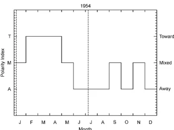
Svalgaard (1972) introduced a polarity index of the inter-planetary magnetic field based on diurnal patterns observed in ground-based polar magnetograms. Basically, a day is classified as having toward (away) polarity if the vertical component of the magnetic field at a near pole station has a broad, positive (negative) perturbation between magnetic noon and local noon. A third “mixed” classification is used for days that do not fit neatly into either the toward or away groups. If we count mixed polarity days as half favourable and half unfavourable, we find that, similarly to 1996, 62% of all days during 1954 had a favourable Russell-McPherron polarity (Fig. 8). Power spectral analysis of the aamdata in
Fig. 1a yields a strong peak at 27 days, indicating persistent recurrent storms (see Tandon, 1956), and solar eclipse obser-vations at mid-1954 (Fig. 9, taken from Vsekhsvjatsky, 1963; see also Schatten et al., 1978) reveal a streamer belt (base of the HCS) aligned with the solar equator.
2.4 The semiannual variation of geomagnetic activity in 1954 and 1996 and the 22-year variation of geomag-netic activity
The “halfwave rectifier” nature of the magnetosphere (Arnoldy, 1971; Burton et al., 1975) implies that
geomag-Fig. 7. Diurnal/seasonal variation of the aamindex during 1954.
netic activity will be enhanced via the Russell-McPherron effect when the Rosenberg-Coleman polarity effect produces enhanced positive polarity in spring and negative polarity in fall. Due to solar polarity reversal every 11 years at solar maximum, such conditions occur at alternate solar minima, contributing to an observed 22-year variation in geomagnetic activity (Chernosky, 1966; Cliver et al., 1996). This explana-tion for the 22-year geomagnetic cycle was first pointed out by Russell and McPherron (1973). The years 1954 and 1996 are separated by ∼2 × 22 years and are thus a manifestation of this periodicity.
3 Summary and discussion
We have examined the cause of the semiannual variation of geomagnetic activity for two solar minimum years in which the six-month wave is apparent in daily averages of the aam
index. During these years, both the Russell-McPherron and axial mechanisms make much larger contributions (each ac-counting for ∼33% of the total) to the semiannual variation than usual. For comparison, Cliver et al. (2000) and Sval-gaard et al. (2002) found that, in general, these two mech-anisms combined contribute only ∼30% to the six-month wave, with the remainder due to the equinoctial effect. 3.1 What was different about 1954 and 1996?
Years such as 1954 and 1996 with strong, well-defined semi-annual variations are rare, with only these two years out of 131 meeting our selection criteria (Sect. 2.1). What was un-usual about these years? As seen in Figs. 4 and 8 the solar wind polarity, rather than being more or less evenly mixed throughout the year, as it is in long-term averages, was pref-erentially inward in spring and outward in fall, circumstances that favour the creation of a southward field in the GSM co-ordinate system under the Russell-McPherron effect. The preference for one solar magnetic field polarity during the first half of the year and the other during the second half is
98 E. W. Cliver et al.: Origins of the semiannual variation
Fig. 8. Monthly solar wind magnetic polarity indices (Svalgaard,
1972) for 1954. A polarity was judged to be dominant during a month if it occurred for > 50% of the days. The dashed vertical lines indicate minima for the Russell-McPherron effect. Toward and away is with reference to the Sun.
an axial polarity effect discovered by Rosenberg and Cole-man (1969). It occurs during solar minimum years such as 1954 and 1996, when the heliographic equator and streamer belt are closely aligned (Figs. 5 and 9). At these times, the Earth will tend to sample one solar wind polarity when its heliographic latitude is positive and the opposite polarity for negative latitudes. Because the Sun reverses polarity every 11 years, the favourable polarities for the Russell-McPherron effect (inward in spring and outward in fall) occur at alter-nate solar minima. Thus, the combination of the Rosenberg-Coleman and Russell-McPherron effects contribute to the observed 22-year cycle of geomagnetic activity (Chernosky, 1966; Russell and McPherron, 1973; Cliver et al., 1996), and the strong semiannual variation in 1954 and 1996, separated by ∼2×22 years, is a reflection of the 22-year solar magnetic cycle.
The semiannual variation of geomagnetic activity in 1996 also benefited from a stronger than usual solar wind speed variation. The value of ∼18km s−1 we find for the coef-ficient of the second harmonic of the solar wind speed for 1996 (Fig. 3b) compares with ∼3km s−1for the 1963–1997 interval. A comparably enhanced (to 1996) six-month wave in solar wind speed is inferred for 1954. We attribute the semiannual variation in solar wind speed during 1954 and 1996 primarily to an axial effect involving the Sun’s polar coronal holes (Bohlin, 1977). The quasi-alignment of the he-liomagnetic and heliographic equators at solar minimum en-ables the Earth to access high-speed streams from alternate polar coronal holes on its excursions to ∼7◦N (S) heliolati-tude in September (March) (Fig. 6).
Four other solar minimum years (McKinnon, 1987) with favourable Rosenberg-Coleman polarity occurred during the 1868–1998 interval for which we have aamdata: 1889, 1913,
1933, and 1976. None of these years satisfied our selection
Fig. 9. Observation of the solar eclipse of 30 June 1954
(Vsekhsv-jatsky, 1963) showing the alignment of streamers with the solar equator.
criteria based on correlations of the aam data with the key
angles in the axial, Russell-McPherron and axial hypotheses. Correlation coefficients obtained were as follows:
1889 (r = 0.44(ψ ); r = −0.25(RM); r = −0.02(BO));
1913 (r = 0.48(ψ ); r = −0.43(RM); r = 0.23(BO));
1933 (r = 0.52(ψ ); r = −0.52(RM); r = 0.16(BO));
1976 (r = 0.59(ψ ); r = −0.35(RM); r = 0.37(BO)).
We note that the correlation coefficients for the Russell-McPherron mechanism for these four years are high in com-parison with all individual years from 1868–1998, ranking 63rd, 9th, 2nd, and 23rd, respectively. Differences in the degree of correlation with the three angles between the six favourable polarity minima are attributed to the vagaries of solar activity that can disrupt (or enhance) the seasonal-UT patterns of the geometry-based drivers of the semiannual variation.
3.2 The Rosenberg-Coleman effect
When considering the axial effect, one generally thinks of sunspot fields/magnetic field strength (Cortie, 1912) or coronal holes/solar wind speed (Bohlin, 1977) but not the Rosenberg-Coleman polarity effect. As first noted by Rus-sell and McPherron (1973), however, this semiannual varia-tion can play an important role at alternate solar minima.
A comparison of the six favourable (1889, 1913, 1933, 1954, 1976, and 1996) and six unfavourable (1878, 1901, 1923, 1944, 1964, and 1986) minimum years in the aamdata
set highlights the interplay of the Rosenberg-Coleman effect and the Russell-McPherron mechanism. For the average of the favourable years, correlation coefficients for the three hy-potheses are as follows: r = 0.76(ψ ); r = −0.56(RM); r = 0.48(BO). Corresponding coefficients for the unfavourable
years are: r = 0.60(ψ ); r = −0.16(RM); r = 0.44(BO).
The clear difference in the correlations with the RM angle contrasts with the relatively small differences for ψ and BO,
for which the responsible mechanisms are unaffected by the Sun’s polarity reversal.
E. W. Cliver et al.: Origins of the semiannual variation 99 3.3 Excitation/modulation and external vs. internal sources
of the semiannual variation
Mayaud (1974a) distinguished between excitation and mod-ulation mechanisms for the semiannual variation. Excita-tion mechanisms include the axial and Russell-McPherron effects which increase solar wind speed and southward field strength, respectively, at the equinoxes. In comparison, the equinoctial mechanism is thought to modulate the response of the magnetosphere to the solar wind input by reducing energy transfer at the solstices (Crooker and Siscoe, 1986). Cliver et al. (2000) used a “mountain building” vs. “valley digging” metaphor to illustrate the difference between exci-tation and modulation mechanisms.
Recently, Lyatsky et al. (2001) have suggested that nei-ther the amount of energy incident on the magnetosphere as in the axial and Russell-McPherron effects, nor the amount transferred to the magnetosphere via the equinoctial effect, is primarily responsible for the semiannual variation. Rather, they argued that the internal response of the system, based on the conductivity of the ionosphere in the polar regions, is the key factor. Because the variation of ionospheric conductiv-ity at any point on the Earth is governed by the solar zenith angle, the equinoctial hypothesis is the only one of the three classic hypotheses that could produce a conductivity pattern compatible with the pattern of geomagnetic activity apparent in Fig. 2. Lyatsky et al. (2001) showed that a diurnal/seasonal plot of the solar zenith angle for the midnight auroral oval of the more sunlit hemisphere had similar contours to that of the
ψangle and the am index.
One argument in favour of the coupling efficiency equinoctial hypothesis (vs. an equinoctial-based conductiv-ity variation) is the fact that the peak and minimum phases of average geomagnetic activity are shifted ∼5 days later than their theoretically predicted values (e.g˙peak average aa oc-curs on 27 March and 27 September (±2 day uncertainty) rather than on 21 March and 23 September) (Cliver et al., 2002). This delay has been interpreted by Mayaud (1974b) as an aberration effect due to the Earth’s orbital motion. If the seasonal variation was driven primarily by a conductiv-ity effect, one would expect the peak phase to occur at the “unaberrated” equinox.
3.4 Maximum size of the equinoctial effect
For both 1954 and 1996, the ψ -angle normalization removed
∼1 nT from the coefficient of the second harmonic in an FFT analysis of monthly values of aam. In fact, applying
this normalization to a perfectly flat diurnal/seasonal pattern for this index (with an amplitude of 19.3 nT corresponding to the average value of aam from 1868–1998) results in a
coefficient of ∼1 nT (vs. 1.26 nT for the actual aam matrix
for this interval). Thus, any value for the second harmonic coefficient of aam greater than ∼1 nT (for an annual
aver-age ∼19 nT), as observed for 1954 (3.8 nT; annual averaver-age = 17.2 nT) and 1996 (2.7 nT; annual average = 18.5 nT), indi-cates contributions from other factors, such as the axial and
Russell-McPherron mechanisms or randomness in solar ac-tivity. Over the long run of data, from 1868-present, these other factors are only of secondary importance, as evidenced by the close fit of the diurnal/seasonal pattern of geomag-netic activity to that predicted by the equinoctial hypothe-sis (McIntosh, 1959; Svalgaard, 1977; Cliver et al., 2000) and various calculations (e.g. Berthelier, 1976; Cliver et al., 2000; Svalgaard et al., 2002), indicating the dominance of the equinoctial effect.
Acknowledgements. We thank Nick Arge for help with the identifi-cation of the sources of high-speed streams in 1996 and the referee for helpful comments. This work was supported by AFRL Contract No. F19628-00-C-0089.
Topical Editor T. Pulkkinen thanks P. O’Brien for his help in evaluating this paper.
References
Arge, C. N., Odstrcil, D., Pizzo, V. J., and Mayer, L. R.: Improved method for specifying solar wind speed near the Sun, Proc. 10th Solar Wind Conference (submitted), 2002.
Arnoldy, R. L.: Signature in the interplanetary medium for sub-storms, J. Geophys. Res., 76, 5189, 1971.
Bame, S. J., Goldstein, B. E., Gosling, J. T., Harvey, J. W., McCo-mas, D. J., Neugebauer, M., and Phillips, J. L.: Ulysses observa-tions of a recurrent high speed solar wind stream and the helio-magnetic streamer belt: Geophys. Res. Lett., 20, 2323, 1993. Bartels, J.: Eine universelle Tagsperiode der erdmagnetischen
Ak-tivit¨at, Meteorol. Z., 42, 147, 1925.
Bartels, J.: Terrestrial-magnetic activity and its relation to solar phe-nomena, Terr. Mag. Atmos. Electr., 37, 1, 1932.
Berthelier, A.: Influence of the polarity of the interplanetary mag-netic field on the annual and diurnal variation of geomagmag-netic activity, J. Geophys. Res., 81, 4546, 1976.
Bohlin, J. D.: Extreme-ultraviolet observations of coronal holes, Solar Phys., 51, 377, 1977.
Burton, R. K., McPherron, R. L., and Russell, C. T.: An empirical relationship between interplanetary conditions and Dst, J. Geo-phys. Res., 80, 4204, 1975.
Chernosky, E. J.: Double sunspot-cycle variation in terrestrial-magnetic activity, J. Geophys. Res., 71, 965, 1966.
Cliver, E. W., Boriakoff, V., and Bounar, K. H.: The 22-year cycle of geomagnetic and solar wind activity, J. Geophys. Res., 101, 27 091, 1996.
Cliver, E. W., Kamide, Y., and Ling, A. G.: Mountains versus val-leys: The semiannual variation of geomagnetic activity, J. Geo-phys. Res., 105, 2413, 2000.
Cliver, E. W., Kamide, Y., Ling, A. G., and Yokoyama, N.: Semi-annual variation of the geomagnetic Dst index: Evidence for a dominant nonstorm component, J. Geophys. Res., 106, 21 297, 2001.
Cliver, E. W., Kamide, Y., and Ling, A. G.: The semiannual vari-ation of geomagnetic activity: Phases and profiles for 130 years of aa data, J. Atmos. Sol. Terr. Phys., 64, 47, 2002.
Cortie, A. L.: Sunspots and terrestrial magnetic phenomena, 1898– 1911: The cause of the annual variation in magnetic distur-bances, Mon. Not. Roy. Astron. Soc., 73, 52, 1912.
Crooker, N. U. and Siscoe, G. L.: On the limits of energy transfer through dayside merging, J. Geophys. Res., 91, 13 393, 1986.
100 E. W. Cliver et al.: Origins of the semiannual variation
Feynman, J. and Crooker, N. U.: The solar wind at the turn of the century, Nature, 275, 626, 1978.
Galvin, A. B. and Kohl, J. L.: Whole Sun Month at solar minimum: An introduction, J. Geophys. Res., 104, 9673, 1999.
Hoeksema, J. T.: Extending the sun’s magnetic field through the three dimensional heliosphere, Adv. Space Res., 9(4), 141, 1989. Hundhausen, A. J.: An interplanetary view of coronal holes, in: Coronal Holes and High Speed Wind Streams, edited by Zirker, J. B., Colorado Associated University Press: Boulder, CO, p. 225, 1977.
Lyatsky, W., Newell, P. T., and Hamza, A.: Solar illumination as the cause of the equinoctial preference for geomagnetic activity, Geophys. Res. Lett., 28, 2353, 2001.
Mayaud, P. N.: The aa indices: A 100 year series characterizing the magnetic activity, J. Geophys. Res., 77, 6870, 1972.
Mayaud, P. N.: Comment on “Semiannual variation of geomagnetic activity” by C. T. Russell and R. L. McPherron, J. Geophys. Res., 79, 1131, 1974a.
Mayaud, P. N.: Variation semi-annuelle de l’activit´e magn´etique et vitesse du vent solaire, Comptes Rendus Academie des Sciences, Paris, 278, 139, 1974b.
Mayaud, P. N.: Derivation, Meaning, and Use of Geomagnetic In-dices, American Geophysical Union: Washington, DC, 1980. McIntosh, D. H.: On the annual variation of magnetic disturbance,
Phil. Trans. Roy. Soc. London, Ser. A., 251, 525, 1959. McKinnon, J. A.: Sunspot Numbers: 1610–1985, Report UAG-95,
World Data Center A: Boulder, CO, 1987.
O’Brien, T. P. and McPherron, R. L.: Seasonal and diurnal variation of Dst dynamics, J. Geophys. Res., 107, 1341, doi:10.1029/2002JA009435, 2002.
Phillips, J. L., Bame, S. J., Feldman, W. C., Goldstein, B. E., Gosling, J. T., Hammond, C. M., McComas, D. J., Neugebauer, M., Scime, E. E., and Suess, S. T.: Ulysses solar wind plasma observations at higher southerly latitudes, Science, 268, 1030, 1995.
Rosenberg, R. L. and Coleman, P. J.: Heliographic latitude
depen-dence of the dominant polarity of the interplanetary magnetic field, J. Geophys. Res., 74, 5611, 1969.
Russell, C. T. and McPherron, R. L.: Semiannual variation of geo-magnetic activity, J. Geophys. Res., 78, 92, 1973.
Russell, C. T. and McPherron, R. L.: Reply, J. Geophys. Res., 79, 1132, 1974.
Sabine, E.: On periodical laws discoverable in the mean effects of the larger magnetic disturbances – No. III, Phil. Trans. Roy. Soc. London, 146, 357, 1856.
Smith, E. J. and Thomas, B. T.: Latitudinal extent of the helio-spheric current sheet and modulation of galactic cosmic rays, J. Geophys. Res., 91, 2933, 1986.
Schatten, K. H., Scherrer, P. H., Svalgaard, L., and Wilcox, J. M.: Using dynamo theory to predict the sunspot number during cycle 21, Geophys. Res. Lett., 5, 411, 1978.
Svalgaard, L.: Interplanetary magnetic-sector structure, 1926– 1971, J. Geophys. Res., 77, 4027, 1972.
Svalgaard, L.: Geomagnetic activity: Dependence on solar wind parameters, in: Coronal Holes and High Speed Wind Streams, edited by Zirker, J. B., Colorado Associated University Press: Boulder, CO, 371, 1977.
Svalgaard, L., Cliver, E. W., and Ling, A. G.: The semiannual vari-ation of great geomagnetic storms, Geophys. Res. Lett., 29, doi: 029/2001GL014145, 2002.
Tandon, J. N.: Geomagnetic activity and solar M-regions for the current epoch of the sunspot minimum, Indian J. Phys, 30, 153, 1956.
Temerin, M. and Li, X.: A new model for the prediction of Dst on the basis of the solar wind, J. Geophys. Res., 107, 1472, 2002. Vsekhsvjatsky, S. K.: The Structure of the Solar Corona and the
corpuscular streams, in: The Solar Corona, Proc. Int. Astr. Union Symp. 16, edited by Evans, J. W., Academic Pub: New York, p. 271, 1963.
Zhao, X. P., Hoeksema, J. T., and Scherrer, P. H.: Changes of the boot-shaped coronal hole boundary during Whole Sun Month during sunspot minimum, J. Geophys. Res., 104, 9735, 1999.