Intermittent Rivers and Biodiversity. Large scale analyses between hydrology and ecology in intermittent rivers

(1)

HAL Id: hal-02600343

https://hal.inrae.fr/hal-02600343

Submitted on 16 May 2020

HAL is a multi-disciplinary open access archive for the deposit and dissemination of sci-entific research documents, whether they are pub-lished or not. The documents may come from teaching and research institutions in France or abroad, or from public or private research centers.

L’archive ouverte pluridisciplinaire HAL, est destinée au dépôt et à la diffusion de documents scientifiques de niveau recherche, publiés ou non, émanant des établissements d’enseignement et de recherche français ou étrangers, des laboratoires publics ou privés.

rivers

Q. Blanchard

To cite this version:

Q. Blanchard. Intermittent Rivers and Biodiversity. Large scale analyses between hydrology and ecology in intermittent rivers. Environmental Sciences. 2014. �hal-02600343�

(2)

Intermittent Rivers and Biodiversity

Large scale analyses between hydrology and

ecology in intermittent rivers.

Report for the courses of specialization in the Management of

Natural Habitats (GMN) for the obtaining of a Master in

engineering in ENGEES

(3)

Quitterie Blanchard Final dissertation for an engineer degree 2014

(4)

Quitterie Blanchard Final dissertation for an engineer degree 2014 ENGEES

AGROPARISTECH

Blanchard Quitterie August 2014 IRSTEA

Intermittent Rivers and Biodiversity

Large scale analyses between hydrology and ecology in intermittent rivers.

Courses of specialization in the Management of

Natural Habitats (GMN)

(5)

(6)

(7)

Quitterie Blanchard Final dissertation for an engineer degree 2014 Abstract

Intermittent rivers are characterized by a temporary interruption of their flow which can manifest in a variety of ways, as much on a spatial scale as on a temporal one. This particular aspect of intermittent river hydrology gives rise to unique ecosystems, combining both aquatic and terrestrial habitats. Neglected for a long time by scientists and once considered biologically depauperate and ecologically unimportant, these fragile habitats are nowadays acknowledged for their rendered services. Furthermore, the dynamics of these ecosystems which have been recently revealed, speak in favor of a unique and fragile biodiversity. This project aims to provide a better understanding of the ecological responses linked to this intermittency phenomenon. To reach this aim, hydrological and biological data from rivers in France and Australia, supplied thanks to the collaboration of scientists within IRBAS (Intermittent Rivers Biodiversity Analyses and Syntheses) will be linked and analyzed in this work. This study will consist of a comparative statistical analysis of intermittent versus perennial rivers, following a preliminary matching of the biological and hydrological data using GIS tools. This preliminary analysis revealed that only the Australian data could be analyzed. Strong differences were not found between intermittent and perennial rivers in terms of their biodiversity, but they had significantly different flow regimes and physico-chemical characteristics, intermittent rivers tending to have greater flow variability but lower dissolved oxygen levels. The absence of confirmation of a difference in richness between intermittent and perennial rivers may indicate the Australian biota have high resilience to intermittence, at least for the sites that have been studied. However, if climate and human use of water continues to change, the biota may in the future experience novel conditions, such as unprecedently long dry periods, that could jeopardize their resilience. The ongoing study of intermittent rivers will no doubt continue to expand the ecological understanding of these systems and improve their management and protection.

“Résumé”

Les rivières intermittentes sont caractérisées par une interruption temporaire de leurs cours pouvant se manifester de façons très variées, tant à l’échelle spatiale que temporelle. Ce fonctionnement particulier et très variable, donne lieu à la formation d’écosystèmes uniques, mêlant à la fois habitats aquatiques et terrestres. Bien longtemps négligés des scientifiques, les jugeant écologiquement pauvres et sans intérêt écologique, ces milieux fragiles sont aujourd’hui d’un intérêt reconnu. De plus, les dynamiques de ces écosystèmes qui ont récemment été dévoilées, plaident en faveur d’une biodiversité unique et fragile. Ce projet a pour objectif une meilleure compréhension des réponses écologiques associées à ce phénomène d’intermittence. Pour cela, des données hydrologiques et biologiques fournies grâce à la collaboration de chercheurs, dans le cadre du projet IRBAS (Analyse et Synthèse de la Biodiversité des Rivières Intermittentes) seront analysées au travers de ce projet. Cette étude consistera en une analyse statistique comparative de rivières intermittentes et pérennes, après un travail préliminaire d’appariement des données biologiques et écologiques, grâce à l’emploi d’un SIG. Cette analyse préliminaire a permis de déterminer que seules les données australiennes pouvaient être étudiées. Si de fortes différences n’ont pu être mises en évidence entre les rivières intermittentes et pérennes, en termes de biodiversité, les stations présentaient cependant des régimes, et des paramètres physico-chimiques très distincts, les cours d’eau intermittents marqués par une forte variabilité de courant ou encore un faible taux d’oxygène dissous. L’absence de confirmation d’une différence de richesse entre les rivières intermittentes et pérennes, pourraient témoigner d’une haute résilience face à l’intermittent, du moins pour les sites étudiés. Cependant, si le climat et les pressions anthropiques continuent à changer, les écosystèmes pourraient devoir faire face à des conditions inédites, comme des asséchements d’une durée sans précédents, qui pourraient menacer cette résilience. Les études à venir dédiées aux rivières intermittentes vont sans doute continuer à accroître la

(8)

1

Acknowledgments

I would like to express the deepest appreciation to my supervisor Dr Catherine LEIGH for her continuous support, her patience, motivation, enthusiasm and immense knowledge. Her guidance helped me in all the time of research and writing of this work. I could not have imagined having a better advisor and mentor. My sincere thanks to Mr Thibault DATRY who offered me the internship, and who was always available whenever I needed him, even from Bolivia!

My gratitude also goes to my advisor Mr Christian PIEDALLU. His good advice, support and friendship have been invaluable on both an academic and a personal level. It was such a relief to be able to get his support anytime I felt like it.

A very special thanks to the DYNAM team, inside the MALY Unit at IRSTEA LYON for their help, friendship and support. Among them are:

Jasper HOEVE and Stephan DEVRIES, Dutch students, who were part of the IRBAS project and without whom this work would not have been achieved;

Mr Nicolas LAMOUROUX who first shared his office, then his knowledge with me;

and last but not the least Mr Hervé PELLA, for his skills in ARCGIS which were a big help for me, ignorant as I was at the beginning.

Finally I would like to thank my boyfriend Florent BUTRUILLE, my grand-mother and especially my mother, as well as all my friends and particularly Anaïs KARCH and Emilie CAPORUSSO for their continuous help, patience and support.

(9)

2

Cautionary note

This research project is aligned with the IRBAS project: Intermittent River Biodiversity Analysis and Synthesis (http://www.irbas.fr/) supported by IRSTEA and by CESAB (Center for Synthesis and Analysis of Biodiversity), which is funded jointly by FRB (French Foundation for Research & Biodiversity) and ONEMA (French National Agency for Water & Aquatic Environments).

(10)

3

Acknowledgments ... 1

Cautionary note ... 2

Table of contents ... 3

Tables and figures ... 5

Table of ANNEXE ... 7

Table of acronyms ... 8

Introduction... 9

Part One: definition of the subject ... 11

I. Intermittent Rivers ... 11

1. Definition ... 11

2. Importance ... 12

II. The international context ... 12

1. Climate change and consequences of these changes on the IR ... 12

2. The IRBAS project : Intermittent Rivers Biodiversity Analyses and Synthesis ... 13

Part Two: Preliminary work ... 14

I. First aims of the preliminary work: collecting biological and hydrological data to combine information ... 14

II. Collecting the data ... 15

1. Biological samples, for France and Australia ... 15

2. Hydrological data ... 16

III. Geolocalisation ... 17

1. The principle ... 17

2. Two different methods to reach the same goal ... 19

1. The “manual method” ... 19

2. The “systematic” method ... 19

Part Three: Matching the sites to link biological and hydrological data ... 22

I. Main principle ... 22

1. Context and goal to reach ... 22

2. Usable parameters : need to get information from datasets ... 22

(11)

4

II. Concrete methods and tools used ... 25

1. ARCGIS and the distance study ... 25

1. Buffer zone ... 25

2. Method to assess the length of the flow path between two stations ... 26

2. France ... 28

1. Qualitative selection applicable for the French dataset ... 28

2. Other solutions examined: getting round the lack of stations ... 30

3. Limits of the French dataset ... 32

3. Australia ... 33

1. Presentation of the dataset ... 33

2. Choices to make for the Australian selection ... 36

3. “Risk” couples for intermittent dataset: ... 37

III. Data final management: creating pairs of Australian couples ... 42

1. The selection method ... 42

2. Testing the usability of the data selected ... 45

3. The creation of another set of data with an optimization of the repartition ... 47

Part Four: Analyzing the pairs ... 49

I. Data management ... 49

1. The available metrics, presentation of the data ... 49

1. Biological data: Abundances for macro-invertebrates ... 49

2. Environmental and flow metrics... 49

2. Primer and the calculation of the diversity metrics ... 52

3. Correlations and redundancies: Pearson’s and Spearman’s correlation test ... 52

1. Adjustments required: to reach a Gaussian repartition ... 52

2. Checking and correcting the factors to follow a Normal distribution. ... 53

3. The correlation calculations ... 53

4. The final list of metrics saved ... 57

II. First tests: Showing differences between intermittent and perennial couples ... 58

1. The paired and the unpaired tests ... 58

2. The results of the tests applied to the two datasets ... 60

Part Five: Discussion and conclusions about the analyses ... 63

I. The meaning of the results ... 63

1. Paired analysis ... 64

2. The unpaired analysis ... 64

II. Conclusions, discussions and options ... 65

Conclusion ... 66

References ... 68

(12)

5

Tables and figures

Table 1: Geographic and geologic classes of temporary rivers, and mechanisms controlling water loss, extracted and modified from Larned et al. 2010. ____________________________________________ 11 Table 2: Information about data availability and classification of hydrological gaging stations, extracted and modified from (Hoeve & De Vries 2014). ______________________________________________ 16 Table 3: Number of stations and nature of samples from the initial dataset (NA=Not applicable) _____ 23 Table 4: Number and nature of available bio-monitoring _____________________________________ 23 Table 5: Number and nature of selected stations ____________________________________________ 23 Table 6: Final number of stations used ___________________________________________________ 24 Table 7: Possible coupling results for France between 303 biological stations and 1008 hydrological stations including 66 intermittent ones. ___________________________________________________ 26 Table 8: Linear distances among biological and hydrological stations in France and in Australia ____ 27 Table 9: Summary of the results for the process of matching the sites ___________________________ 29 Table 10: Information about potential couples for France ____________________________________ 30 Table 11 Nature of flow regime of Australian hydrological stations _____________________________ 33 Table 12: Summary of the possible links to make between the stations ___________________________ 33 Table 13 Information about the number of usable intermittent couples __________________________ 34 Table 14 Information about the number of usable perennial couples ____________________________ 34 Table 15: Spatial repartition of the stations _______________________________________________ 35 Table 16: Criteria to help the choice of the Australian couples ________________________________ 37 Table 17: Information about couples that needed further verification of suitability to include in analyses38 Table 18: Information about the potential couples to link with the hydrological station"NT-8150098" _ 39 Table 19: Information about the potential couples to link with the hydrological station"QLD-132001a" 40 Table 20: Information about the potential couples to link with the hydrological station"QLD-134001b 41 Table 21: Description of the mark system _________________________________________________ 44 Table 22: Results of the statistic tests to check for the usability of the dataset of the 21 pairs ________ 46 Table 23: Definitions of the environmental metrics used(Australian and New Zealand Environment and Conservation Council 2000) ____________________________________________________________ 50 Table 24: Description of the flow metrics from Kennard’s work on the classification of regimes(Kennard et al. 2010) _________________________________________________________________________ 51 Table 25: Definition of the diversity metrics used ___________________________________________ 52 Table 26: Selected metrics and transformations ____________________________________________ 53 Table 27: Pearson's correlations ________________________________________________________ 54 Table 28: Spearman's correlations_______________________________________________________ 54 Table 29: Metrics used for the analyses ___________________________________________________ 57 Table 30: Results of the statistic tests and link influence ______________________________________ 60 Table 31: Summary of the results for the statistical tests of difference between intermittent and perennial sites _______________________________________________________________________________ 63

(13)

6

Figure 1: Methodology for the preliminary phase ___________________________________________ 14 Figure 2: The SANDRE, the ONEMA and AUSRivAS emblems ________________________________ 15 Figure 3: Example of an Australian biological station where the automatic snapping function available in ARCGIS would not provide an appropriate solution. ________________________________________ 18 Figure 4: Criteria for sorting for the different datasets. ______________________________________ 21 Figure 5: Localization of couples between intermittent hydrological stations and biological stations from the RCR within 50km _________________________________________________________________ 28 Figure 6: Sub-captions showing the flow path relations between the intermittent hydrological station (blue star) and the most relevant biological station to be associated with (dots). _______________________ 31 Figure 7: Nature of flow regime of Australian and French hydrological stations __________________ 33 Figure 8: Repartition of the intermittent and perennial sites. __________________________________ 36 Figure 9: ARCGIS caption of couple n°2 __________________________________________________ 39 Figure 10: ARCGIS caption of couple n°8 _________________________________________________ 40 Figure 11: ARCGIS caption of the Couple n°9 _____________________________________________ 41 Figure 12: Summary of the second step of linking the couples after the preliminary phases __________ 42 Figure 13: The 28 intermittent sites involving a hydrological and a biological station with the ID of the biological station, selected for the study. __________________________________________________ 43 Figure 14: Description of the methodology to build analyzable datasets. ________________________ 44 Figure 15: Explanations about the program written in R _____________________________________ 48 Figure 16: Correlations between diversity metrics __________________________________________ 55 Figure 17: Correlations for the flow metrics with the Pearson's method _________________________ 55 Figure 18: Correlations for the flow metrics with Spearman's coefficient ________________________ 56 Figure 19: Characteristics of the unpaired data set of 28 intermittent sites and 28 perennial sites ____ 58 Figure 20: Characteristics of the paired data set of 21 intermittent sites and 21 perennial sites ______ 59 Figure 21: Comparisons between the geographical repartition of the sites among the unpaired dataset 59 Figure 22: Simplified map of the Australian various climates. Source : www.australia.edu __________ 62

(14)

7

Table of ANNEXE

ANNEXE 1 : 48 intermittent couples of hydrological and biological station ______________________ 72 ANNEXE 2:48 intermittent couples of hydrological and biological station with calculations and tools for the selection ________________________________________________________________________ 74 ANNEXE 3: Australian risk couples _____________________________________________________ 76 ANNEXE 4: 28 intermittent couples kept for the investigations ________________________________ 80 ANNEXE 5: 21 pairs of intermittent and perennial couples associated depending on their localization 81 ANNEXE 6: Program in R for the optimization of the repartition ______________________________ 82 ANNEXE 7 : List of taxa ______________________________________________________________ 84 ANNEXE 8 List of taxa specific to intermittent and perennial sites _____________________________ 85 ANNEXE 9: Log adjustment used to reach a Normal distribution, example of the turbidity for the unpaired dataset ____________________________________________________________________________ 86 ANNEXE 10: Correlation tables for the environmental metrics ________________________________ 87 ANNEXE 11: Correlation tables for the flow metrics ________________________________________ 88 ANNEXE 12: Correlation tables for the flow metrics ________________________________________ 89 ANNEXE 13: Results and p-values of the statistic tests among the paired and unpaired couples _____ 91 ANNEXE 14: Climate classification of Australia(Bureau of Meteorology) _______________________ 94

(15)

8

Table of acronyms

ANU : Australian National University

ANUDEM : Australian National University Digital Elevation Model

ARCGIS : Aeronautical Reconnaissance Coverage Geographic Information System BD CARTHAGE® : Base de Données Carthage (Carthage Data Base)

BD ALTI : Base de Données Altimétriques (Altitude data base)

CESAB : Centre de Synthèses et d’Analyses de la Biodiversité (Center of Syntheses and analyses of the Biodiversity)

DEM : Digital Elevation Model

DYNAM : Laboratoire Dynamiques, Modèles en écohydrologie ESRI :Environmental Systems Research Institute

GIS : Geographic Information System

GMN : Gestion des Milieux Naturels (Management of Natural Habitats) I : Intermittent

ID : Identity

IGN : Institut Géographique National (Geographic National Institute) IPCC :The Intergovernmental Panel on Climate Change

IR : Intermittent River

IRBAS : Intermittent rivers and Biodiversity Analyses and Synthesis NA : Not Applicable

NSW: New South Wales

ONEMA : Office National de l’Eau et des Milieux Aquatiques (National Office for Water and Aquatic Habitats)

P : Perennial

PPMC : Pearson Product-Moment Correlation QLD : Queensland

RCR : Réseau de Contrôle et de Référence (Reference Network of Control) RCS : Réseau de contrôle et de surveillance (Control and Surveilliance Network) RHT : Réseau Hydrographique Théorique (Theoretical Hydrological Network) SA : South Australia

SANDRE : Service d’Administration des Données et Référentiels sur l’Eau (National Data Reference Center for Water)

TAS : Tasmania VIC : Victoria

(16)

9

Introduction

In a century of increasing human demands in resources, the achievement of a sustainable management of water is one of the key issues. The acknowledgement of a need to protect ecosystems is now recognized by a majority of governments, and is becoming increasingly incorporated into land and water management guidelines and policy. A huge number of ecosystems are water-dependent, many of which are highly biodiverse, provide multiple ecosystem services, and are of high conservation value. This increasing anthropic pressure is therefore threatening water-dependent habitats, and this phenomenon is exacerbated in the context of global warming, due to its direct and indirect impacts on river flow regimes, ecosystem processes and organisms.

This is just one of the reasons why the terms hydroecology and ecohydrology are being used increasingly in the scientific literature, including from the perspective of sustainable water management. This reflects an increasing willingness to protect and respect ecosystems by governments, the public and the research community.

Despite this awareness, the protections, when they are established are often inappropriate or inadequate, due to the complexity of flow patterns, and need to be improved. A better understanding of these systems, particularly their hydroecology, is needed to better manage, conserve or restore these systems for the betterment of society, economy and the environment.

In addition, the world’s river systems encompass a wide diversity of flow regimes, but not all are understood equally. Intermittent rivers can be defined as rivers that periodically cease to flow, and are therefore distinct from perennial streams, which flow throughout the year and have traditionally been the focus of river research.

Intermittent rivers have been considered as ecologically poor, but a recent increase in research of these systems has allowed the acknowledgement that their very specific but diverse hydrological dynamics likely elicit diverse ecologic responses and support both aquatic and terrestrial communities.

However, the huge variability in patterns of flow intermittency requires more focus to be understood properly. This internship was based on the need to understand better the science of hydroecology, inside the specificity of intermittent rivers, namely by linking a biological response to intermittent rivers.

IRSTEA, the National Research Institute of Science and Technology for Environment and Agriculture, which hosts some of the members of the IRBAS project (Intermittent Rivers Biology Analysis and Synthesis), supports research in favor of the reasonable management of natural resources and habitats. Thanks to this collaboration among influential scientists from both IRBAS and IRSTEA, biological and hydrological data was collected and needed to be associated and studied.

(17)

10

Quitterie Blanchard Final dissertation for an engineer degree 2014 The first part of this work will be devoted to a more accurate definition of the global context of the research. In Part Two, the available data will be introduced. Then, after a data management process in Part Three, the concrete links between hydrology and ecology will be achieved to reach the analyses in Part Four . Finally, conclusions of the work will be drawn in the fifth and final part of this report.

(18)

11

Part One: definition of the subject

I. Intermittent Rivers

1. Definition

Intermittent rivers are defined as rivers that periodically cease to flow (Datry, Larned & Tockner 2014b). Thus, this simple definition gives birth to an extreme variability of hydrological and hydraulic behaviors that can occur in rivers of many different classes and all over the world, in most climates, and not only in dry regions (Table 1). The flow cessation can be caused by several factors such as seepages through a permeable bed, or runoff recession (Table 1).

The cessation of flow in intermittent rivers is usually associated with complete loss of surface water at some point(s) along the water course, but also with the creation of isolated pools of standing water (lentic habitat) in between sections or periods of dry channel or flowing waters. The intermittency regime thus creates a very special longitudinal and temporal dynamic consisting of the alternation of terrestrial and aquatic habitats, leading to a unique biodiversity.

In spite of the complexity of this subject, a certain quantity of scientific literature can be found that characterizes and explains these hydrological dynamics. However, even if intermittent rivers and streams have been described and studied in several countries, there is still a great lack of knowledge, especially since the number of temporary rivers is tending to increase, as well as the intensity of the intermittency (Larned et al. 2010).

Table 1: Geographic and geologic classes of temporary rivers, and mechanisms controlling water loss, extracted and modified from Larned et al. 2010.

Class Predominant mechanisms of water loss

Snowmelt and glacial meltwater Cessation of melting/ablation, freezing of surface and

shallow subsurface water

Perched and semi-perched alluvial Transmission loss, depletion of bank storage and floodplain aquifer

Non-perched, in arid and semi-arid regions

Depletion of surface water and shallow groundwater by direct evaporation and evapotranspiration

Zero-order and headwater streams Cessation of overland flow, depletion of saturated soil water or hill slope aquifer, macro pore recession

Permafrost Soil freezing, soil water and wetland recession

Karstic Transmission loss, cessation of spring discharge

Lake outlets Lake level drops below outlet elevation

(19)

12

Quitterie Blanchard Final dissertation for an engineer degree 2014 While Table 1 describes intermittency in terms of geographic and geologic classes, intermittent rivers can also be classified in terms of their hydrological (‘flow’) regime. The hydrological classification of rivers is one of the most important tasks in hydrological ecology. Indeed, the flow regime is an essential parameter to determine or explain the biodiversity of a habitat (Poff et al. 1997). Although there are many ways in which flow regimes can be classified, this step is considered essential in the perspective of considering the ecological relevance of a particular hydrological regime pattern.

2. Importance

Intermittent rivers also have a very important role in hydrological dynamics, and consequently, in social and economic issues. They are involved in some important ecological processes, especially fluxes, depending on their class (Table 1). They often play the role of a buffer, since they can mitigate the effect of a flood (Foody, Ghoneim & Arnell 2004), and in the same perspective, limit the consequences of a drought, transferring water to aquifers. In some countries, they are even the unique source of drinkable water and it is therefore easy to understand why they require accurate management, which can be achieved thanks to an understanding of their large scales patterns (Snelder et al. 2013).

Since the flow regime is one of the most important parameters that determine ecological response and behavior(Power et al. 1995; Poff et al. 1997; Richter et al. 2003), intermittent rivers can be considered ecologically significant ecosystems. Their dynamics include advanced and retreating flows, and this alternation of dry periods and floods creates some very special habitats and characteristics (Corti 2013; Datry et al. 2014a). Fluctuations in discharge can create particular responses, such as basins of upwelling groundwater, during an advancing front (Doering et al. 2007). Recessions periods may also induce chains of pools (Boulton 2003). These alternations of advance and retreat also provide a source of nutrient that is often greater than for perennial streams (Larned et al. 2010).

These very particular aspects mean that intermittent rivers require specific and in-depth ecological understanding to guarantee their appropriate management and protection.

II. The international context

1. Climate change and consequences of these changes on the IR

According to estimations, the proportion of intermittent rivers among the global network is usually considered to be of the range of 30%, but since this calculation does not include low order streams (i.e. headwaters), the true proportion is more likely greater than 50%. Besides, in the latest 50 years, a large number of perennial streams have turned to perennial, due to increased human pressure involving water abstraction or perturbation in flows (Datry et al. 2014b).

(20)

13

Quitterie Blanchard Final dissertation for an engineer degree 2014 However, the number of intermittent rivers and the intensity of unusual events are still tending to increase, and in spite of the acknowledgement of this situation, the attention accorded to this kind of stream is still insufficient(Acuna et al. 2014). Policies and management devoted to this topic are often restricted and inadequate (Snelder et al. 2013). A greater focus is usually accorded to perennial rivers, and the scarcity of information about intermittent rivers characteristics should be addressed to tackle this imbalance.

2. The IRBAS project : Intermittent Rivers Biodiversity Analyses and Synthesis

Thanks to this awareness of this concerning lack of knowledge, some of the most influential scientists and researchers of this subject decided to exchange their skills and tools in favor of the improved ecological understanding of intermittent streams.

The project, initiated by Dr Thibault Datry, a French researcher at IRSTEA, is sponsored by the CESAB (the Center of Synthesis and Analyses of Biodiversity), and the funds are provided by both the FRB (Foundation for Research and Biodiversity) and the ONEMA (The National office of Water and Aquatic Habitats). It started in June 2013, and will finish at the end of 2015. Its main members are Dr Catherine Leigh, formally of Griffith University, Brisbane, Australia but now at IRSTEA, Lyon, France; Prof. Klement Tockner, from the Leibniz-Institute of Freshwater Ecology and Inland Fisheries (IGB), Berlin, Germany; Dr Nuria Bonada, from University of Barcelona, Spain; Dr. Clifford Dahm, from the University of New Mexico, Arizona, United States or America; Dr. Eric Sauquet, from IRSTEA, Lyon, France; Dr Scott Larned, from The National Institute of Water and Atmospheric Research( NIWA), Christchurch, New-Zealand, and other affiliated members and trainees.

The objectives of IRBAS are divided into three axes of study, namely the links between hydrology and climate, to lead to global patterns of intermittency, ecological responses to intermittent flow and finally, the fragmentation of habitats and the connections between them.

At the launching of the project, some workshops were conducted and the data was put together to start the investigations. Some hydrological measurements and bio-monitoring data came out of this collaboration for France, Australia, Spain and United-States, and needed to be analyzed together to meet the project’s expectations; a better understanding about the links between hydrology and ecology in intermittent rivers.

(21)

14

Part Two: Preliminary work

I. First aims of the preliminary work: collecting biological and hydrological data to

combine information

The aim of the preliminary work will be the association (‘coupling’) of the biological and the hydrological data from sampling stations in France and Australia that were identified by the IRBAS group (noting that the data from Spain and the United States were not yet available at the time of this project). At the end of the second part, a reasonable number of couples, i.e. about 30 hydrological stations linked to 30 biological stations, will be selected, assuming that analyses would be robust enough with this amount of stations (Figure 1).

Figure 1: Methodology for the preliminary phase

*: The method applied for the selection of the data is described on Figure 4 •Datasets from

hydrological and biological stations’ + networks of flow path

Selection of the data*according to several criteria •Usable dataset of stations fitting criteria’ Geolocalisation

on the network •Matching the

stations to the river flow path network in ARCGIS’ Matching the stations First goal: linking biological and hydrological data

(22)

15

II. Collecting the data

1. Biological samples, for France and Australia

For both France and Australia, the biological data consisted of abundance data, i.e. the taxa found in the biological stations.

For France, the samples were provided by the SANDRE (Figure 2), which is a network linking different actors in charge of water issues. This organization, driven by the ONEMA (The French National Agency for Water and Aquatic Environments) provides the collection of the total existing data about water (Figure 2). The data consisted of abundances of fish, macrophytes, macro-invertebrates and diatoms, with a specification of the taxa. Each station had a location given as GPS coordinates, and allowing its geolocalisation in GIS. Some of the stations were included in a special network, the referenced network, also known as RCR (Referenced Network of Control), listing the stations which were supposed to be the least impacted by human pressure, such as pollution or water resource development. Only this network of stations was used in the analyses (Villeneuve et al. 2009).

For Australia, the abundances were only concerning macroinvertebrates and were produced by AUSRivAS (AUStralian River Assessment System), a system used to assess the ecological health of Australian rivers. It was created by the NRHP (the National River Health Program) because the government was becoming more and more concerned about the condition of its inland waters. AUSRivAS was also separating the “Reference” stations from the others, depending on their level of human pressure (Cooperative Research Centre for Freshwater Ecology (Australia) & Environment Australia).

Australia is politically divided into 7 states and territories, and for AusRivAs, each uses its own protocol guide of sampling. Some of the hurdles associated were to homogenize this data to make them comparable (1. Biological data: Abundances for macro-invertebrates).

(23)

16

Quitterie Blanchard Final dissertation for an engineer degree 2014 2. Hydrological data

For France and Australia, the initial hydrological dataset depended on the results of previous studies. For France, it was originally scheduled to use Ton H. Snelder’s work, on the regionalization of patterns of flow intermittence from gauging stations records (Snelder et al. 2013). However, two Masters’ students from The Netherlands in charge of updating the hydrological classification of both the French and Australian stations according to intermittence were hired at the beginning of this study. It was finally decided to be worth waiting for the results of their work to start analyses using a more recent database that would be standardized across both countries (Hoeve & De Vries 2014).

Jasper Hoeve and Stefan de Vries worked on the four countries that initially took part of the project. After a selection of the gauging stations according to their low (human-induced) modifications of their hydrological regime, the students refreshed the classifications made previously, to select the most confident intermittent stations, which resulted in the final set of stations used for this study.

To summarize this work of selection, the main restrictions applied to the original French and Australian data (respectively provided by the data base HYDRO, and by the Australian government) concerned the data length, the minimum period of 0-flow, and the proportion of missing data (Hoeve & De Vries 2014). A minimum duration of data collection was fixed at 30 years, and was required for the estimations of long term trends that would be part of the IRBAS project to simulate intermittency. This length is also advised by The Intergovernmental Panel on Climate Change (IPCC) ( IPCC WGIII Fifth Assessment Report - Mitigation of Climate Change 2014) and should “encompass a range of climatic variations” (IPCC, n.d.). Then, a maximum of 5% of missing data was set, and finally to classify a river segment as intermittent, the mean daily discharge was equal or less than 0, 001 m3/s (required by the limited ability of gauging stations to quantify very low-to-zero flow). After an agreement between hydrological experts from the IRBAS team, the “intermittent” status was given to the gauging stations recording at least 5 zero flow days per year, to reduce the risk of including some false positives.

These selections, especially for France, have significantly reduced the total amount of available stations (Table 2).

Table 2: Information about data availability and classification of hydrological gaging stations, extracted and modified from (Hoeve & De Vries 2014).

France Australia

Intermittent 64 274

Perennial 966 160

Rejected (did not meet the selection criteria)

(24)

17

III. Geolocalisation

1. The principle

At this stage, defined flow path networks were needed for France and Australia in order to match the hydrological and biological sites, after making the sites correspond to a point on a stream, and to reach the measurement of linear distances between them. That is one of the reasons why additional data, a whole network of rivers, had to be downloaded to be used as a support to these measurements.

For France, the accessible network was the RHT, the Theoretical Hydrological graphical Network, and thanks to M. Hervé PELLA, a research engineer working in the DYNAM team, a shape file of this network was available for the study.

The RHT is a new digital hydrological graphical network built from the DB Alti® which is a spatial representation of the altitude, i.e. a Digital Elevation Model (DEM), created by IGN, the French National Geographic Institute. Thanks to this DEM, the RHT has been built with the “Agree” method that allows the modification of a DEM, with vector coverage of the observed stream network (a simplification of the DB Carthage®). These steps enable an accurate description of watersheds and flow simulations (Pella et al. 2012).

For Australia, the network was provided thanks to the website of the Australian Bureau of Meteorology, where the download of the shapefiles was available(Bureau of Meteorology).Like the RHT for France, the Geofabric Surface Network is a representation of the streams which derives from a DEM: ANUDEM Streams. This is a connected and oriented network of streamlines, developed by the Australian National University (ANU), using ANUDEM, a program that calculates regular grid digital elevation models (DEMs) with sensible shape and drainage structure from arbitrarily large topographic data sets. It has been used to develop DEMs ranging from fine scale experimental catchments to continental scale (Bureau of Meteorology 2012).

At this point, the method that could be used to establish spatial relations between stations can be visualized as it is now possible to measure the distance between every location which belongs to the considered network, following the flow path drawn in the map. However, some adjustments have to be realized to get to the required linear distances between the stations. Knowing these measurements, it would be easier to determine which hydrological station could possibly be linked to a biological one, in order to associate their data.

First of all, the GPS coordinates given by the biological and the hydrological dataset needed to be matching the river network used. Indeed, some significant space lags were quickly identified and needed to be corrected, so that each site could correspond exactly to a point in the network. Otherwise, it would have been impossible to get to linear distances among the stations.

As a matter of fact, each site needs to correspond to an exact position in the stream network, to determine flow path relations, leading to distances among them. And this task took a significant part of the work.

(25)

18

Quitterie Blanchard Final dissertation for an engineer degree 2014 ARCGIS provides a special tool (“snapping”) allowing the automatic junction between points to the nearest entity. However, this method cannot be used directly. Indeed, inconsistencies such as human mistakes could have led to some imprecisions concerning the GPS coordinates, and sometimes, the closest flow path from the station is not always the location of the sampling (Figure 3).

In addition, for France, the coordinates had already been adjusted to fit an older stream network. That is the reason why this crucial adjustment cannot be done in a single step, and both manual and systematic methods were required to match the stations to their correct stream segments.

Figure 3: Example of an Australian biological station where the automatic snapping function available in ARCGIS would not provide an appropriate solution.

(26)

19

Quitterie Blanchard Final dissertation for an engineer degree 2014 The biological samples were taken at “Hodgson Creek” as it is referenced in the data set, whereas according to its coordinates, the closest entity from the station is a reach belonging to “Ovens River”. Obviously, the drainage area of these streams is significantly different, so without a correction or a different process, the snapping function would lead to a mistake likely to threaten the results.

2. Two different methods to reach the same goal

1. The “manual method”

Information about toponyms of stream segments was used to manually match stations to their correct stream. This information was available in the spreadsheets of data, from both the network and the stations datasets. Then, thanks to that type of information, it was possible to look for similarities among character strings of station stream segments and the network stream segments, and then to correct the “snap” manually, after the process.

For the biological stations in France, the geographic coordinates generally matched the RHT, and the number of stations was not so large, so that it may explain why a program was not required, and that the snap was corrected by hand. However, the merge still needed to be carefully corrected or at least checked. So, for this set of data, the processing consisted of using the “snap” function of ARCGIS, and then correcting the possible mistakes manually, using additional data about site characteristics. This operation was also preferred, because the French biological network had to be refreshed and it took several weeks to the team in charge of this work to make the data available. After this update, the dataset had additional resources, allowing this manual correction after the operation of “snapping”.

The operation provided by ARCGIS: “Snapping the points” involves a snap function which looks for the nearest line of the network, from every point representing the biological stations. Converting the X, Y coordinates to a shape file form, and building a “layer”, is an essential condition for this process, to make the function usable, in a projected system. After this manipulation, the software is able to replace the initial latitude and longitude of a station, by its geometric projection on the closest entity of the network.

2. The “systematic” method

Since both the stations and the networks of the two countries are giving the names of respectively the sampling location and the stream, the correspondence between stations and streams can be evaluated by comparing this data. In order to do this faster, and to avoid mistakes, an informatics program can be written in R. Indeed, this software provides a function which permits to look for similarity between letters associations.

First of all, this step required to be preceded by a preliminary manipulation of the data, to a usable form. To this end, capital letters, French accents, spaces, and any other character which was not a letter was removed, using functions that are indexed at the end of the report. Then, thanks to a GIS tool, a table was created, associating data about entities linked, biological stations and network lines. In this way, R is able to run a function: “strcharacter” looking for similar character strings in the two columns. When no matching was found at all, the stations and their positions were cautiously examined, and corrected. At that step and for France specifically IGN information was useful, such as toponyms and aerial photography, to find the exact corresponding locations in the RHT.

Unfortunately, since the position was described in very different kinds of ways, several locations had to be checked, even if only four sites required a correction thanks to the exactitude of the GPS indications.

(27)

20

Quitterie Blanchard Final dissertation for an engineer degree 2014 Indeed, various names could be used to describe the same part of the stream, and the referenced names were hard to find. Moreover, the decision concerning the length of the string to consider was a delicate choice, knowing that some rivers names are only made with 3 letters, such as the river “Ill”, in the East of France for instance.

As expected, this procedure was very time-consuming, because it entailed looking for the most relevant method, and then checking the results by hand. But it is still essential, and it actually helped to find out some mistakes about the dataset, which needed further investigations and called to question the update from the other team. In fact, for France, this process highlighted two stations that had to be removed from the set of the study, as at these two locations, a human pressure (a dam and a deviation of the stream) was brought to light.

For the French hydrological network of stations, a program developed by Hervé Pella which is able to merge geo-referred location with the RHT was used. However, a ”snap validation” step was still required, leading to the removal of 24 stations from the initial list, bringing the total number of hydrological stations down to 1008.

For Australia, the hydrological set of data was not very distant from the network of rivers produced by Geofabric. This is why the manual method was enough to reach an exact correspondence. For the biological sites, the situation was totally different. First of all, the Australian network is very dense and has a high resolution, and for most of the thinnest streams, the location names were not given (many small streams in Australia are unnamed). This absence of information prevents the use of the automatic method and the stations needed to be checked one by one.

Because of the high incertitude linked to several sites (in terms of which stream segment they belong to), some stations had to be removed from the dataset as it was impossible to determine their exact location on the network.

(28)

21

Quitterie Blanchard Final dissertation for an engineer degree 2014 Figure 4: Criteria for sorting for the different datasets.

“Snapping” as a criterion refers to the process of linking the stations to the flow path network by which some of them have been deleted because of some inconsistencies.

Initial dataset France Hydrological Low Human pressure Number of years of data Proportion of missing data (<5%) Snapping Biological Low Human pressure: "RCR" Nature and quantity of data Snapping Australia Hydrological Low Human pressure Number of years of data Proportion of missing data (<5%) Snapping Biological Low Human pressure"Reference" Snapping

(29)

22

Part Three: Matching the sites to link biological and hydrological data

I. Main principle

1. Context and goal to reach

As intermittent rivers are characterized by the cessation of flow, which is expected to illicit a particular biological response, it was essential to identify which biological and hydrological sites were intermittent to analyze the links between natural intermittent flow regime and the biological response. This was done by “coupling”, which means finding matching pairs of the biological and hydrological sites, knowing a priori which hydrological site was intermittent, referring to the criteria defined above in Figure 4.

To summarize, for France and Australia, the main problem concerning this need to match different natures of data is that the stations which are collecting biological and hydrological parameters were not located at the same place, except for a few Australian ones; one reason for this is that hydrological and biological stations often do not belong to the same monitoring network. Indeed, for France, the biological and the hydrological data are managed separately: by the ONEMA for the French hydrological data, and SANDRE for the biological samples.

The objective for each country was to manage to get a number in the order of 30 couples between hydrological and biological stations, both for intermittent and perennial stations assuming that the statistic tests would be significant enough using this range of couples.

As it was previously explained, there is no hydrological data available from the biological stations, in the same way that the hydrological one does not provide biological data. That is why the main issue was to find some parameters from both sets of data which could be comparable, and could provide some decision support to help associate and also to select the most relevant sites.

2. Usable parameters : need to get information from datasets

In terms of station selection, the quality of the data available from the stations was the most important parameter to care about. Indeed the networks of samples provide lots of different measurements, and that involves special parameters or protocols. In order to be as precise as possible in the study, there were choices to make, so that some sites had to be deleted from the initial set before any coupling could be performed.

For the hydrological sites, the selection was realized after the update made by other interns from IRSTEA (Hoeve & De Vries 2014). Data quality and other criteria were used to refine the initial number of hydrological and biological sites available. Firstly the data was required from “unmodified locations”, i.e. the locations were as close as possible to ‘reference’ condition (= high ecological status). Indeed, and as mentioned above, for hydrological stations, those with “low” level of human-induced flow modification

(30)

23

Quitterie Blanchard Final dissertation for an engineer degree 2014 were selected, and for the biological stations, those known as “referenced” within the monitoring networks were selected (Table 3and Table 4 ).

For the French biological sites, “reference location” included those from the “RCR” network (Villeneuve

et al. 2009) including the” RCS” network. For Australia, they included all those designated as “reference”,

i.e. a very low level of human pressure (Cooperative Research Centre for Freshwater Ecology (Australia) & Environment Australia) (Table 3, Table 4 ).

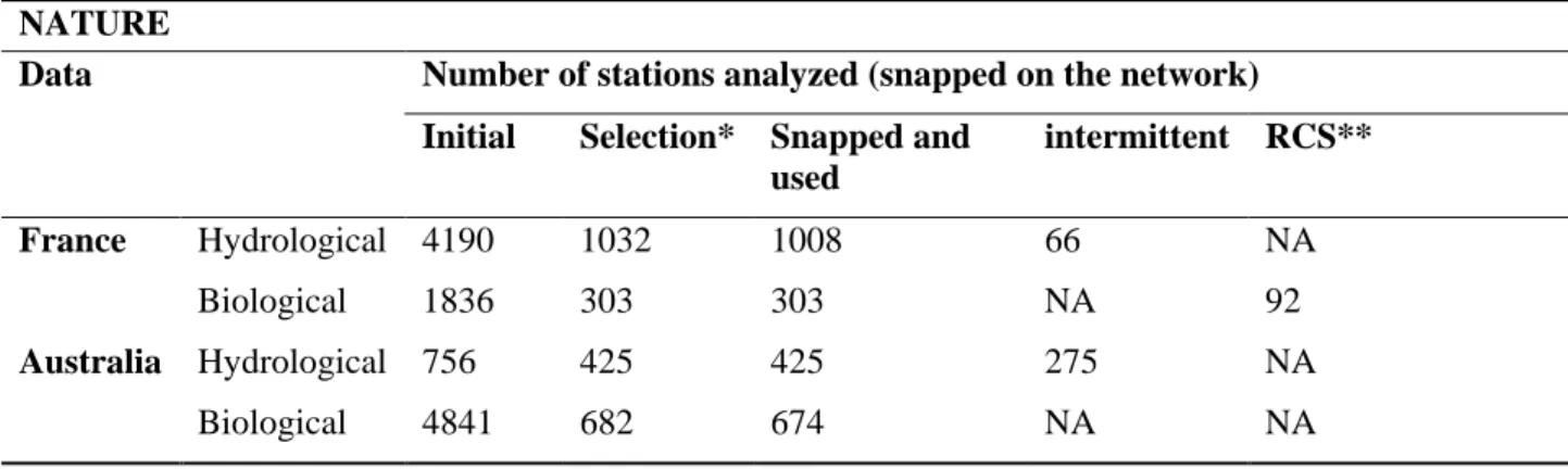
Table 3: Number of stations and nature of samples from the initial dataset (NA=Not applicable) NATURE

Data Number of stations analyzed (snapped on the network) Initial Selection* Snapped and

used intermittent RCS** France Hydrological 4190 1032 1008 66 NA Biological 1836 303 303 NA 92 Australia Hydrological 756 425 425 275 NA Biological 4841 682 674 NA NA

Table 4: Number and nature of available bio-monitoring

Macro-invertebrates Diatomates Macrophytes fish

France 301 301 246 247

Australia 674 NA NA NA

Table 5: Number and nature of selected stations *Selection and status of selected stations

Type of status Period of sampling Duration of sampling Missing data toleration Frequency of sampling France Hydrological T. Snelder’s

criteria 1970-2013 30 years <5% Automatic Biological “Referenced” = No human Pressure 1998-2001 2007-2011

2 years NA 1/ year max

Australia Hydrological T. Snelder’s criteria (Figure 4) 1970-2013 30 years <5% Automatic Biological AusRivAs protocol(reference condition sites only)

(31)

24

Quitterie Blanchard Final dissertation for an engineer degree 2014 By the end of this step of pre-selection, the set available for the next stage is based on the selection made according to the characteristics of the data for each station. For instance, the biological French network is composed of “referenced” stations, a term which required the samples to be extended to a certain amount of time, and the stations must be located in an area exempted from any kind of anthropic pressure.

At this stage, the set of data used in the study can be summarized in Table 6.

3. First decisions of sorting

In order to match (“couple”) the hydrological and biological stations, the criteria used to decide whether any two sites were appropriate to couple needed to be determined. After a quick discussion, the most obvious criteria to consider appeared to be the distance between stations from the hydrological network and stations from the biological network. This essential parameter could be analyzed in two different ways.

First, the Euclidian distance could be considered among each station, to define couples suitable to link as they belong to the same area. Then, thanks to the process of snapping the stations to a geo-localized network of flow path, the other tool used to build couples might be the linear length which separates two stations could be evaluated. At this stage, the distance was established as the first way to connect the stations.

This flow path distance was considered more appropriate than the Euclidian distance because the later method may associate some stations which do not belong to the same watershed, implying some significant differences between the stations, and may also induce the creation of couples between intermittent and perennial sites.

To avoid this, other variables besides distance were also considered and selected: altitude and drainage area, assuming that two stations with comparable values of surface drained would be likely to produce a suitable match. Indeed, in a similar nature of climate, it appears that the discharge in a catchment point is correlated to the surface of the watershed, and that governs the hydrological behavior of the site.

An equation was defined, in order to associate sites with similar parameters, linking data from both the biological network and the hydrological one:

Table 6: Final number of stations used

Biological sites Hydrological sites

Total Perennial intermittent

France 303 1008 942 66

(32)

25

Quitterie Blanchard Final dissertation for an engineer degree 2014 Equation 1: Appreciation of the difference

| | With:

: The surface drained at the biological station.

: The surface drained at the hydrological station.

This means that using this selection prevents the coupling of stations which do not have an absolute difference of surface drained higher than 25% of their average value. In that way, the stations which are linked together are more likely to share a comparable hydrological regime.

II. Concrete methods and tools used

1. ARCGIS and the distance study 1. Buffer zone

In order to be able to consider the distances between the stations, it is naturally essential to use a Geographic Information System, so that the stations can be localized on a map and different measurement can be evaluated. Indeed the latitude and the longitude were available in the data set, and allowed to start the calculations.

Indeed, the GIS software edited by ESRI was needed for this study. ARCMAP 10.2 is able to represent any given point on the Earth’s, using a specified projection. ARCGIS provides a significant range of tools in order to be able to manage, analyze of even visualize the considerate data (Esri).

This preliminary work leads to a basic sort, giving a primary idea about the available data set. Those results, accessible for France, can be summarized in Table 7.

As a first step, this software allows to estimate distances as the crow flies, between the two kinds of station. ESRI’s software can actually furnish an analyzing tool which can realize a matrix representing all the possibilities to link two groups of stations, in that case, hydrological and biological sets, within a chosen distance, based on their location on the map. This measurement, carried out for France in this part is presented in Table 7 .

(33)

26

Quitterie Blanchard Final dissertation for an engineer degree 2014 Table 7: Possible coupling results for France between 303 biological stations and 1008 hydrological

stations including 66 intermittent ones.

Number of potential couples between the 303 biological stations and hydrological stations

Distance All hydrological stations(1008) Intermittent hydrological stations(66)

<2km 21 1 <5km 53 1 <10km 173 5 <20km 483 18 <30km 682 30 <50km 893 42

2. Method to assess the length of the flow path between two stations

Considering the length of the flow path between two stations seems to be, at first sight, the most promising way to reach usable pairs of data. As the dataset is updated, projected, localized and ready to be used in ARCGIS, the issue consisted in finding the most effective tool to evaluate these distances.

To reach these results, some functions are usable in ARCGIS but require some data management, such as converting the layer into a network dataset, to be able to apply the tools provided. The flow paths are assimilated to roads and allow the analyses required.

An “OD cost matrix” was calculated, providing a “cost” information about the route linking an Origin location to a Destination. The “cost” appellation refers to the pressure, the constraint associated to the route. Considering that the length of the flow path which separates the two locations as a constraint to the travel, allows to assimilate the “cost” to the distance between an Origin and a Destination. Then, the biological network of stations was saved as Origin locations, and finally, the hydrological set represented the Destination to look for. Concerning the analysis options, they were picked in order to provide a matrix associating for each biological station ID, the ID of each connected hydrological station, the linear distance between them, and the destination rank, with a sort based on the proximity.

To avoid lengthy processing times, only ten hydrological destinations maximum were allowed to be linked to each biological station. So the function was looking for the 10 closest Destinations from an Origin, and applied the function to the next origin.

This method was applied to France (Figure 5) and Australia, and analyses can be summarized in this plot, which sort, the potential couples depending on the linear distance between them (Table 8).

(34)

27

Quitterie Blanchard Final dissertation for an engineer degree 2014 Table 8: Linear distances among biological and hydrological stations in France and in Australia

Linear distance Type of station Nature of information France Australia

< 5km

All stations Number of couples 31 72

Unique station involved 31 69

Intermittent Number of couples 1 41

< 10km

< 15km

< 20 km

<50 km

Intermittent

Number of couples 19

Unique station involved 14

<100 km Number of couples 70

(35)

28

Quitterie Blanchard Final dissertation for an engineer degree 2014 Figure 5: Localization of couples between intermittent hydrological stations and biological stations from the RCR within 50km

At first sight, the difference between the two countries is compelling. Indeed, even if the total number of Australian stations is higher than for the French stations, there is a pronounced imbalance among perennial and intermittent stations in France. At this stage, it was evident that the model built analyzing the stations would not be the same for the two countries, and it explains why, for France, a qualitative sort, attributing less weight to the linear distance was considered.

Therefore it was decided to use two separate methods of analyses to select the couples for France and Australia.

2. France

1. Qualitative selection applicable for the French dataset

According to the first visualization of the data, the criteria of distance, applied for France seems too restrictive (Figure 5), and some different sorts mentioned previously had to be reconsidered. As a matter

(36)

29

Quitterie Blanchard Final dissertation for an engineer degree 2014 of fact, even if the distance seemed obviously the most pertinent classifying parameter, R (R Development Core Team) and ARCGIS (Esri) were used to sort the stations according physical characteristics, the drainage area and the altitude, that were both available for almost all the hydrological and the biological stations.

The data needed to be comparable, even though the measurements were not homologues from the biological protocol to the hydrological network of stations. Thus, the information was collected from the same entity, the RHT, involving a tool in ARCGIS, able to associate to each station the data of the stream segment they were connected with.

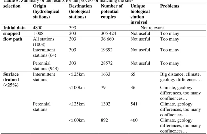
Hence, in this part of the study, the distance is ignored, and all the attention is focalized on the parameters mentioned previously, the surface drained and the elevation (e.g. Table 9). In this aim, every combination is examined, no matter how far the stations are from each other. This method, which was not considered at first as relevant, because it involved the comparison of two stations from different watershed, will be used for France only, to find alternative ways to get round the problem of the lack of couples identified for intermittent sites.

Table 9: Summary of the results for the process of matching the sites selection Origin (hydrological stations) Destination (biological stations) Number of potential couples Unique biological station involved Problems

Initial data 4800 393 Not relevant

snapped 1 008 303 305 424 Not useful Too many

flow path All stations (1008)

303 36 660 Not useful Too many

Intermittent stations (64)

303 19392 Not useful Too many

Perennial stations (943)

303 28572 Not useful Too many

Surface drained (<25%)

Intermittent stations

<125km 1633 65 Big distance, climate,

geology differences…

<100km 79 36 Climate, geology

differences, too many confluences… Perennial

stations

differences, too many confluences…

Even though the acceptable number of couples that emerge from this selection (Table 9), it was finally decided that the French data could not be used to build a model of flow relationships in intermittent rivers using the actual monitoring network datasets. Indeed, the significant distance separating the stations