Developing hydrogeophysics for critical zone studies, importance of heterogeneities and processes at the mesoscopic scale

(1)

HAL Id: tel-02865330

https://hal.archives-ouvertes.fr/tel-02865330

Submitted on 11 Jun 2020

HAL is a multi-disciplinary open access

archive for the deposit and dissemination of sci-entific research documents, whether they are pub-lished or not. The documents may come from teaching and research institutions in France or abroad, or from public or private research centers.

L’archive ouverte pluridisciplinaire HAL, est destinée au dépôt et à la diffusion de documents scientifiques de niveau recherche, publiés ou non, émanant des établissements d’enseignement et de recherche français ou étrangers, des laboratoires publics ou privés.

Developing hydrogeophysics for critical zone studies,

importance of heterogeneities and processes at the

mesoscopic scale

Damien Jougnot

To cite this version:

Damien Jougnot. Developing hydrogeophysics for critical zone studies, importance of heterogeneities and processes at the mesoscopic scale. Geophysics [physics.geo-ph]. Sorbonne Université, 2020. �tel-02865330�

(2)

SORBONNE UNIVERSITE Faculté des Sciences et Ingénierie

Dossier scientifique présenté en vue de l’obtention de L’HABILITATION A DIRIGER DES RECHERCHES

DEVELOPING HYDROGEOPHYSICS FOR CRITICAL ZONE STUDIES,

IMPORTANCE OF HETEROGENEITIES AND PROCESSES AT THE

MESOSCOPIC SCALE

Par

Damien JOUGNOT

Soutenue le Vendredi 17 janvier 2020, devant le jury

Colette SIRIEX Professeur, Université de Bordeaux Rapporteur

Frédéric NGUYEN Professeur, Université de Liège Rapporteur

Jean-François GIRARD Professeur, Université de Strasbourg Rapporteur

Linda LUQUOT Chargée de Recherche, Université de Montpellier Examinateur

(3)

List of Figures

1.1 Evolution of the number of publications with the topic “Critical Zone” in Web of

Science (search results obtained on March 11, 2019). . . 10

1.2 Replacing the critical zone at the center of the attention: (a) classical view of the globe and (b) anamorphosis that places the layers that are really critical for life on Earth in the center (Arènes et al., 2018). . . 11

1.3 Distribution of the CRITEX work packages (Gaillardet et al., 2018). . . 12

1.4 Overview of geophysical methods used and developed in the ENIGMA ITN (enigma-itn.eu): (a) general view, (b) from surface to boreholes, (c) cross holes, and (d) at the small scale (Credits: ENIGMA ITN). . . 13

2.1 Principle of the Time Domain Induced Polarization method (from Ghorbani, 2007). . 16

2.2 Principle of the Spectral Induced Polarization method (from Ghorbani, 2007). . . 16

2.3 Principle of geoelectrical imaging (from Binley and Kemna, 2005). . . 17

2.4 Principle of the Self-Potential measurement (from Darnet and Marquis, 2004). . . 18

2.5 Principle of seismic refraction acquisition (Credits: M. Dangeard). . . 19

2.6 Principle of the Seismo-Electrical measurements (from Holzhauer and Yaramanci, 2011). . . 20

2.7 The importance of scales in critical zone studies (modified from Hubbard and Linde, 2011). . . 21

2.8 Identification of the mesoscale. . . 22

3.1 (a) Sketch and (b) picture of the millifluidic geoelectrical set-up used in Jougnot et al. (2018). It corresponds to the set-up proposed by Jiménez-Martínez et al. (2015) that we adapted to monitor electrical conductivity in the flow cell during a tracer test experiment. . . 25

3.2 (a) Evolution of the electrical resistivity during the tracer test under fully saturated conditions. (b-e) four snapshots of the percolation of the tracer in the flow cell (from Jougnot et al., 2018). . . 26

3.3 (a) Evolution of the electrical resistivity during the tracer test under partially saturated conditions. (b-e) four snapshots of the percolation of the tracer in the flow cell (from Jougnot et al., 2018). . . 27

3.4 (a and c) Normalized tracer concentration and (b and d) current density spatial distri-bution between the potential electrodes at a late stage of the tracer test experiments under saturated and partially saturated conditions (from Jougnot et al., 2018). . . 28

3.5 Schematic of the flux-averaging upscaling procedure to obtain the effective excess charge density in a porous medium. . . 29

3.6 (a) Sketch of the EDL at the pore scale. Distribution of (b) the excess charge and (c) pore water velocity in the pore water as function of the distance to the shear plane (from Jougnot et al., 2020). . . 30

3.7 Drying of a bundle of capillaries, the larger pores are the first to be drained as the capillary pressure increases. . . 31

(6)

3.8 Evolution of the effective excess charge density as a function of water saturation for various soil types using the (a) WR and the (b) RP approaches (from Jougnot et al., 2012). The hydrodynamic parameters of the 12 types of soil are the one proposed by Carsel and Parrish (1988). . . 31 3.9 Evolution of effective excess charge density with salinity (from Jougnot et al., 2020). 33 3.10 Evolution of effective excess charge density with the permeability (from Jougnot

et al., 2020). . . 33 3.11 Comparison between the models of Linde et al. (2007), Jougnot et al. (2012) (WR

and RP appraoches) and the one proposed by Soldi et al. (2019) for four type of soils: (a) loam, (b) loamy sand, (c) sand, and (d) sandy loam (from Soldi et al., 2019). . . . 34 3.12 (a) 2D Pore network used to compute the effective excess charge density for four

types of PSD: (b) fractal, (c) exponential symmetric, (d) lognormal, and (e) double lognormal (modified from Jougnot et al., 2019). . . 35 3.13 (a) Electrokinetic coupling coefficient and (b) effective excess charge density from

the pore network simulations (from Jougnot et al., 2019). . . 36 3.14 Effective excess charge density exctracted from the SP signal measured in Doussan

et al. (2002) as a function of saturation during an (a) infiltation and (b) drainage phase of the event. Comparison of these data with the numerical WR and RP approaches of Jougnot et al. (2012) and the analytical closed form equation of Soldi et al. (2019) at three salinities (figure from Soldi et al., 2019). . . 37 3.15 (a), (b), and (c) location of the Volund agricultral test site and lateral and vertical

distribution of the instrumentation therein. (d) Measured and simulated SP signal as a function of depth prior to the tracer infiltration. Comparison between the prediction of the existing effective excess charge model from Linde et al. (2007) and the two approaches from Jougnot et al. (2012) (modified from Jougnot et al., 2015). . . 38 3.16 Numerical simulation of (a) the Darcy velocity, (b) tracer saline concentration, (c)

SP electrokinetic and (d) electrodiffusive contributions as a function of depth before and after the saline tracer injection at the Voulund agricultural test site (from Jougnot et al., 2015). . . 39 3.17 (a) SP monitoring set-up around the Douglas-fir tree at the in the H.J. Andrews

Exper-imental Forest. (b) Measured and (c) simulated SP signals from eco-hydro-electrical coupled model (modified from Voytek et al., 2019). . . 40 3.18 Evolution of the diel SP signal measured close to the tree roots (modified from Voytek

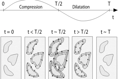
et al., 2019). . . 41 4.1 Illustration of the concept of Wave Induced Fluid Flow (from Müller et al., 2010).

Arrows indicate the fluid flow direction. . . 43 4.2 (a) Oscillatory compressibility test to simulate WIFF. Numerical simulation results for

the (b and c) horizontal and (d and e) vertical components of the maximum relative fluid velocity field. The results correspond to an oscillatory compressibility test at the frequencies of (b and d) 1 Hz and (c and e) 10 kHz. Modified from Jougnot et al. (2013). 45 4.3 (a and b) Electrical potential distribution and (c and d) resulting electrical potential

differences at two electrodes with respect to the reference electrode as functions of the normalized time. The grey square and the two circles (a and b) highlight the position of the reference and the potential electrodes, respectively. The results correspond to an oscillatory compressibility test at (a and c) 1 Hz and (b and d) 10 kHz (from Jougnot et al., 2013). . . 46 4.4 Effect of background permeability upon (a) the amplitude and (b) the phase of the

electrical voltage recorded at the top electrode (y = 2.5 cm in Fig. 4.3) for different frequencies (from Jougnot et al., 2013). . . 46

(7)

4.5 Numerical 2D rock samples used to test the effect of fracture connectivity on the seis-moelectric signal: (a) sample containing horizontal fractures that are not connected between each other, (c) sample containing the same horizontal fractures as (a), plus vertical fractures, which are not connected to the horizontal ones, (e) sample con-taining the same amount of horizontal and vertical fractures as in (c) but with some of the fractures connected, and (g) same as (b) but with most of the fractures con-nected. (b, d, f, and h) Amplitudes of the electrical potential in the samples shown in the left column for a frequency of 0.73 Hz. (i) Calculated total energy converted to seismoelectric signals at the sample scale. Modified from Rosas-Carbajal et al. (2019). 48 4.6 (a) Configuration used to validate the modeling approach of Roubinet et al. (2016)

where the red cross represents the position of the considered pumping well. (b and c) Spatial distribution of the SP signal computed with the DDP approach where the white square represents the position of the reference electrode. (d and e) Polar plots of the SP signal with respect to a reference located at the black cross in b and c, respectively, and computed with the DDP approach (blue lines) and a finite-element solution (red crosses). Note that matrix fluid flow was ignored in b and d and accounted for in c and e (from Roubinet et al., 2016). . . 50 4.7 (a-c) Studied fractured domains where the red cross represents the position of the

considered pumping well. (d-f) Spatial distribution of the SP signal with respect to a reference electrode located at position (x,y)=(0,0). (g-i) Polar plots of the SP signal along the dashed white circle plotted in (d-f) with respect to the minimum value measured along this circle and represented with a white cross. From Jougnot et al. (2020). . . 51 5.1 Schematic description of the system under consideration. (a) Stratified front between

species A and B that can be considered as a superimposing individual shear flows. Based on the direction of the applied potential difference to simulate an electrical conductivity measurement with respect to the shear flow, the three studied are dis-tinguished: (b) parallel configuration (i.e., parallel to the flow direction), (c) mixed configuration (i.e., perpendicular to the flow direction but parallel to the plane of shear), and (d) normal configuration (i.e., perpendicular to both the flow direction and the plane of shear) (from Ghosh et al., 2018). . . 53 5.2 (a) Evolution of the relative change in effective conductivity with time, for the three

configurations (i.e., its anisotropy). (b-d) Spatial distribution of product concentration (normalized by the initial reactant concentration) at three different times (from Ghosh et al., 2018). . . 54 5.3 Effect of transport parameters on the effective conductivity for the three

configura-tions: (a, b, c) Péclet (Pe) and (d, e, f) Damköhler (Da) numbers. For all cases, the effective electrical conductivity initially follows the trend observed in the absence of velocity gradients (P e = 0) (from Ghosh et al., 2018). . . 55 5.4 (a) Basic Stern interface model to describe the calcite-water interface (calcite (1 0 4)

surface) when calcite is in contact with a NaCl and CaCl2aqueous solution at equilib-rium with a pCO2. (b) Sketch of the complex conductivity model of the experiment of Wu et al. (2010): precipitation of calcite on glass beads. Calcite particles that are mostly rhombohedral, are approximated as spheres. Modified from Leroy et al. (2017). 56

(8)

5.5 Imaginary conductivity spectra of calcite precipitation on glass beads as a function of time in days (a) before and (c) during the pore clogging by the calcite precip-itate. Imaginary conductivities inferred from the complex conductivity model are represented by the lines and the symbols represent the imaginary conductivity mea-surements of Wu et al. (2010). (b) and (d) evolution of the computed calcite particle size distribution of during calcite precipitation corresponding the model of (a) and (c), respectively. Modified from Leroy et al. (2017). . . 57 5.6 Computed particles cementation exponent (m) and formation factor (F) changes

dur-ing the calcite precipitation experiment of Wu et al. (2010). The cementation expo-nent and formation factor of the glass beads pack where calcite precipitation occurs have a different trend of changes before and after the starting of the pore clogging (day 9) (from Leroy et al., 2017). . . 58

5.7 Sketch of the proposed approach for the GeoProcesS project: coupling geophysical

and biogeochemical methods to study bioremediation processes. . . 59 5.8 Sketch of the different compartments in the critical zone (from Chorover et al., 2007). 60

(9)

Foreword

This HDR manuscript synthesizes the research that I have been conducting during the last ten years (i.e., since the my PhD defense): during 5 years at University of Lausanne as a post-doc in the group of Niklas Linde and during 5 years at UMR 7619 METIS, Sorbonne Université, as a CNRS researcher. These investigations are the result of a collective work in close interaction with PhD students, post-docs, and researchers in my labs but also abroad. Indeed, in addition to my host institutions, I had the chance build up a network of fruitful national and international collaborations (Argentina, Belgium, Denmark, France, Germany, Spain, Switzerland, United States). The main part of this document con-sists in the HDR thesis, followed by personal information (CV, publications, student mentoring), and a selection of five representative publications.

(10)

Abstract

The critical zone is the thin outer layer supporting life on earth. It is a compartment in which many complex and coupled bio-chemico-physical processes take place. Characterizing and monitoring these processes is of utmost importance to understand and protect the critical zone. Geophysical methods are very appropriate tools to study them in situ and non-intrusively thanks to the sensitiv-ity of measurable physical parameters to properties of interest. However, the critical zone is also a very heterogeneous medium at different scales and the quantitative use of geophysics rely on our capability to take them into account effectively. In this manuscript I present the various works that I conducted during the last ten years to better use hydrogeophysical methods by taking heterogeneities into account: from theoretical petrophysical model developments to laboratory experiments and in situ monitoring in critical zone observatories. After presenting the geophysical methods I have been using, I define the concept of mesoscopic scale heterogeneities, that is: larger than the pore scale but smaller than the resolution of the considered geophysical method. The first heterogeneities that I present are related to the pore size distribution and its impact on the water saturation, flow and solute transport properties. The second heterogeneities that I study are the presence of fractures and fracture networks in porous media. The final kind of heterogeneities that I am considering are induced by local biogeochemical reactions and their impact on geophysical signals. These new advances and on-going research projects pave the way to a more quantitative and more integrated use of geophysics to study the critical zone in its true complexity.

(11)

Résumé

La zone critique est la fine pellicule externe qui permet la vie sur terre. C’est un compartiment dans lequel ont lieu de nombreux processus couplés bio-chimio-physiques. La caractérisation et le suivi de ces processus sont d’une importance cruciale pour comprendre et protéger la zone critique. Les méth-odes géophysiques sont des outils tout particulièrement adaptés pour étudier ces processus in situ et de façon non-intrusive grace à la sensibilité des mesurables physiques aux propriétés d’intérêt de la zone critique. Toutefois, la zone critique est un milieu très fortement hétérogène aux différentes échelles et l’utilisation quantitative de la géophysique dépend de notre capacité à les prendre en compte efficace-ment. Dans ce manuscrit, je présente les différents travaux que j’ai menés durant les dix dernières années pour une meilleur utilisation de l’hydrogéophysique en prenant en comptes ces hétérogénéités: du développement de modèles pétrophysiques au expériences de laboratoire et aux suivi in situ dans des observatoires de la zone critique. Après une brêve présentation des méthodes géophysique que j’ai utilisées, je définis le concept d’hétérogénéités à l’échelle mésoscopique, c’est à dire plus grande que l’échelle porale mais inférieure à la résolution de la méthode géophysique considérée. Les pre-mières hétérogénéités que je présente sont liées à la distribution de taille des pores dans le milieu et son impact sur la saturation en eau, le flux d’eau et le transport de solutés. La deuxième sorte d’hétérogénéités que j’étudie est la présences de fractures en milieu poreux et de réseaux de frac-tures. Le dernier genre d’hétérogénéité que je considère est induit par des réactions biogéochimiques à l’échelle locale et leur impact sur les signaux géophysiques. Ces nouvelles avancées et les projets de recherche que je mène actuellement ouvrent la voie à une utilisation plus quantitative et intégrée de la géophysique pour l’étude de la zone critique dans toute sa complexité.

Mots clés: Zone critique, Hydrogéophysique, Milieux hétérogènes, Pétrophysique, Changement

(12)

Chapter 1 Introduction

The Critical Zone has first been defined by the US National Research Council in 2001 as the first research opportunity for the near future.

“The Critical Zone: [an] heterogeneous, near surface environment in which complex

interactions involving rock, soil, water, air, and living organisms regulate the natural habitat and determine the availability of life-sustaining resources.” (NRC, 2001)

And a shorter definition of the critical zone could be the earth skin: “from the top of the canopy down to the base of the groundwater zone”. Since then, the critical zone has been the subject of an increasing number of scientific studies and publications (Fig. 1.1).

Figure 1.1: Evolution of the number of publications with the topic “Critical Zone” in Web of Science (search results obtained on March 11, 2019).

Critical zone studies are truly trans-disciplinary by nature as they cross so many scientific research areas in geosciences. The “critical” importance of this zone to human societies and life on earth in general is generating researches of more philosophical nature, such as Arènes et al. (2018) recently proposed to replace the critical zone “at the center of the attention” given the various environmental issues that the human species will have to face in the near future (Fig. 1.2).

Studying the critical zone Better understanding the critical zone is also a matter of research strate-gies in which overlap observation, modeling, and process studies in controlled environments. Critical zone observatories and networks exist in different countries across the world. In France the study of the critical zone is mainly done through two main initiatives: OZCAR (Observatoires de la Zone Critique Application et Recherche or Critical Zone Observatories - Application and Research, see www.ozcar-ri.org) and CRITEX (challenging equipment for the temporal and spatial exploration of

(13)

Figure 1.2: Replacing the critical zone at the center of the attention: (a) classical view of the globe and (b) anamorphosis that places the layers that are really critical for life on Earth in the center (Arènes et al., 2018).

The three main scientific research orientations and open questions for critical zone studies through the OZCAR test site network are:

• Dynamic architecture of the Critical Zone: What is the vertical and lateral extent of the Critical Zone? What are the residence and exposure times of water and matter in the different compartments? What are the critical zone interfaces? what are the important critical zone interfaces? What is the role of biota in the Critical Zone?

• Biogeochemical cycles, sediment and/or contaminant propagation through the critical zone from highlands to sea: Can we better quantify budgets of mass and energy across our critical zone observatories? How high frequency sampling can help deciphering critical zone functioning? What is the functional role of biota?

• Responses and feedbacks to biological, climatic and geological perturbations and global change. The Earth’s surface dynamic system: How can we use observatories to predict the future of the critical zone? How do processes with small characteristic time and limited spatial

(14)

imprint influence the longer time-scales and larger spatial scales? Can we predict critical zone trajectories?

In order to answer to those questions, the French project CRITEX has been funded to acquire or develop adequate equipments to perform a state-of-the-art temporal and spatial exploration of the critical zone. The different work-packages of CRITEX focus on two main challenges: to be able to perform high frequency measurements and to study in detail hot-spots and hot-moments (Fig. 1.3).

Figure 1.3: Distribution of the CRITEX work packages (Gaillardet et al., 2018).

Using geophysical tools to study the critical zone One can see that geophysical tools are well represented in the work-packages of the CRITEX project and it is the kind of tools that I decided to work on and develop. Indeed, if geophysical methods have been previously developed for mining and oil & gas reservoir applications, their sensitivity to parameters and processes of interest make them essential to study the critical zone. During the last two decade a new discipline is emerging: the hydrogeophysics. The American Geophysical Union (AGU) Hydrogeophysics Technical Committee, upon which I am a member since 2015, proposes the following definition:

“Hydrogeophysics involves use of geophysical measurements for estimating parameters and monitoring processes that are important to hydrological studies, such as those associ-ated with water resources, contaminant transport, ecological and climate investigations. Improved characterization and monitoring using hydrogeophysical techniques can lead to improved management of our natural resources, understanding of natural systems, and remediation of contaminants.” (http://hydrogeophysics.org/)

Hydrogeophysics as a discipline has been the subject of many books (e.g., Rubin and Hubbard, 2005; Vereecken et al., 2006), book chapters (e.g., Hubbard and Linde, 2011), and review papers (e.g., Binley et al., 2015; Parsekian et al., 2015) over the years. This discipline starts to be pretty established in the critical zone research community, and there is a real need for the formation of a new generation of scientists to correctly use and push further the development of these tools. This yields

(15)

https://cargese2018.sciencesconf.org/), and Innovative Training Network (ITN) at the European scale (i.e., the ENIGMA ITN), that are oriented towards hydrogeophysics.

Among other initiatives, the ENIGMA ITN, for European training Network for In situ imaGing of dynaMic processes in heterogeneous subsurfAce environments, is funded by the Marie Sklodowska-Curie action grant of the European Union’s Framework Programme for Research and Innovation H2020 (https://enigma-itn.eu/). Its goal is to train a new generation of 15 young researchers in the development of innovative methods for imaging process dynamics in subsurface hydrosystems, in order to enhance understanding and predictive modelling capacities and to transfer these innovations to the economic sector (Fig. 1.4). The 15 young future PhD students will contribute to develop the spatial representation of subsurface heterogeneity, fluxes, chemical reactions and microbial activity, through the integration of data and approaches from geophysics, hydrology, soil physics, and bio-chemistry. The network ENIGMA gather 21 partners (15 academic and 6 industrial) from 8 European countries. The Enigma ITN started in January 2017 and will run until December 2020, I serve as deputy coordinator of the project.

Figure 1.4: Overview of geophysical methods used and developed in the ENIGMA ITN (enigma-itn.eu): (a) general view, (b) from surface to boreholes, (c) cross holes, and (d) at the small scale (Credits: ENIGMA ITN).

As hydrogeophysics attracts an increasing number of users in the research community due to its interest to study the critical zone, many limitations start to be unveiled, generating motivation for new researches, inducing theoretical and technical developments. First, the geophysical instrumentation has been drastically improved over the last two decades, providing user friendly tools with faster acquisition (i.e., multi-channel acquisition) and better accuracy. Then, inversion algorithms and

(16)

in-creasing computing power is allowing paradigm changes in imaging strategies (i.e., joint inversion approaches) and uncertainty characterization (i.e., from deterministic to stochastic inversion). Fi-nally, more theoretical investigation, such as physical and mathematical developments or laboratory works, are continuously improving our understanding of how the measured geophysical signal is gen-erated by state properties or processes of interest in critical zone studies: namely the petrophysical relationships.

In the present document, I propose a synthesis of the works I have been conducting since my PhD defence in 2009 to improve the way we use hydrogeophysics. Most of it falls under that third topic, that is developing and testing new or better petrophysical relationships. In a nutshell, my work of the last decade could be summarized by the following question: how to better take into account heterogeneities in the geological media at the mesoscopic scale in the generation of geophysical signals for hydrology and critical zone studies ?

The first chapter will present some theoretical bases such as: the principles of the different geo-physical methods I have been using and developing and the definition of what does mesocopic scale refer to in hydrogeophysics. In the second chapter, I will present the work related to mesoscopic heterogeneities under partial saturation and its impact on water flow and transport properties. In the third chapter, I will present my work related to fractures and fracture network and how they affect geophysical signatures. The fifth chapter then deals with a field that I am just starting to explore, the influence local heterogeneities related to biogeochemical reactions. The last chapter is dedicated to some conclusion on these works and outlook for future ones.

(17)

Chapter 2 Methods and definitions

Geophysics covers a large range of research areas using a large variety of tools (relying on different physical principles) at various scales (from the pore to the entire earth). Geophysical measurements can be made from the surface or within a geological medium, but also on samples in laboratory conditions. They are generally considered to be not (or less) intrusive and less expensive than most other techniques (i.e., drilling, excavation). They also present the big advantage to be repeatable (e.g., time-lapse) and therefore allow the monitoring of state changes of the geological target.

The present chapter is restricted to only a couple methods that can be used to study the critical zone: the one I used and/or developed while conducting my research during the last decade. This short presentation is therefore not exhaustive.

2.1 Presentation of the considered geophysical methods

2.1.1 Electrical resistivity and induced polarization

Electrical resistivity and induced polarization represent a familiy of active geoelectrical technics that have been discovered by the Schlumberger brothers a century ago: in 1912 for the Direct Current (DC) resistivity (Schlumberger, 1912) and in 1920 for the Induced Polarization (IP) effect (Schlumberger, 1920). As presented in detail by Binley and Kemna (2005), one can identify three different methods:

• DC resistivity

• Time Domain Induced Polarization (TDIP)

• Frequency Domain or Spectral Induced Polarization (SIP)

Electrical resistivity The measurement of the DC resistivity relies on Ohm’s law, it consists in injecting an electrical current in a geological medium and measure the resulting electrical potential differences to determine its electrical resistivity (or its reciprocal, the electrical conductivity). The electrical conductivity of a medium is strongly affected by key properties such as (for a review, see Glover, 2015): texture and structure (e.g., porosity, pore connectivity, fracturation), the lithology (e.g., the clay content), fluid saturation (e.g., water saturation), the pore water chemical compositions (e.g., salinity). During my PhD thesis, I worked on petrophysical relationships to relate the electrical conductivity with different transport properties such as the ionic diffusion coefficient (Jougnot et al., 2009), the thermal conductivity (Jougnot and Revil, 2010), or the hydraulic conductivity in partially saturated conditions (Jougnot et al., 2010b).

(18)

Induced polarization Induced polarization measurements can be divided in two approaches: time domain and frequency domain measurements. In IP measurements, dielectric phenomena (i.e. po-larization) are also taken into account. It is part of the low frequency electro-magnetic methods. Therefore, the property of interest is not only the resistivity, but rather the complex resistivity (or impedance).

Figure 2.1 illustrates the principle of TDIP measurements. Similarly to DC resistivity, a current is injected in a medium to obtain its electrical resistivity. But, when the current injection is stopped, the relaxation of the electrical potential differences is also measured. Monitoring this decrease is a way to determine how fast the medium de-polarize, that is to obtain its chargeability.

Figure 2.1: Principle of the Time Domain Induced Polarization method (from Ghorbani, 2007). Figure 2.2 presents the principle of SIP measurements. In this case, the current is injected using a sinusoidal function with a given frequency (Fig. 2.2a) and the resulting voltage is measured. This resulting voltage also has a sinusoidal shape with a different amplitude and a phase lag. The electrical resistivity is obtain from the amplitude and Ohm’s law, while the phase, usually negative, is related to the chargeability of the medium. By sweeping this measurements over a large range of frequencies, typically from 1 mHz to 10 kHz, one can obtain the amplitude (i.e., resistivity) and phase (i.e., related to the chargeability) spectra of the complex resistivity (Fig. 2.2b).

Figure 2.2: Principle of the Spectral Induced Polarization method (from Ghorbani, 2007). Like the resistivity, the chargeability (or the phase) of a geological medium can be related to many parameters of interest such as: the clay content (through the cationic exchange capacity), the fluid phase composition (e.g., water saturation, presence of pollutant, chemical composition). During my PhD thesis I did study the effect of the clay rock dessication on several parameters obtained by

(19)

part of the polarization phenomena (Jougnot et al., 2010a). Many works on TDIP or SIP try to relate the chargeability or phase information to predict the permeability of porous media (e.g., Revil and Florsch, 2010; Zisser et al., 2010).

These DC resistivity and IP measurements can be on sample using a fixed measurement set-up or they can be displaced to image geological media. This imaging technique is called Electrical Resistivity Tomography (ERT) for DC measurements and Electrical Impedance Tomography (EIT) for IP measurements. The principle of electrical tomography from the surface is illustrated by Fig. 2.3. Displacing current and potential electrodes allow us to scan the subsurface and obtain apparent properties (i.e., apparent resistivity). Then, inversion algorithms can be applied to retrieve the “true” property distribution (resistivity and chargeability or phase) (e.g., Binley and Kemna, 2005).

Figure 2.3: Principle of geoelectrical imaging (from Binley and Kemna, 2005).

2.1.2 Self-potential

The Self-Potential (SP) is a passive geophysical method that consists in measuring the naturally oc-curring electrical field at the surface or within a geological medium. It is one of the oldest geophysical methods (see Fox, 1830).

The measurement principle of SP is rather simple one, as illustrated in Fig. 2.4, SP measurements can be done with only two non-polarizable electrode (e.g., Petiau, 2000) and a high impedance volt-meter. One can measure and represent it as SP profiles, 2D maps, 3D electrical field, or time series. However, as pointed by Susan Hubbard in the foreword of Revil and Jardani (2013)’s book on the SP method:

“Although self-potential data are easy to acquire and often provide good qualitative infor-mation about subsurface flows and other processes, a quantitative interpretation is often complicated by the myriad of mechanisms that contribute to the signal.” S. Hubbard The different sources generating SP signal can be divided in two kinds:

• Electro-kinetic: related to water flow (streaming potential)

• Electro-chemical: related to concentration gradient (diffusion or junction potential), thermal gradient(temperature potential), or redox gradients (redox potential)

These sources are additive and often superposed when measuring the electrical field. Their relative contributions to the total SP signal depends on the medium conditions and processes (e.g., Jouniaux et al., 2009; Revil and Jardani, 2013).

(20)

Figure 2.4: Principle of the Self-Potential measurement (from Darnet and Marquis, 2004). Electrokinetic contribution SP signals of electrokinetic nature have been studied since Quincke (1859) and quantified by modeling since Helmholtz (1879) and von Smoluchowski (1903). They are link to the presence of an Electrical Double Layer (EDL) at the interface between the mineral and the pore water, that is the presence of an excess of charge in the pore solution that counterbalance free charges at the mineral’s surface. When the water flows into the pores, it drags this excess charge, generating an charge separation and thus the so-called streaming current. These signals are usually referred to as Streaming Potential. During my PhD thesis, I started to work the mechanisms of these phenomena under partially saturated conditions (Linde et al., 2007; Revil et al., 2007).

Electro-diffusive contribution The presence of ionic concentration gradient in solutions yields to the diffusion of the ions towards smaller concentrations. When the ions do not have the same mobility an electrical current is generated to make them diffuse at the same velocity in order to respect the local electro-neutrality of the system. This phenomenon is also known as junction potential. In addition to this effect, the presence of electrical double layers, i.e, zones from where anions are partially or totally excluded can enhance of diminish this current generation. I worked on these phenomena in clay rocks during my PhD thesis (Revil and Jougnot, 2008; Jougnot et al., 2009).

Thermo-electric contribution When submitted to thermal gradient, ions also tend to diffuse as

their mobility strongly depends on the temperature. This phenomenon is described in details by Leinov and Jackson (2014).

Redox contribution This corresponds to the first application of the SP method, i.e., localizing ore bodies for the mining industry Fox (1830). When an electronic conductor (e.g., ore body, metallic pipe, bacterial nano-wires) connects two domains with different redox potential, it acts as a “geo-battery”, generating electrical current and electrical potential differences that can be significantly larger than the other contributions. It is important to note that if no electronic conductor connect the regions with different redox potentials, the electrical circuit is open and thus no electrical current nor electrical potential difference is generated.

The SP signal measured in natural media are therefore a superposition of potentially all these contributions. It is worth noting that the electrical resistivity of the geological medium has a strong influence on the amplitude of the SP signals. Hence it is crucial to determine the electrical resistivity of the medium in order to quantitatively approach the SP signal.

(21)

2.1.3 Seismic and seismoelectric methods

Over the course of my PhD thesis I mainly worked with the geo-electrical methods presented in the previous sections (i.e., SIP and SP), but during my post-doc at the University of Lausanne, I started to look into completely different, but yet complementary, methods based on wave propagation: seismic and seismo-electric methods.

Seismic methods Seismics methods are active geophysical methods based on the mechanical wave

propagation in the subsurface. A seismic acquisition set-up usually consist in a collection of geo-phones implanted along linear profiles or arrays, at the surface of the ground. The signal come from a seismic source generated by a portable mechanical source (often a hammer for near-surface appli-cations). Depending on the dimensions of the set-ups, the density of the arrays and the energy of the sources, the recorded wavefields can be analysed to image contrasts in mechanical properties of the near-surface (depths from 1 to 100 m, with resolution from 0.1 to 10 m-scale) using the standard equipments available for environmental applications. The most popular interpretation method is re-fraction tomography (Fig. 2.5) which consists in picking first arrivals times of the wavefield and then to invert for pressure (P) or shear (S) waves velocity models (VP or VS, depending on the type of sources and sensors). As an alternative to S-wave refraction tomography, the recorded wavefield can also be processed to extract surface-wave dispersion data that are then inverted for VS models (e.g., Pasquet and Bodet, 2017).

Figure 2.5: Principle of seismic refraction acquisition (Credits: M. Dangeard).

Seismic methods are becoming a common geophysical tool to study the Critical Zone. It was first applied to characterize the underground structures but now tends be more and more used to capture processes such as weathering (e.g., Clair et al., 2015), water content (e.g., Pasquet et al., 2016), or water redistribution (e.g., Dangeard et al., 2018). Indeed, P- and S-wave velocity can be related to the mechanical properties (i.e., density, porosity, fluid content) but also to textural and structural properties (e.g., lithology variation, presence of fractures). VP and VS show are not affect in the same way by saturating fluids, therefore VP/VS or Poisson’s ratio are usually estimated to identify them in porous media. However, the attenuation of the signal also carries interesting information regarding similar and complementary properties such as water content (Rubino and Holliger, 2012), medium permeability (Rubino et al., 2012), or fracture connectedness Rubino et al. (2013).

Seismoelectrical method The seismoelectric (SE) method relies on the measurement of an

(22)

of these signals dates back from Thompson (1936) and has been followed by many researches to propose theoretical frameworks explaining these signals during the last century (e.g., Frenkel, 1944; Pride, 1994; Pride and Garambois, 2005; Revil et al., 2015; Jouniaux and Zyserman, 2016).

The seismoelectrical conversion originates from electrokinetic coupling such as for SP signal generation, that is a charge separation due to a moving fluid along a charged surface: e.g., solid-solution (e.g., Leroy and Revil, 2004), air-solid-solution (e.g., Leroy et al., 2012). One can identify three kinds of seismoelectric signal (Fig. 2.6):

• The co-seismic signal: as the wave travels through the medium, it induces a relative displace-ment of the pore water along mineral surfaces, therefore a charge separation. This is the first identified SE signal in Thompson (1936). This signal travels with the wave and can only be detected as the wave reaches the array of measuring electrodes.

• The interface response: as the wave crosses some discontinuity in the medium, that is a con-trast in porosity, permeability, water content or any other property affecting the wave velocity, medium electrical conductivity, or excess charge density (see Mahardika et al., 2012, for a di-dactic example). This signal travels faster than seismic wave (i.e., electromagnetic wave) and is used to detect medium interface (e.g., lithology contrasts).

• The mesoscopic signal: this kind of signal is related to compressibility contrast at the meso-scopic scale along the wave path, it will be described in details in the chapter 4 (e.g., Jougnot et al., 2013).

(23)

2.2 Definition of the mesoscopic scale

2.2.1 Scales in critical zone studies

Scales are of tremendous importance in geosciences given the fractal nature of the world we live in (Maldelbrot, 1983). But when dealing with critical zone studies, this question of scales becomes even more crucial as features at the smallest scales can influence properties at the largest one (Fig. 2.7).

Figure 2.7: The importance of scales in critical zone studies (modified from Hubbard and Linde, 2011).

For example, mineral surface roughness and evolving pore space geometry (e.g., dissolution) affect water flow at the pore scale. The heterogeneity of these properties in turns results in preferential flows that can drive non-darcean or anomalous solute transport at larger scale making it difficult to model or predict contaminant transport at the human scale (drinking wells). Then, it can also drive flow pattern at catchment scales, generating a distribution of water saturation or erosion rate that can shape landscapes (geomorpholgy) or vegetation distribution (ecohydrology). Such analysis could be perform with any kind of heterogeneity or process of various disciplines such as physics, chemistry or biology.

Hydrogeophysical methods have a great interest for studying the critical zone as it provide physi-cal tools at all existing sphysi-cales. It goes from X-Ray imaging at the micrometer sphysi-cale to perform tomog-raphy of laboratory samples to gravity field measurements at kilometers scale for water distribution monitoring on the earth (i.e. GRACE). In between these two extreme scales, a lot of hydrogeophysical methods exist such as the one presented in section 2.1.

My work as mainly been focused on scales comprised between the nanometer (e.g., distribution of ions in the electrical double layer in Jougnot et al., 2009) to the kilometer (e.g., long ERT profile in

(24)

Gélis et al., 2010). The methods presented in section 2.1 have the great interest to be able to be used on geological media across circa 5 orders of magnitude of length scales (from 10−2 to 103 _{m), but} they suffer from limited resolution (e.g., Day-Lewis et al., 2005) that can’t be better than the sensors spacing or the wavelength (in the best case scenario).

2.2.2 Identifying the mesoscopic scale

Since my first research project during my master "Experimental and numerical study of hydraulic conductivity in partially saturated double porosity soils" (Jougnot et al., 2008), I mainly worked on heterogeneous media. Measurement responses always results from an integration over a certain volume. I will detail in the following chapters all the kind of heterogeneities I’m referring to (multiple porosities, cracks, fracture, partial saturation, chemical or energy gradients), but from all those works I could extract a common property: all my measurements where done at a resolution scale which was larger than the scale of the heterogeneity I was looking at. But it is only during my post doc that I came across the concept and a clear definition of the mesoscale.

The mesoscopic scale Müller et al. (2010) proposes a clear and simple definition of mesoscale or mesoscopic scale for seismic properties: it is the scale which is comprised between the pore scale and the measurement scale (Fig. 2.8). In seismic (and seismoelectric) methods the measurement scales depends on the wave length, but this concept can be used in all the other geophysical methods. Considering the electrical methods presented above (DC, TDIP, SIP, and SP), the measurement scale roughly correspond to electrodes spacing and its resolution decreases with the distance from those. In addition to the physical limitation of the measurements, one also has to account for resolution loss during the inversion/reconstruction process.

Figure 2.8: Identification of the mesoscale.

In hydrogeophysics, the measurement scale does not always correspond to a Representative El-ementary Volume (REV). Indeed, many contrasts in the structures, properties or processes existing at the mesoscopic scale affect the measurements in a way that cannot be easily described by an ef-fective property. Nevertheless, a single geophysical measurement can only produce a given datum. The challenge when dealing with mesoscopic heterogeneities is to link the measured signal to the heterogeneity or process that generates it.

The mesoscopic heterogeneities During the last decade, I have been studying different kind of

(25)

• Water distribution in saturated and partially saturated porous media: porous media usu-ally exhibit a certain heterogeneity in term of pore size distributions (PSD). From this meso-scopic heterogeneity result spatially distributed properties (e.g., porosity, permeability, water content) that can strongly affect flow and transport (e.g., preferential flow, non-darcean trans-port).

• Fractures and fracture networks in porous media: single fractures and interconnected frac-ture networks are probably one of the most contrasted kind of heterogeneities as it create strong local gradient in properties between the fracture and the matrix, also controlling flow and trans-port.

• Heterogeneities generated by transport and biogeochemical reactions: the critical zone is characterized by a large ranges of coupled processes of different nature (e.g., geochemical, biological). This reactivity also occurs with a certain spatial distribution in the medium: water and solute transport transport can either stop or reinforce these biogeochemical reactions by modifying local chemical and biological states (e.g., ionic concentrations, redox potentials, biochemical equilibrium).

(26)

Chapter 3 Water distribution in saturated and partially

saturated porous media

Partially saturated media are intrinsically heterogeneous as some pores are saturated by water while others are by gas (e.g., air) or by a non aqueous liquid phase (e.g., oil, organic contaminant). The spatial distribution of the water in porous media largely depends on the pore size distribution (PSD) (e.g., Bear, 1988) but can also depend on what happened to the medium (see Soldi et al., 2017, for an example about hysteretic effects). The porous medium structure and PSD can affect the water flow and transport distributions at the mesoscopic scale in both saturated and partially saturated conditions, but it is even more important under partially saturated conditions.

In this chapter, I present some of my works related to the effect of these heterogeneities on two main geophysical methods: electrical conductivity (section 3.1) and the self-potential (sections 3.2 and 3.3).

3.1 Effect of preferential flow and transport on electrical

conduc-tivity

3.1.1 Development of a millifluidic geophysical set-up

One of the main problems with studying rocks is to achieve non-destructive control of on-going processes. If geophysical methods are really powerful tools to monitor these, their integrative nature, the indirect measurements they provide and their limitations in term of resolution cannot allow to directly look into the studied media (see previous chapter).

During the last decades, increasing interest in milli- and micro-fluidic system have yield to tech-nical developments in many research fields, from physical to biological disciplines. de Anna et al. (2013) and Jiménez-Martínez et al. (2015) proposed interesting new millifluidic set-ups to study flow and transport in porous media. They developed a modified Hele-Shaw cell (i.e., two parallel glass plates separated by a very small aperture) by inserting vertical cylinders acting as obstacles for the flow and the transport: a 2D flow cell. Transport in the cell is monitored by a camera sensitive to the concentration of a fluorescent tracer in the pore fluid. The cell is designed to perform studies in two phase flow conditions (e.g., water and air).

In 2013, we adapted their millifluidic set-up by inserting copper electrodes in the flow cell in order to be able to monitor both the ionic concentration distribution at the microscopic scale with the camera (i.e., with several pixels per pore) and at the macroscale with the resistivity meter (i.e., one value for the entire cell). This experiment, presented by Jougnot et al. (2018), is, to the best of my knowledge, the first designed millifluidic geophysical set-up (Fig. 3.1). We used this set-up to monitor the saline tracer test in both saturated and partially saturated conditions.

(27)

Figure 3.1: (a) Sketch and (b) picture of the millifluidic geoelectrical set-up used in Jougnot et al. (2018). It corresponds to the set-up proposed by Jiménez-Martínez et al. (2015) that we adapted to monitor electrical conductivity in the flow cell during a tracer test experiment.

(28)

Figure 3.2: (a) Evolution of the electrical resistivity during the tracer test under fully saturated con-ditions. (b-e) four snapshots of the percolation of the tracer in the flow cell (from Jougnot et al., 2018).

3.1.2 Geolectrical monitoring of a saline tracer test at the mesoscopic scale

Prior to the saline tracer tests, we characterized the petrophysical properties of the flow cell, i.e., determining its formation factor and the saturation index from Archie (1942). This was done by sat-urating the cell homogeneously with a solution of a known concentration and electrical conductivity, then draining the cell to obtain partially saturated conditions. We repeated this procedure with differ-ent salinities to make sure that the surface conductivity of the material was negligible (see Fig. 4 of Jougnot et al., 2018).

We conducted the first tracer experiment under water saturated conditions. Saturating first the column with the background solution, prior to the injection of the saline tracer. Figure 3.2a shows the increase of the bulk electrical conductivity as the tracer percolate fairly homogeneously in the flow cell. As the saline tracer percolate in the medium, its becomes in contact with both potential electrodes (P1 and P2), creating a slow and progressive step increase in the effective electrical conductivity of the medium between t = 4000 s and 8000 s (Fig. 3.2a).

For the second tracer experiment, we established a partially saturated conditions with the back-ground solution prior to the tracer injection. It yields a much more complex geometry for its per-colation due to the presence of the air bubbles (in white in Fig. 3.2). As we inject the tracer at a constant flow rate, it percolates faster through the flow cell than under water saturated conditions, yielding a clear preferential flow (and electrical current) path (i.e., solute fingering). This results in a sharper step in the measured effective electrical conductivity (from t = 3000 s and 6000 s). Note that, as more tracer fingers connect the potential electrode, smaller steps are visible (t = 10000 s and t = 12000 s). Such preferential phenomena are well know in the literature on transport in porous media and particularly critical for contaminant transfer and/or mixing predictions (Jiménez-Martínez

(29)

Figure 3.3: (a) Evolution of the electrical resistivity during the tracer test under partially saturated conditions. (b-e) four snapshots of the percolation of the tracer in the flow cell (from Jougnot et al., 2018).

et al., 2015).

3.1.3 Discussion of results from the geoelectrical millifluidic experiments

The experimental results obtained from these experiments, yields to two main finding regarding the effect of the mesoscopic heterogeneities on the effective electrical conductivity at the macro-scale. Conductive phase "dead-ends" Even in a very well connected porous medium (i.e., perfect 2D connectivity without dead-end pores), the presence of a second phase creates heterogeneities at a scale sightly larger than the pore (i.e., the mesoscale) that affects water flow and solute transport at the cell/measurement scale (i.e., the macroscale). Comparing the measurements under water saturated and partially saturated conditions highlights the influence of these heterogeneities on the effective electrical conductivity. Indeed, these phases dead-ends under partially saturated conditions act as more traditionally studied dead-end pores (e.g., Revil et al., 2018), masking part of the medium to electrical current lines (Fig. 3.4).

Tracer mass loss As a direct result, Jougnot et al. (2018) show that this fraction of the pore space that becomes "invisible" to the electrical current has strong implications for the monitoring of tracer at the larger scale. Indeed, we propose that this phenomenon is responsible for part of the apparent tracer mass loss (up to 90 %) that is often encountered in the literature (Binley et al., 2002; Singha and Gorelick, 2005). If solutions exist to deal with this apparent mass loss at the macroscale (e.g.,

(30)

Figure 3.4: (a and c) Normalized tracer concentration and (b and d) current density spatial distribution between the potential electrodes at a late stage of the tracer test experiments under saturated and partially saturated conditions (from Jougnot et al., 2018).

Pollock and Cirpka, 2012; Jardani et al., 2013), we believe that these mesoscale heterogeneities have to be considered using a different approach. Among others, the transposition of dual-domain transport models to geo-electrical petrophysics (e.g., Singha et al., 2007; Briggs et al., 2014; Day-Lewis et al., 2017). Future work with this experimental set-up in collaboration with these authors will likely help us progress to the way to tackle the effects of these mesoscale heterogeneities.

(31)

3.2 Streaming current generation in partially saturated porous

media

As presented in the previous section, partially saturated media are likely to present heterogeneities due to the distribution of the water in the pore space. Such heterogeneity has to be taken into account when dealing with flow and transport models, but also in the petrophysical relationships that are needed predict the streaming current generation in porous media (see section 2.1.2).

During my PhD thesis, we developed a mechanistic model to predict the effect of the water satu-ration on the streaming current genesatu-ration based a volume averaging upscaling method (Linde et al., 2007). This upscaling procedure take into account the volume of each phase (solid, water, and air) to obtain the macroscopic parameters of interest from a microscopic description of the electrokinetic coupling. The fully developed framework can be found in Revil et al. (2007). This approach does not take into account for PSD nor the resulting distribution of water in the porous medium. In this sec-tion, I present the results of the works I conducted since my PhD thesis in order to be able to take into account these heterogeneities though a new upscaling procedure that we named the "flux-averaging approach".

3.2.1 Flux-averaging approach: numerical upscaling

Figure 3.5 describes the upscaling procedure proposed by Jougnot et al. (2012).

Figure 3.5: Schematic of the flux-averaging upscaling procedure to obtain the effective excess charge density in a porous medium.

Interface scale The first step consists in describing the electrical double layer at the microscale (i.e. a couple of nanometers). As explained in chapter 2, the constituting minerals of a porous medium usually exhibit electrical charges at their surface due to isomorphic substitutions (e.g., Hunter, 1981; Leroy and Revil, 2004). It yields the development of an EDL in the surrounding pore water to maintain the electroneutrality of the entire system (i.e., mineral plus solution). This double layer is an excess of charges (i.e., counter-ions) that counterbalance the mineral surface charges (Fig. 3.6a). A part of these charges are located in the Stern layer, a compact layer that only contains counter-ions (i.e., having the opposite sign compare to mineral surface charges), while the rest of the charges are counter-balanced in the diffuse layer. The diffuse layer contains a net excess of counter-ions but also some co-ions

(32)

(i.e., having the same sign as mineral surface charges) due to a weaker influence of the electrostatic surface forces. The distribution of the excess charge in the diffuse layer strictly follows the Poisson-Boltzmann equation, but it can be approximated by a simple exponential function under simplifying assumptions of de Debye-Hückel approximation (see discussion in Jougnot et al., 2019) (Fig. 3.6b).

Figure 3.6: (a) Sketch of the EDL at the pore scale. Distribution of (b) the excess charge and (c) pore water velocity in the pore water as function of the distance to the shear plane (from Jougnot et al., 2020).

Pore scale The second step consists in describing the electrokinetic coupling at the pore scale. Based on Jackson (2008, 2010) and Linde (2009), Jougnot et al. (2012) approximate the fraction of the porosity contributing to the water flow as capillaries (stream tubes). This simplified geometry allow an easy determination of the water velocity profile (Fig. 3.6c).

Based on the excess charge and the pore water velocity profile distributions, it becomes possible to determine at what speed which fraction of the excess charge is dragged by the water flow. Averaging the excess charge by the water velocity yields an electrokinetic coupling parameter that we called the effective excess charge density at the pore scale (see Jougnot et al., 2012).

REV scale As describe in Fig. 3.5, the third and last step is to consider the PSD in a given REV and perform a second flux-averaging upscaling. The effective excess charge density at the REV scale is therefore obtained by weighting the effective excess charge density at each pore by its frequency in PSD function at the REV scale. This parameter is a way to quantify the electrokinetic coupling, and can therefore be used to model the streaming potential generation at the REV scale (for more details, see the book chapter Jougnot et al., 2020).

(33)

characteristic), that is: from the water retention (WR) or the relative permeability (RP) functions. Those functions describe the evolution of the capillary pressure and the relative permeability with the water saturation, respectively; they directly depend on the medium PSD. They can also be used to obtain which fraction of the pore sizes is saturated by water under partially saturated conditions. Indeed, following the Young Laplace equation (e.g., Bear, 1988), one can relate the capillary pressure of the medium (i.e., its saturation) with the size of the largest capillary that remains saturated (see Fig. 3.7). Therefore, Jougnot et al. (2012) upscaling approach provide a way to determine the effective excess charge density as a function of the water saturation in a porous medium.

Figure 3.7: Drying of a bundle of capillaries, the larger pores are the first to be drained as the capillary pressure increases.

Figure 3.8a and b present the prediction of the effective excess charge density functions for differ-ent typical soil types using the WR and RP approach to extract the PSD using Jougnot et al. (2012), respectively. One can see that the predicted one is highly soil-dependent and predicts an effective excess charge density orders of magnitude bigger than Linde et al. (2007) at low saturations. This is due to the higher density of excess charge in smaller pores (larger influence of surface charge) which remain saturated.

Figure 3.8: Evolution of the effective excess charge density as a function of water saturation for various soil types using the (a) WR and the (b) RP approaches (from Jougnot et al., 2012). The hydrodynamic parameters of the 12 types of soil are the one proposed by Carsel and Parrish (1988).

Note that this numerical upscaling procedure has been sucessfully tested on laboratory and field data. Jougnot and Linde (2013) show that this model correctly predicted the streaming potential

(34)

generation in a sand column during drainage and imbibition cycles under well controlled laboratory conditions. The field application will be the subject of a dedicated section further in the text.

3.2.2 Flux-averaging approach: analytical upscaling

One limitation to the numerical upscaling procedure is the computational time needed to determine the effective excess charge density and the availability of the numerical code for others to use.

Development of an closed-form model for water-saturated conditions In Guarracino and

Joug-not (2018), we propose an fairly simple analytical solution to determine the effective excess charge density in a closed-form equation for water saturated porous media. This analytical model is based on the same approach than Jougnot et al. (2012) (see Fig. 3.5) with only slight changes and more restrictive assumptions to be able to obtain an analytical solution:

• Assumption 1: The pore water is composed of a binary symmetric 1:1 salt (e.g., NaCl).

• Assumption 2: The pore size must be significantly larger than the diffuse layer thickness (5 times the Debye length).

• Assumption 3: The PSD with which the analytical solution is obtained follows a fractal distri-bution.

As a results, Guarracino and Jougnot (2018) provide a closed-form equation to predict the effec-tive excess charge depending only on a couple key parameters: to describe the system chemistry and interface properties (ionic concentration, ζ-potential) and petrophysical properties (porosity, perme-ability, hydraulic tortuosity). Note that the description of the medium PSD does not appear in the closed-form equation.

Figures 3.9 and 3.10 show how well analytical model of Guarracino and Jougnot (2018) perform to predict the effective excess charge density as a function of the ionic concentration and medium permeability, respectively.

Development of an analytical solution under partially saturated conditions Soldi et al. (2019) propose an extension of the model of Guarracino and Jougnot (2018) for partially saturated conditions. Following the concept described in Fig. 3.7, we obtained a closed-form equation taking into account the effect of the water saturation on the effective excess charge density.

Similarly to Guarracino and Jougnot (2018), this new model depends on the chemistry and inter-face properties (ionic concentration, ζ-potential) and petrophysical properties (porosity, permeability, hydraulic tortuosity), but in addition it also depends on the ratio between the water saturation and the relative permeability. This implies that this closed-form equation is also soil-type dependent (Fig. 3.11). Comparing the model of Soldi et al. (2019) with the previous ones, one can clearly note that it behaves much more like the RP approach from Jougnot et al. (2012) for both amplitude and dependence with saturation.

(35)

Figure 3.9: Evolution of effective excess charge density with salinity (from Jougnot et al., 2020).

Figure 3.10: Evolution of effective excess charge density with the permeability (from Jougnot et al., 2020).

(36)

Figure 3.11: Comparison between the models of Linde et al. (2007), Jougnot et al. (2012) (WR and RP appraoches) and the one proposed by Soldi et al. (2019) for four type of soils: (a) loam, (b) loamy sand, (c) sand, and (d) sandy loam (from Soldi et al., 2019).

(37)

3.2.3 Study of the effect of the pore size distribution

As discussed in the previous section, the development of the model proposed by Guarracino and Jougnot (2018) is based on a fractal PSD. Even though the closed-form equation does not exhibit an explicit dependence to the PSD, we studied the effect of the PSD on the predicted effective excess charge density.

Jougnot et al. (2019) use a 2D pore network modelling framework (Fig. 3.12a) to predict the effective excess charge density for four different PSD (Fig. 3.12b to e). The simulations were run once for each given distribution (five PSD with different permeabilities for each of the four types) and concentration (nine different concentrations) by solving the electrokinetic system electrokinetic problem at the scale of the entire network. It resulted in 180 pore networks with a size of 100 × 100 pores, allowing the detailed study of the influence of a large range of permeabilities (from 10−16 to 10−10m2_{) for different ionic concentrations (from 10}−4 _{to 1 mol L}−1_).

Figure 3.12: (a) 2D Pore network used to compute the effective excess charge density for four types of PSD: (b) fractal, (c) exponential symmetric, (d) lognormal, and (e) double lognormal (modified from Jougnot et al., 2019).

Figure 3.13 presents the results of the pore network simulations (symbols) and the predictions from the model of Guarracino and Jougnot (2018) (lines on Fig. 3.13b). The dependence of the effective excess charge density on both the permeability and the pore water ionic concentration is well taken into account in their model, showing a very good agreement between the simulations and the predictions. The only noticeable discrepancy is for very low permeabilities (smaller pores) and low ionic concentrations (larger Debye lengths), that is when the model assumptions are not fulfilled (see the discussion in Jougnot et al., 2019).

This implies that, in water-saturated conditions, the analytical model based flux-averaging to pre-dict the effective excess charge density takes well into account the meso-scale heterogeneity consti-tuted by the PSD. Further work need to be done to test that under partially saturated conditions.

3.2.4 Opening for seismoelectric models

The prediction of electrokinetic coupling is also of uttermost importance in the field of seismoelectrics (see Section 2.1.3). Bordes et al. (2015) discuss the importance of having a correct description of the electrokinetic coupling coefficient to be able to reproduce the measured co-seismic signal recorded in a laboratory experiment under partially saturated condition.

Recently, Jougnot (2019) extended the flux-averaging approach presented in this sub-section to determine the frequency dependent effective excess charge density. So far, this work is restricted to

(38)

Figure 3.13: (a) Electrokinetic coupling coefficient and (b) effective excess charge density from the pore network simulations (from Jougnot et al., 2019).

a single capillary size. It takes into account the inertial term of the Navier-Stokes equation to explain both the dynamic permeability and the effective excess charge density dependence with oscillation frequency. Further work is needed to provide a more realistic model and apply it to seismoelectric simulations.

(39)

3.3 Towards a better characterization of field-scale hydrology and

hydro-ecology through the use of SP in the critical zone

3.3.1 In situ SP monitoring of rainfall events

The use of the SP method to monitor rainfall infiltration can be tracked back to the pioneer work of Doussan et al. (2002). The authors proposed linear model to quantitatively link the SP signal measured in a lysimeter to the vertical Darcy velocity of the rainwater infiltration. However, since then, only few attempts have been made to pursue in this direction.

Revisiting literature data With the recent developments obtained from the flux-averaging

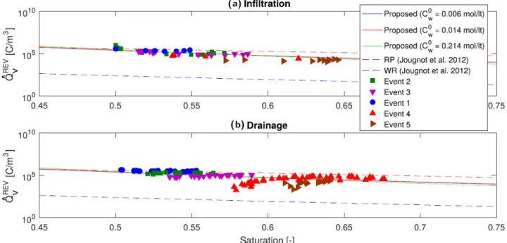
ap-proach, Jougnot et al. (2012) and later Soldi et al. (2019) tried to re-interpret the data of Doussan et al. (2002). Figure 3.14 presents the evolution of the effective excess charge with the saturation during five different rainfall event from the data. It shows that the flux-averaging approach seems to be able to reproduce the experimental data.

Figure 3.14: Effective excess charge density exctracted from the SP signal measured in Doussan et al. (2002) as a function of saturation during an (a) infiltation and (b) drainage phase of the event. Comparison of these data with the numerical WR and RP approaches of Jougnot et al. (2012) and the analytical closed form equation of Soldi et al. (2019) at three salinities (figure from Soldi et al., 2019).

Dedicated hydrogeophysical test site Jougnot et al. (2015) present a study about the use water infiltration monitoring by SP signal. We equipped the Voulund agricultural hydrogeophysical test site from the HOBE network in Denmark (Fig. 3.15a and b) with vertically distributed non-polarizable electrodes (Fig. 3.15c). This was the first work to focus on the vertical self-potential distribution prior to and during a saline tracer test. We build up a coupled hydrogeophysical modelling framework is used to simulate the SP response to precipitation and saline tracer infiltration.

The resulting model that compares favorably with electrical resistance tomography models is sub-sequently used to predict the SP response. The electrokinetic contribution (caused by water fluxes in a charged porous soil) is modeled by the flux-averaging approach from Jougnot et al. (2012) but with a

Developing hydrogeophysics for critical zone studies, importance of heterogeneities and processes at the mesoscopic scale

HAL Id: tel-02865330

https://hal.archives-ouvertes.fr/tel-02865330

Developing hydrogeophysics for critical zone studies,

importance of heterogeneities and processes at the

mesoscopic scale

Damien Jougnot

To cite this version:

DEVELOPING HYDROGEOPHYSICS FOR CRITICAL ZONE STUDIES,

IMPORTANCE OF HETEROGENEITIES AND PROCESSES AT THE

MESOSCOPIC SCALE

Damien JOUGNOT

Contents

List of Figures

Foreword

Abstract

Résumé

Chapter 1

Introduction

Chapter 2

Methods and definitions

2.1

Presentation of the considered geophysical methods

2.1.1

Electrical resistivity and induced polarization

2.1.2

Self-potential

2.1.3

Seismic and seismoelectric methods

2.2

Definition of the mesoscopic scale

2.2.1

Scales in critical zone studies

2.2.2

Identifying the mesoscopic scale

Chapter 3

Water distribution in saturated and partially

saturated porous media

3.1

Effect of preferential flow and transport on electrical

conduc-tivity

3.1.1

Development of a millifluidic geophysical set-up

3.1.2

Geolectrical monitoring of a saline tracer test at the mesoscopic scale

3.1.3

Discussion of results from the geoelectrical millifluidic experiments

3.2

Streaming current generation in partially saturated porous

media

3.2.1

Flux-averaging approach: numerical upscaling

3.2.2

Flux-averaging approach: analytical upscaling

3.2.3

Study of the effect of the pore size distribution

3.2.4

Opening for seismoelectric models

3.3

Towards a better characterization of field-scale hydrology and

hydro-ecology through the use of SP in the critical zone

3.3.1

In situ SP monitoring of rainfall events