From the complex seismogram to the pertinent information : examples from the domains of sources and structure

(1)

HAL Id: tel-00782642

https://tel.archives-ouvertes.fr/tel-00782642

Submitted on 30 Jan 2013

HAL is a multi-disciplinary open access archive for the deposit and dissemination of sci-entific research documents, whether they are pub-lished or not. The documents may come from teaching and research institutions in France or abroad, or from public or private research centers.

L’archive ouverte pluridisciplinaire HAL, est destinée au dépôt et à la diffusion de documents scientifiques de niveau recherche, publiés ou non, émanant des établissements d’enseignement et de recherche français ou étrangers, des laboratoires publics ou privés.

From the complex seismogram to the pertinent

information : examples from the domains of sources and

structure

Alessia Maggi

To cite this version:

Alessia Maggi. From the complex seismogram to the pertinent information : examples from the domains of sources and structure. Geophysics [physics.geo-ph]. Université de Strasbourg, 2010. �tel-00782642�

(2)

Université de Strasbourg

MÈMOIRE

pour obtenir l’

Habilitation à Diriger les Recherches de l’Université de Strasbourg

Spécialité : Sismologie

préparée à Ecole et Observatoire des Sciences de la Terre présentée et soutenue publiquement

par

Alessia Maggi

le 1 septembre 2010

Titre:

Du sismogramme complexe à l’information pertinente :

exemples dans le domaine des sources et des structures.

Garant de HDR: Jean-Jacques Lévêque

Jury

M. Michel Cara, Rapporteur, Président du jury

Mme. Valérie Maupin, Rapporteur

M. Guust Nolet, Rapporteur

M. Luis Rivera, Examinateur

M. Ruedi Widmer-Schnidrig, Examinateur

(3)

(4)

Résumé

Les sujets de recherche que j’ai choisi de traiter ces dix dernières années sont relativement éclectiques, couvrant des aspects relatifs tant aux sources sismiques

qu’à la structure de la Terre. Un thème fédérateur qui émerge cependant est

mon intérêt pour les nombreuses méthodes utilisées en sismologie pour extraire

l’information pertinente des sismogrammes. Dans cette thèse d’habilitation, je

parcours le fil conducteur des idées qui ont contribué à former ma pensée sur ce thème, décrivant avec plus de détails deux méthodes que j’ai développées et qui ont abouti récemment: FLEXWIN, qui permet d’identifier automatiquement dans un sismogramme complexe les fenêtres temporelles de mesure les plus appropriées dans un certain contexte, et WaveLoc, qui détecte et localise automatiquement les phénomènes sismiques à partir de formes d’ondes continues en exploitant la co-hérence de l’information sur un réseau de stations sismologiques. De tels outils, basés au départ sur l’intégration du savoir-faire “artisanal” et son automatisation, permettent en fait d’aller plus loin dans l’exploitation des sismogrammes, et sont de-venus indispensables au sismologue pour faire face au volume de données gigantesque produit par les réseaux sismologiques modernes.

(5)

Abstract

My choice of research projects over the past decade has been rather eclectic, cover-ing aspects relatcover-ing to both seismic sources and Earth structure. There is, however, a consistent theme, and that is a fascination with the large variety of methods for extracting pertinent information from seismic data. In this thesis, I give an brief, largely chronological outline of the steps and insights that have informed my cur-rent thinking on this theme, going into more detail on two methods that I have recently developed: FLEXWIN, for automatically selecting the most appropriate time-windows on complex seismograms in which to make measurements, and Wave-Loc, for automatically detecting and locating seismic phenomena from continuous waveform data by exploiting the coherence of information across a seismic network. Such tools, based on the the integration and automation of practical seismological “know-how”, allow us to exploit seismological data more completely, and are be-coming indispensable in the context of the enormous volume of data produced by modern seismic networks.

(6)

Chapter 1 Overview of past and current

research

1 Introduction

A habilitation thesis is generally regarded as an occasion to look back on one’s early years of research, and find a consistent theme that can be pursued in the future. I found this exercise particularly difficult, as my research over the past 10 years has spanned many subjects and fields, often with little apparent connection with each other. I had had the same difficulty when writing my PhD thesis in 2002, as I had undertaken three distinct subjects (earthquake depth determination, surface waveform tomography and source inversion from empirical Green’s functions). It was through discussions with Dan McKenzie during the years of my thesis, and Jean-Jacques Lévêque during my time at EOST, that I started to understand what motivated my choices of research subjects: I am fascinated by the methods of ex-tracting pertinent information from observations, by how these methods work, and how they can fail. I do not consider myself a theoretical seismologist, but more of a “data person” who, having had the good luck to learn to program very early on, is not afraid of developing software.

In this introductory chapter, I give a brief, largely chronological outline of the steps and insights that have informed my current thinking. Chapter 2 describes the first of two software packages I have developed recently, FLEXWIN, whose purpose is to automatically select, on pairs of observed and synthetic waveforms, those portions of the signal that should be used for measurement. As the FLEXWIN method is already published (Maggi et al., 2009), this chapter is relatively short, and concentrates more on the thinking behind the method than on the implementation

(9)

CHAPTER 1. OVERVIEW OF PAST AND CURRENT RESEARCH

details. Chapter 3 describes the second software package, WaveLoc, whose purpose is to detect and locate seismic phenomena using continuous data streams, and whose development is still ongoing. This rather long chapter covers the same material as a manuscript recently submitted to Geophysical Journal International, and describes the method in detail. In Chapter 4, I give a brief overview of current research efforts that are less strongly tied to the information extraction theme of this habilitation (mainly my work in Antarctica), and end with a perspective of the directions I plan to take in the near future.

2 Earthquake depths

When I started my PhD thesis in seismology in 1998, I knew next to nothing about the field, having come from a 4-years Physics program which had included only one course of Physics of the Earth containing no more than 8 hours of seismology. I started out with an apparently simple problem: inverting teleseismic waveform data for focal mechanism and earthquake depth (Maggi et al., 2000a,b, 2002). There was nothing revolutionary about the methods used in these early studies, but they were my training ground. I learned hands-on all about the insensitivity of teleseismic data to earthquake dip, about the trade-off between origin-times and earthquake depths, and about the all-important depth-phases, and how they modify the waveforms even for shallow earthquakes.

The depth distributions that came out of this early work, summarized in Fig-ure 1.1, showed that continental earthquakes occur only in the crust and not in the upper mantle, and started a heated debate in the tectonics and geodynamics community regarding the rheology of the lithosphere, debate that has continued for a decade. There are two main camps in this debate: those that favor the ‘jelly sandwich’ model of lithospheric strength (a strong upper crust, a weak lower crust, a strong mantle) and those that favor the ‘crème brulée’ model (a strong crust over a weak mantle). The former camp is headed by Dan McKenzie, and the latter by Evegeny Burov, each producing a plethora of papers (see Jackson et al., 2008; Burov, 2010, for recent contributions).

A detailed analysis of the controversy, though interesting from a scientific point of view, is outside the scope of this habilitation thesis, because I have not partici-pated in any of the work following the original re-determination of the continental earthquake depth distribution, and because the depths themselves have not since been called into question (see for example Adams et al., 2009, for confirmation of shallow continental seismicity in the Zagros mountains of Iran). The main lessons I

(10)

CHAPTER 1. OVERVIEW OF PAST AND CURRENT RESEARCH -60 -40 -20 0 0 2 4 6 Zagros

A

_-60 -40 -20 0 0 2 4 6 8 Aegean

B

-80 -40 0 0 10 20 Tibet

C

_-60 -40 -20 0 0 2 4 6 Iran Plateau

D

-60 -40 -20 0 0 2 4 6 8 10 Africa

E

_-60 -40 -20 0 0 2 4 6 8 Tien Shan

F

_-60 -40 -20 0 0 2 4 6 North India

G

Depth (km)

Figure 1.1: Histograms of earthquake focal depths determined by modeling of long-period teleseismic P (primary) and SH (secondary horizontal) seismograms (solid bars).White bar in North India (G) is depth determined from short period depth phases in Shillong Plateau by Chen and Molnar (1990). White bars in Tibet (C) are subcrustal earthquakes, but not necessarily in mantle of continental origin. Ap-proximate Moho depths determined by receiver function analyses are indicated by dashed lines. (Maggi et al., 2000a, Fig.1)

learned from this experience were: (1) not to implicitly trust parameters in earth-quake catalogs, especially not the hypocentral depth that can be incorrect by several tens of kilometers; (2) that the seismic waveform contains a wealth of information, often enough to resolve trade-offs inherent when using only selected parts of this information (i.e. phase arrival times); (3) that observations made by seismologists – even robust ones – can ignite furious debates in other communities, and that there-fore one must take care not to introduce non-robust observations into the system.

3 Surface waveform tomography

After being convinced from this early work on source parameter estimation that the key to obtaining robust results was to use the information contained in the seismic waveform, I started working in the field of surface waveform inversion and tomogra-phy, both during my PhD and during my first Postdoc at EOST, where I explored two ‘competing’ multimode surface waveform inversion techniques: the Partitioned Waveform Inversion method of Nolet (1990), and the secondary observables method of Cara and Lévêque (1987) automated by Debayle (1999). I applied the first method to the Middle East (Maggi and Priestley, 2005) and the second to the Pacific Ocean

(11)

Figure 1.2: Basic schematic of surface waveform tomography: (a),(b) Use a

wave-form inversion technique to determine a 1-D path-average upper mantle SV velocity

model. (c),(d) Retrieve the local value of SV from the set of path-average

measure-ments by tomographic inversion. (Maggi et al., 2006a,b).

Surface wave tomographies using these two methods share a common two-step framework, illustrated by Figure 1.2: the first step consists in a surface waveform inversion performed by matching mode-summation synthetic seismograms and ob-served regional surface waveforms from earthquakes with known focal parameters and depths, to produce 1-D velocity models along the great-circle propagation paths between sources and receivers; the second step consists in a tomographic inversion performed by combining the ensemble of 1-D models into a single linear system, that is then inverted by damped least squares inversion to determine the 3-D ve-locity model for the region. In this framework, the Nolet (1990) surface waveform inversion is paired with the Van der Lee and Nolet (1997) tomographic inversion, while the Cara and Lévêque (1987) surface waveform inversion is paired with the Debayle and Sambridge (2004) tomographic inversion.

Much could be written about the comparison between these two methods, which, though similar in framework, differ substantially in the implementation details. Such an exercise, though instructive for a detailed understanding of the waveform tomog-raphy problem, is once more outside the scope of this habilitation thesis, as I did not, myself, participate in the formulation of either method. I shall concentrate here on the personal considerations that I brought to two tomographic studies carried out with these methods.

In the first step of both tomographic methods, 1-D path-averaged velocity struc-tures are obtained from measurements made on pairs of observed and synthetic seis-mograms, where the synthetic seismograms are constructed by assuming a starting 1-D velocity model and an earthquake location and focal mechanism. The problems inherent in the choice of 1-D starting velocity model, and the necessity of adapting this starting model to the crustal structure between the source and station, have been well documented in the literature and will not be repeated here. Given my

(12)

CHAPTER 1. OVERVIEW OF PAST AND CURRENT RESEARCH -400 -300 -200 -100 0 3.0 3.5 4.0 4.5 5.0 -400 -300 -200 -100 0 3.0 3.5 4.0 4.5 5.0 2.5 3.0 3.5 4.0 10 20 50 100 200 2.5 3.0 3.5 4.0 10 20 50 100 200 2.5 3.0 3.5 4.0 10 20 50 100 200 2.5 3.0 3.5 4.0 10 20 50 100 200 2.5 3.0 3.5 4.0 10 20 50 100 200 2.5 3.0 3.5 4.0 10 20 50 100 200 2.5 3.0 3.5 4.0 10 20 50 100 200 2.5 3.0 3.5 4.0 10 20 50 100 200 -400 -300 -200 -100 0 3.0 3.5 4.0 4.5 5.0 -400 -300 -200 -100 0 3.0 3.5 4.0 4.5 5.0 Far Near Near Far Near Near (a) (b) Time (s) Time (s) Period (s) Period (s) Group velocity (km/s) Group velocity (km/s) Depth (km) Depth (km) Shear velocity (km/s) Shear velocity (km/s) Near Far Near Far Far Far

Figure 1.3: Sensitivity of 1-D waveform inversions to a ±50 km epicentral mislo-cation for (a) an event with epicentral distance ∼1700 km and (b) an event with epicentral distance ∼2500 km. Inversion velocity models and dispersion curves for the correct epicentral location are shown as thick black lines. If the epicentre is closer to the event than the true epicentre, then the phase arrivals will be late, and the waveform inversion will make the inversion velocity model slower to compen-sate; if the epicentre is further from the event than the true epicentre, the phase arrivals will be early, and the resulting inversion velocity model will be faster. The effects are more pronounced for shorter epicentral distances, but the quality of fit is always unchanged because the mislocation produces a timing error which does not change the amplitude and relative phase of any part of the seismogram. (Maggi and Priestley, 2005, Fig.2)

previous experience on earthquake depth and focal mechanism estimation, in which I had found numerous instances of large errors in the parameters given in earthquake catalogs, including the Engdahl catalog (Engdahl et al., 1998) and the Harvard CMT catalog, I started worrying about the influence these errors could have on the surface waveform inversion, and in particular that errors in the source parameters might be mapped into the inverted model as erroneous Earth structure.

At this time, I was working on a PWI tomography of the Middle East (Maggi and Priestley, 2005), a region for which earthquake epicenters and depths were notori-ously inaccurate due essentially to the nonexistence or inaccessibility of local seismic networks, and the poor azimuthal coverage for teleseismic observations. Lateral er-rors in epicentral location in the region could reach up to 50 km (Lohman and Simons, 2002), and I had found that earthquake depths could also be in error by up to 50 km (Maggi et al., 2000a). Lateral errors map directly into the 1-D

(13)

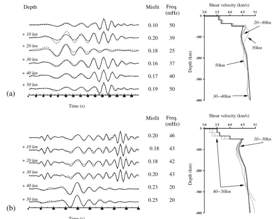
CHAPTER 1. OVERVIEW OF PAST AND CURRENT RESEARCH -400 -300 -200 -100 0 3.0 3.5 4.0 4.5 5.0 -400 -300 -200 -100 0 3.0 3.5 4.0 4.5 5.0 -400 -300 -200 -100 0 3.0 3.5 4.0 4.5 5.0 -400 -300 -200 -100 0 3.0 3.5 4.0 4.5 5.0 0.20 39 0.18 25 0.16 37 0.17 40 0.10 50 0.19 50 0.18 43 0.18 42 0.20 43 0.23 20 0.20 46 0.25 20 Misfit (mHz) Freq. (a) Time (s) + 10 km + 20 km + 30 km + 40 km + 50 km (b) Time (s) + 20 km + 30 km + 40 km + 50 km Depth (km) 20−40km 30−40km 50km 50km Depth (km) Shear velocity (km/s) 10−30km 40−50km + 10 km Shear velocity (km/s) Misfit (mHz) Freq. Depth

Figure 1.4: Sensitivity of 1-D waveform inversions to focal depths. The effects of varying focal depth for the two events in Fig 1.3: (a) focal depth 2 km (b) focal depth 9 km. Fits of final synthetic (dashed) to observed (solid) seismograms for shifts in focal depths of 10–50 km are shown on the left, and the corresponding inversion velocity models (thin lines) are shown on the right along with the velocity model for the correct depth (thick line). The misfit and maximum frequency achieved by the waveform inversion are denoted to the right of each waveform fit. (Maggi and Priestley, 2005, Fig.3)

(14)

ity models via the apparent group-velocity dispersion curves, without altering the waveform misfit (see Fig. 1.3). Depth errors lead to incorrect assumptions about the modal and frequency content of surface waves, and they can change the output 1-D velocity models significantly without necessarily having a large effect on wave-form misfit (Fig. 1.4). Errors in focal mechanisms, not unknown in the Harvard CMT catalogue for this region (Dziewonski et al., 1981; Baker et al., 1993; Maggi et al., 2000a), also affect the reliability of the 1-D models as they lead to incorrect assumptions about the phase of surface waves.

Most tomographic algorithms take into account the estimated uncertainty in the data (in our case the path-averaged shear wave velocity models) used to drive the inversion. These data errors not only regulate the relative weight given to each datum within the inversion, but also regulate how far beyond the a-priori model variance the inversion will push the final model in order to fit the data within their errors.

However, if the data are unreliable and the data errors underestimate the true uncertainties, this same behavior can lead to artifacts in the final result. I have shown above that errors in earthquake epicenter, origin time and hypocentral depth affect directly the shear wave velocity models obtained by waveform inversion, with-out any influence on the quality of the waveform fit. These source errors lead to erroneous path-averaged shear wave velocity models coupled with underestimated uncertainties, and cause artifacts in the tomographic inversion. In order to reduce these artifacts, excessive smoothing is often used, leading to loss of horizontal reso-lution and a decrease in data fit.

In my Middle East and Pacific Ocean tomographic studies, I have used two different approaches to resolve this problem. The approach for the first study was to remove the unreliable data, while that for the second study was to obtain better estimates of the true data errors.

3.1 Middle East strategy: Remove unreliable data

In my Middle East study (Maggi and Priestley, 2005), I decided to be very stringent in the data selection, and only considered data from events for which focal mecha-nisms and depths had been independently determined by body waveform modeling. This approach drastically reduced the size of my dataset, and meant I could no longer assume the effects of epicentral mislocation would average out. However, artifacts in the 3-D velocity model caused by errors in focal depth and source mechanism were minimized. In order to isolate cases of significant epicenter mislocation, I

(15)

CHAPTER 1. OVERVIEW OF PAST AND CURRENT RESEARCH 10˚ 20˚ 30˚ 40˚ 50˚ 60˚70˚ 80˚ 90˚ 0˚ 10˚ 20˚ 30˚ 40˚ 50˚ 60˚ 10˚ 20˚ 30˚ 40˚ 50˚ 60˚70˚ 80˚ 90˚ 0˚ 10˚ 20˚ 30˚ 40˚ 50˚ 60˚ -400 -300 -200 -100 0 2 3 4 5 -400 -300 -200 -100 0 2 3 4 5 Group Velocity Velocity (km/sec) Period (s) 3 4 10 20 50 100 200 3 4 10 20 50 100 200 3 4 10 20 50 100 200 3 4 10 20 50 100 200 3 4 10 20 50 100 200 3 4 10 20 50 100 200 3 4 10 20 50 100 200 3 4 10 20 50 100 200 3 4 10 20 50 100 200 3 4 10 20 50 100 200 Time (s) Shear velocity (km/s) Depth (km) 10˚ 20˚ 30˚ 40˚ 50˚ 60˚70˚ 80˚ 90˚ 0˚ 10˚ 20˚ 30˚ 40˚ 50˚ 60˚ 10˚ 20˚ 30˚ 40˚ 50˚ 60˚70˚ 80˚ 90˚ 0˚ 10˚ 20˚ 30˚ 40˚ 50˚ 60˚ -400 -300 -200 -100 0 2 3 4 5 -400 -300 -200 -100 0 2 3 4 5 Group Velocity Velocity (km/sec) Period (s) 3 4 10 20 50 100 200 3 4 10 20 50 100 200 3 4 10 20 50 100 200 3 4 10 20 50 100 200 3 4 10 20 50 100 200 3 4 10 20 50 100 200 3 4 10 20 50 100 200 3 4 10 20 50 100 200 3 4 10 20 50 100 200 Time (s) Shear velocity (km/s) Depth (km) 10˚ 20˚ 30˚ 40˚ 50˚ 60˚70˚ 80˚ 90˚ 0˚ 10˚ 20˚ 30˚ 40˚ 50˚ 60˚ 10˚ 20˚ 30˚ 40˚ 50˚ 60˚70˚ 80˚ 90˚ 0˚ 10˚ 20˚ 30˚ 40˚ 50˚ 60˚ -400 -300 -200 -100 0 2 3 4 5 -400 -300 -200 -100 0 2 3 4 5 Group Velocity Velocity (km/sec) Period (s) 3 4 10 20 50 100 200 3 4 10 20 50 100 200 3 4 10 20 50 100 200 3 4 10 20 50 100 200 3 4 10 20 50 100 200 3 4 10 20 50 100 200 3 4 10 20 50 100 200 3 4 10 20 50 100 200 3 4 10 20 50 100 200 3 4 10 20 50 100 200 Time (s) Shear velocity (km/s) Depth (km) (a) (b) (c) (d)

Figure 1.5: Examples of clustered 1-D results: (a) propagation paths; (b) wave-form fits; (c) 1-D shear wave velocity models; (d) fundamental mode group velocity dispersion curves and path integrated group velocity values from Ritzwoller and Levshin (1998) (Gray triangles) and Pasyanos et al. (2001) (black circles). (Maggi and Priestley, 2005, Fig.4)

(16)

pared final waveform inversion 1-D models and their dispersion curves for clusters of similar paths, that should therefore have produced similar 1-D velocity models (Fig. 1.5). Comparison of inversion models within each cluster enabled me to iden-tify and remove inconsistent data, but was still a ‘majority vote’ method and did not guarantee that the source parameters used in determining the remaining veloc-ity models were accurate. I therefore went one step further, and compared velocveloc-ity dispersion curves calculated from the final 1-D Earth models with the group veloc-ity dispersion previously measured by Ritzwoller and Levshin (1998) and Pasyanos et al. (2001) (Figure 1.5d), to isolate any residual erroneous 1-D models.

Of the 1100 seismograms originally chosen for analysis, the above data selection procedure accepted 550 ‘good quality’ seismograms, many of which had very sim-ilar propagation paths. The resulting uneven geographical distribution biased the tomography results towards the structure of the regions with highest path density: multiple sampling along certain paths re-enforced the structure along those paths compared with that of the crossing paths, and led to smearing artifacts in the 3-D model. I therefore thinned the paths so as to render the path coverage as uniform as possible, selecting only the highest signal-to-noise ratio seismograms from each cluster. I was left with only 303 good quality and approximately evenly-distributed paths, the inversion of which produced the tomographic model presented in detail in Maggi and Priestley (2005), and shown in Figure 1.6.

Results

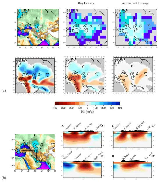
Figure 1.6a shows horizontal cross-sections through the 3-D tomographic model at 100, 150 and 250 km depth. The slices are color shaded by absolute shear wave velocity perturbation with respect to a common background model (Maggi and Priestley, 2005, Fig.6); poorly constrained areas are masked in gray. Also shown for guidance are the ray density and azimuthal coverage that are essential for a correct interpretation of the tomographic images. For example, the 250 km depth SE-NW trending slow anomaly between the Gulf of Oman and lake Balkhash in Kazakhstan passes at each end through zones of low path density, and is almost entirely contained within a region with poor azimuthal coverage, strongly suggesting that the elongated nature of the anomaly is an artifact due to smearing.

The most significant upper mantle feature of the shear wave velocity model is the low velocity zone extending beneath the Turkish–Iranian plateau. A similar image of this structure exists in the continental scale surface wave group and phase velocity maps for Asia (Ritzwoller et al., 1998; Curtis et al., 1998). Variation in shear wave velocity is caused by changes in temperature and composition as well

(17)

CHAPTER 1. OVERVIEW OF PAST AND CURRENT RESEARCH 20˚ 30˚ 40˚ 50˚ 60˚ 70˚ 80˚ 90˚ 20˚ 30˚ 40˚ 50˚ 60˚ 20˚ 30˚ 40˚ 50˚ 60˚ 70˚ 80˚ 90˚ 20˚ 30˚ 40˚ 50˚ 60˚ 20˚ 30˚ 40˚ 50˚ 60˚ 70˚ 80˚ 90˚ 20˚ 30˚ 40˚ 50˚ 60˚ 20˚ 30˚ 40˚ 50˚ 60˚ 70˚ 80˚ 90˚ 20˚ 30˚ 40˚ 50˚ 60˚ 15˚ 15˚ 20˚ 20˚ 25˚ 25˚ 30˚ 30˚ 35˚ 35˚ 40˚ 40˚ 45˚ 45˚ 50˚ 50˚ 55˚ 55˚ 60˚ 60˚ 65˚ 65˚ 70˚ 70˚ 75˚ 75˚ 80˚ 80˚ 85˚ 85˚ 90˚ 90˚ 15˚ 15˚ 20˚ 20˚ 25˚ 25˚ 30˚ 30˚ 35˚ 35˚ 40˚ 40˚ 45˚ 45˚ 50˚ 50˚ 55˚ 55˚ 60˚ 60˚ 150 km 20˚ 30˚ 40˚ 50˚ 60˚ 70˚ 80˚ 90˚ 20˚ 30˚ 40˚ 50˚ 60˚ 15˚ 15˚ 20˚ 20˚ 25˚ 25˚ 30˚ 30˚ 35˚ 35˚ 40˚ 40˚ 45˚ 45˚ 50˚ 50˚ 55˚ 55˚ 60˚ 60˚ 65˚ 65˚ 70˚ 70˚ 75˚ 75˚ 80˚ 80˚ 85˚ 85˚ 90˚ 90˚ 15˚ 15˚ 20˚ 20˚ 25˚ 25˚ 30˚ 30˚ 35˚ 35˚ 40˚ 40˚ 45˚ 45˚ 50˚ 50˚ 55˚ 55˚ 60˚ 60˚ 250 km 20˚ 30˚ 40˚ 50˚ 60˚ 70˚ 80˚ 90˚ 20˚ 30˚ 40˚ 50˚ 60˚ -400 -300 -200 -100 0 100 200 300 400 δβ (m/s) -300 -200 -100 0 -300 -200 -100 0 0 500 1000 1500 2000 2500 -200 0 -200 0 0 1000 2000 -300 -200 -100 0 -300 -200 -100 0 0 500 1000 1500 -200 0 -200 0 0 1000 20˚ 30˚ 40˚ 50˚ 60˚ 70˚ 80˚ 20˚ 30˚ 40˚ 50˚ 20˚ 30˚ 40˚ 50˚ 60˚ 70˚ 80˚ 20˚ 30˚ 40˚ 50˚ -300 -200 -100 0 -300 -200 -100 0 0 500 1000 1500 -200 0 -200 0 0 1000 -300 -200 -100 0 -300 -200 -100 0 0 500 1000 1500 2000 2500 -200 0 -200 0 0 1000 2000 15˚ 15˚ 20˚ 20˚ 25˚ 25˚ 30˚ 30˚ 35˚ 35˚ 40˚ 40˚ 45˚ 45˚ 50˚ 50˚ 55˚ 55˚ 60˚ 60˚ 65˚ 65˚ 70˚ 70˚ 75˚ 75˚ 80˚ 80˚ 85˚ 85˚ 90˚ 90˚ 15˚ 15˚ 20˚ 20˚ 25˚ 25˚ 30˚ 30˚ 35˚ 35˚ 40˚ 40˚ 45˚ 45˚ 50˚ 50˚ 55˚ 55˚ 60˚ 60˚ 100 km 20˚ 30˚ 40˚ 50˚ 60˚ 70˚ 80˚ 90˚ 20˚ 30˚ 40˚ 50˚ 60˚ (a) (b) D’ D

Turan Shield Caucasus N Zagros Arab. Shield Alborz Zagros Pers. Gulf S zagros Aegean W. Turkey E. Turkey Caspian Black Sea N./Zagros Gulf

A A’ B’ B Azimuthal Coverage Ray Density C’ D’ A A’ C C’ D B’ B C RS CT BS C CS Ar TS TSh EI M PG AS Z CI

Figure 1.6: (a) Horizontal slices through the tomographic model at 100, 150 and 250 km depth. Also shown for reference are the geographic region, and the density and azimuthal coverage images. Abbreviations on topographic map: BS – Black Sea, C – Caucasus, CT – Central Turkey, CS – Caspian Sea, Ar – Aral Sea, TS – Turan Shield, TSh – Tien Shan, Z – Zagros, CI – Central Iran, EI – Eastern Iran, RS – Red Sea, AS – Arabian Shield, PG – Persian Gulf, M – Makran. (b) Vertical cross-sections both along and across the Turkish Plateau and the Zagros mountains of southern Iran. Depths and distances along the profiles are given in km. Elevations, shown in black above the plots, are exaggerated by a factor of 10. (Maggi and Priestley, 2005, Fig.7)

(18)

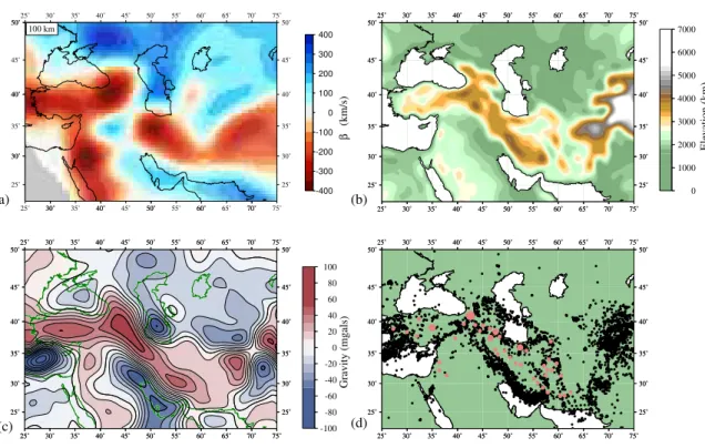
CHAPTER 1. OVERVIEW OF PAST AND CURRENT RESEARCH -100 -80 -60 -40 -20 0 20 40 60 80 100 0 1000 2000 3000 4000 5000 6000 7000 25˚ 25˚ 30˚ 30˚ 35˚ 35˚ 40˚ 40˚ 45˚ 45˚ 50˚ 50˚ 55˚ 55˚ 60˚ 60˚ 65˚ 65˚ 70˚ 70˚ 75˚ 75˚ 25˚ 25˚ 30˚ 30˚ 35˚ 35˚ 40˚ 40˚ 45˚ 45˚ 50˚ 50˚ 100 km 30˚ 40˚ 50˚ 60˚ 70˚ 30˚ 40˚ 50˚ 25˚ 25˚ 30˚ 30˚ 35˚ 35˚ 40˚ 40˚ 45˚ 45˚ 50˚ 50˚ 55˚ 55˚ 60˚ 60˚ 65˚ 65˚ 70˚ 70˚ 75˚ 75˚ 25˚ 25˚ 30˚ 30˚ 35˚ 35˚ 40˚ 40˚ 45˚ 45˚ 50˚ 50˚ 25˚ 25˚ 30˚ 30˚ 35˚ 35˚ 40˚ 40˚ 45˚ 45˚ 50˚ 50˚ 55˚ 55˚ 60˚ 60˚ 65˚ 65˚ 70˚ 70˚ 75˚ 75˚ 25˚ 25˚ 30˚ 30˚ 35˚ 35˚ 40˚ 40˚ 45˚ 45˚ 50˚ 50˚ 25˚ 25˚ 30˚ 30˚ 35˚ 35˚ 40˚ 40˚ 45˚ 45˚ 50˚ 50˚ 55˚ 55˚ 60˚ 60˚ 65˚ 65˚ 70˚ 70˚ 75˚ 75˚ 25˚ 25˚ 30˚ 30˚ 35˚ 35˚ 40˚ 40˚ 45˚ 45˚ 50˚ 50˚ 25˚ 25˚ 30˚ 30˚ 35˚ 35˚ 40˚ 40˚ 45˚ 45˚ 50˚ 50˚ 55˚ 55˚ 60˚ 60˚ 65˚ 65˚ 70˚ 70˚ 75˚ 75˚ 25˚ 25˚ 30˚ 30˚ 35˚ 35˚ 40˚ 40˚ 45˚ 45˚ 50˚ 50˚ 25˚ 25˚ 30˚ 30˚ 35˚ 35˚ 40˚ 40˚ 45˚ 45˚ 50˚ 50˚ 55˚ 55˚ 60˚ 60˚ 65˚ 65˚ 70˚ 70˚ 75˚ 75˚ 25˚ 25˚ 30˚ 30˚ 35˚ 35˚ 40˚ 40˚ 45˚ 45˚ 50˚ 50˚ 25˚ 25˚ 30˚ 30˚ 35˚ 35˚ 40˚ 40˚ 45˚ 45˚ 50˚ 50˚ 55˚ 55˚ 60˚ 60˚ 65˚ 65˚ 70˚ 70˚ 75˚ 75˚ 25˚ 25˚ 30˚ 30˚ 35˚ 35˚ 40˚ 40˚ 45˚ 45˚ 50˚ 50˚ -400 -300 -200 -100 0 100 200 300 400 (km/s) β (d) (a) (c) (b) Elevation (km) Gravity (mgals)

Figure 1.7: Comparative images of the Middle East. (a) Tomographic slice at 100 km depth; (b) regional topography low-pass filtered at 400 km; (c) free–air gravity anomalies (EGM96, Lemoine et al., 1996) low–pass filtered at 800 km; (d) regional seismicity (black circles) 1964-1998 from Engdahl et al. (1998), and Neogene–Quaternary volcanic outcrops (pink circles) (Haghipour and Aghanabati, 1989; Alavi, 1991; Choubert and Faure-Muret, 1976). (Maggi and Priestley, 2005, Fig.10)

as by the presence of volatiles and partial melt. The low shear wave velocities observed beneath the Turkish–Iranian plateau and the recent volcanism suggest that the upper mantle in this region is above the solidus temperature, a suggestion

confirmed by the poor Sn propagation found in the same region (Kadinsky-Cade

et al., 1981; Rodgers et al., 1997; Sandvol et al., 2001).

Figure 1.7 compares the pattern of low shear wave velocity observed at ∼100 km depth in the tomographic model with other geophysical and geological observations suggesting a warm, low density upper mantle beneath the Turkish–Iranian plateau. Figure 1.7c shows long wavelength (800–3500 km) free air gravity anomalies from the EGM96 dataset (Lemoine et al., 1996). There is a striking correlation between the gravity high running under the Turkish peninsula and the Zagros Mountains, and the low velocity anomaly beneath the same regions (Fig. 1.7a). Long wavelength free air gravity anomalies reflect density differences in the mantle: less dense mantle is buoyant and will tend to rise, creating an upward deflection of the surface. This

(19)

Figure 1.8: The vertical cross-section shows the model for the upper 600 km along the Zagros profile. The velocity scale saturates at ±5% of the reference background model. The dotted line shows Moho depth variations along the Zagros profile re-sulting from the inversion. Vertical and horizontal axes are depth (km) and latitude (degree) along the profile, respectively. The main tectonic units and elevation vari-ations along the Zagros profile are also shown in the top panel. (Manaman and Shomali, 2010, Fig.8)

deflection produces a larger positive gravity anomaly than the negative anomaly caused by the density deficit itself, thereby producing an overall positive anomaly and a correlation between long wavelength free air gravity anomalies and long wave-length topography. The density differences in the mantle are most likely caused by temperature differences. The distribution of volcanism across the Turkish–Iranian plateau also suggests a warm upper mantle as the source for the low shear wave velocities. Figure 1.7d shows the correlation between the locations of the low shear wave velocity zone and recent volcanism.

In Maggi and Priestley (2005) we suggest that the upper mantle low shear wave velocity zone, the high free air gravity, and the deep lithospheric source depth for the basaltic volcanism are consistent with a partial delamination of the lower litho-sphere (Pearce et al., 1990; Keskin et al., 1998), caused by an instability due to

(20)

earlier thickening of the lithospheric during the continental collision of Arabia and Eurasia. This interpretation has been called into question by later studies that pre-fer a slab break-off scenario (e.g. Paul et al., 2006), based partly on evidence for crustal-scale thrusting in the Zagros and on the shallow depths of earthquakes there (Maggi et al., 2000b). The broken-off slab has not yet been unequivocally seen in tomographic images, because of the requirement for high resolution at transition zone depths, which is difficult to obtain. Manaman and Shomali (2010) have per-formed a new PWI tomographic inversion of the Iranian region using data from the Iranian regional network and from the seismic profile across the Zagros mountains of Paul et al. (2006). They see hints of a high velocity region below Central Iran at depths of 400–600 km (Figure 1.8), but warn that the anomaly is at the limit of their resolution. The question of slab break-off for the Arabia–Eurasia collision remains to be resolved.

3.2 Pacific Ocean strategy: Estimate data errors

In my Pacific Ocean study (Maggi et al., 2006a,b), I analyzed vertical component

Rayleigh wave seismograms from all earthquakes of magnitude greater than MW 5.5

that occurred between January 1977 and April 2003, and for which the R1 portion of the surface waves propagated exclusively in the Pacific Ocean hemisphere (i.e. be-tween 120E and 300E). These earthquakes occurred mostly on the subduction zones surrounding the Pacific Plate, and to a lesser extent on the mid-ocean ridges. The vast majority of the recordings were obtained from the public IRIS (Incorporated Research Institutions for Seismology) and GEOSCOPE databases, with the addi-tion of a few thousand recordings from two years of temporary deployment of 10 seismograph stations in French Polynesia (PLUME, Barruol et al., 2002). These Polynesian records provided extra coverage in the South Pacific, allowing me to im-prove the resolution in this region compared to previous studies. The full data-set contained several hundred thousand seismograms.

The Debayle (1999) automated waveform procedure left me with a very large number of 1-D paths (56,217 ), so I decided to obtain a better estimate of the data errors by comparing multiple path averaged measurements along repeatedly sampled propagation paths. I clustered the path-averaged models geographically with a cluster radius of 200 km, and treated the shear wave models that formed each cluster as independent measurements of the average shear wave velocity profile along the common path (see Figure 1.9a for the ray density of the resulting 15,165 clusters). I took the path-averaged profile and depth-dependent measurement error

(21)

CHAPTER 1. OVERVIEW OF PAST AND CURRENT RESEARCH 1 63% (9631) 2-10 29% (4436) 11-20 21-30 31-50 >50 10 20 30 40 50 60 70 80 90 100 0.00 0.02 0.04 0.06 0.08 0.10 0 10 20 30 40 50 60 70 80 90 100 Depth = 50 km σ = 0.0475 km/s 0.00 0.02 0.04 0.06 0.08 0.10 Av. σ (km/s) 0.00 0.02 0.04 0.06 0.08 0.10 0 10 20 30 40 50 60 70 80 90 100 Depth = 100 km σ = 0.050 km/s 0.00 0.02 0.04 0.06 0.08 0.10 Av. σ (km/s)

Number of paths per cluster

0.00 0.02 0.04 0.06 0.08 0.10 0 10 20 30 40 50 60 70 80 90 100 Depth = 150 km σ = 0.057 km/s 0.00 0.02 0.04 0.06 0.08 0.10 Av. σ (km/s)

0.00 0.02 0.04 0.06 0.08 0.10 0 10 20 30 40 50 60 70 80 90 100 Depth = 200 km σ = 0.057 km/s 0.00 0.02 0.04 0.06 0.08 0.10 Av. σ (km/s)

(a) (b)

Clustered raypaths per unit area

(c)

Figure 1.9: (a) Ray density for the 15,165 clusters. The unit area is the area of a one degree cell at the equator. (b) The distribution of cluster sizes. Shading indicates the range of cluster sizes (1 path, 2–10 paths, 11–20 paths etc.); the percentage of clusters that fall in the two most populated bins are shown on the pie-chart, above the number of clusters in the bin (in brackets). (c) The average σ for clusters vs cluster size at depths of 50 to 200 km (solid lines). The average σ oscillates around a

central value ¯σ(z) indicated by the dashed lines and given within the plot. For each

depth, the range of cluster sizes for which small number statistics seem to apply (10–15) is highlighted in gray. (Maggi et al., 2006a, Fig.4)

(22)

associated with each cluster to be respectively the mean and the standard deviation on the mean of the 1D shear wave velocity models of its component paths.

Of the 15,165 clustered ray-paths, 63% contained only one path (see Fig. 1.9b), and therefore represented a single shear wave velocity measurement with no error estimate other than the a-posterior waveform fitting error. In order to use these single–path models in the tomography, they need to be assigned a reasonable data error. I averaged at each depth all the standard deviations calculated for a given cluster size. I found that this average standard deviation increased rapidly with cluster size for small clusters, before tending towards a constant value (see Fig. 1.9c). This suggested that the low value of σ for the smaller clusters was simply a low-number sampling effect, and that if there had been more data for these clusters, the standard deviation would increase to become compatible with the larger clusters. I

therefore used the flat portion of the curve to set an equivalent ¯σ for small clusters,

as shown in Fig. 1.9c, from which I calculated the corresponding data error σD(z) =

¯

σ(n)|z/√n.

The azimuthally anisotropic tomographic model obtained using this improved estimation of data errors, presented in detail in Maggi et al. (2006a) and Maggi et al. (2006b) and shown in Figures 1.10 and 1.11, enabled me to analyse the dependence of seismic velocity on the age of the oceanic lithosphere, to recover the signature of the French Polynesian plumes, and to discuss plate-motion related and plume-perturbed azimuthal anisotropy.

Dependence of seismic velocity with age

The longest wavelength isotropic feature of the tomographic model shown in

Fig-ure 1.10 is the increase in VSV with increasing ocean age, progressing from East

to West across the Pacific plate. An intuitive image of the dependence of VSV on

age can be found in the age-dependent average cross-section for the Pacific Ocean lithosphere in Figure 1.12, which was created by taking sliding window averages of the tomographic results at depths from 40 to 225 km along the isochrons of Müller

et al. (1997). VSV contours in Fig. 1.12 deepen progressively with age, approximately

following the trend predicted by Parker and Oldenburg (1973) for purely diffusive cooling. The large oscillation for ages >140 Ma coincides with a region of large

scatter in VSV, and should not be interpreted as a robust feature in the average

cooling trend.

In Maggi et al. (2006a), I compared the observed trend for VSV with ocean age

against three representative and well-known cooling models: the half-space cooling model of Parker and Oldenburg (1973) (hereafter referred to as HSC), the Parsons

(23)

CHAPTER 1. OVERVIEW OF PAST AND CURRENT RESEARCH 2% 2% 2% 2% 2% 2% -8 -7 -6 -5 -4 -3 -2-1 0 1 2 3 4 5 6 7 8 δVSV / % -8 -7 -6 -5 -4 -3 -2-1 0 1 2 3 4 5 6 7 8 δVSV / % (a) 50 km (b) 100 km (c) 150 km (d) 200 km (e) 300 km (f) 400 km

Figure 1.10: The tomographic inversion at (a) 50 km, (b) 100 km, (c) 150 km,

(d) 200 km, (e) 300 km and (f) 400 km depth. The isotropic component of VSV,

expressed as a percentage variation with respect to the model average, is indicated by the color shading. The azimuthal anisotropy results are plotted as black segments

whose direction is parallel to the fast–VSV direction, and whose length is proportional

to the amplitude of the anisotropy (the difference between maximum and minimum

VSV expressed as a percentage of the model average). The black bar at the side of

each plot is a scale bar representing 2% anisotropy. (Maggi et al., 2006b, Fig.7)

(24)

CHAPTER 1. OVERVIEW OF PAST AND CURRENT RESEARCH 100 200 300 400 100 200 300 400 0 2200 4400 6600 8800 11000 -6000 -3000 0 -6000 -3000 0 100 200 300 400 100 200 300 400 0 2200 4400 6600 8800 11000 100 200 300 400 100 200 300 400 0 2500 5000 7500 10000 12500 -6000 -3000 0 -6000 -3000 0 100 200 300 400 100 200 300 400 0 2500 5000 7500 10000 12500 100 200 300 400 100 200 300 400 0 600 1200 1800 2400 3000 -6000 -3000 0 -6000 -3000 0 100 200 300 400 100 200 300 400 0 600 1200 1800 2400 3000 100 200 300 400 100 200 300 400 0 2300 4600 6900 9200 11500 -6000 -3000 0 -6000 -3000 0 100 200 300 400 100 200 300 400 0 2300 4600 6900 9200 11500 100 200 300 400 100 200 300 400 0 1500 3000 4500 6000 7500 -6000 -3000 0 -6000 -3000 0 100 200 300 400 100 200 300 400 0 1500 3000 4500 6000 7500 100 200 300 400 100 200 300 400 0 300 600 900 1200 1500 -6000 -3000 0 -6000 -3000 0 100 200 300 400 100 200 300 400 0 300 600 900 1200 1500 -8 -7 -6 -5 -4 -3 -2 -1 0 12 3 4 5 6 7 8 δV_SV / % 20 Ma S N 80 Ma S N 40 Ma S N (a) (d) (c) (b) (h) (g) (f) 80 Ma 40 Ma 20Ma (1) EPR (3) T−K (2) Japan (e) (A) (B) (D) (C) (1) East Pacific Rise

(E) S N (2) Japan E W (3) Tonga − Kermadec E W

Figure 1.11: Selected cross-sections through our tomographic model. (a) Location of cross-sections shown in panels (b) to (d). (e) location of cross-sections shown in panels (f) to (h); the approximate boundary of the region of anomalously elevated sea-floor topography known as the South Pacific Super-Swell is indicated by a dashed line. The intersections of this boundary with the 20–80 Ma isochron profiles in panels (f)–(h) are indicated by vertical dashed lines. Green/black circles along the EPR profile in (a) and the 20–80 Ma isochron profiles in (e) correspond to the circles in panels (b), (f)–(h) and are used as distance markers. Sea-floor topography profiles from Smith and Sandwell (1997) are shown above each tomographic cross-section. Earthquakes from the Harvard CMT catalog within 200 km of the profiles are shown as small black circles. (Maggi et al., 2006a, Fig.6)

(25)

CHAPTER 1. OVERVIEW OF PAST AND CURRENT RESEARCH 50 100 150 200 250 Depth / km 20 40 60 80 100 120 140 160 Age / Myr 4.15 4.20 4.25 4.30 4.35 4.40 4.45 4.50 4.55 V_SV / km s-1 50 100 150 200 250 50 100 150 200 250 20 40 60 80 100 120 140 160 20 40 60 80 100 120 140 160

Figure 1.12: Tomographic cross-section with respect to age for the Pacific Ocean

region. This smoothed image was created by averaging VSV along the Müller et al.

(1997) isochrons, using a sliding age window of 10 Ma width and excluding areas

with no age information. Color shading represents absolute VSV. The continuous

black line indicates the position of the thermal boundary layer for the Parker and Oldenburg (1973) half-space cooling model. (Maggi et al., 2006a, Fig.10)

and Sclater (1977) plate model (hereafter referred to as PS) and the GDH1 plate model of Stein and Stein (1992). All three lithospheric cooling models fit the age-binned seismic velocities within their standard deviation, therefore the tomography itself could not formally rule out any of them. The best fit to the overall shape of

the VSV–age trend was provided by the Stein and Stein (1992) GDH1 plate model,

while HSC model and the PS thick-plate model were almost indistinguishable in terms of goodness of fit.

In order to test the robustness of any interpretation of the VSV–age curves, I

performed a synthetic tomographic experiment using a PREM + HSC input model (Maggi et al., 2006a). I computed the path averaged shear wave velocity models

along each of the 15,165 paths, and imposed the same values of σD used in the

original inversion; I then inverted this tomographic model under the same

condi-tions as the real tomographic inversion. The shape of the output VSV–age trend

was distinctly flatter than the input model between 60 and 100 Ma, and seemed to be fit better by the GHD1 model than by the HSC model. The tomographic

inversion, therefore, tended to flatten the true VSV–age trend, calling into question

my earlier conclusion that a thin plate model provided the best fit to the surface wave observations, and suggesting that a half-space cooling model or a thick plate

(26)

model was more appropriate, in accordance with most previous surface wave studies of lithospheric cooling (Forsyth, 1977; Zhang and Tanimoto, 1991; Zhang and Lay, 1999).

In a more recent, high resolution tomographic inversion of the East Pacific rise, Harmon et al. (2009) revisited the question of the conductive cooling model. They jointly inverted the data from two long-term broad-band ocean-bottom seismometer

deployments, MELT and GLIMPSE, both close to the East Pacific Rise at 17◦_{S. The}

study area covered seafloor of 0–8 Ma in age, and provided an order of magnitude better spatial resolution than that available in other studies. They found that the 16–33 s period Rayleigh wave phase velocities showed a strong square-root of seafloor age dependence, confirming that conductive cooling plays an important role in developing the seismically fast lid in the oceans.

Images of mantle plumes in French Polynesia

Panels (e)–(h) in Fig. 1.11 focus on my tomographic results for the South Pacific Super-Swell region, a shallow bathymetric anomaly (indicated by a dashed line in Fig. 1.11e) that has been postulated to be the surface expression of a large-scale mantle super-plume in the south-central Pacific Ocean (see e.g. McNutt and Fis-cher, 1987; Sichoix et al., 1998; Mégnin and Romanowicz, 2000). This region is characterized by an increased rate of volcanism compared to other oceanic regions of similar age, and has been reported as having anomalously slow shear wave veloc-ity by a number of surface wave tomographic studies (e.g. Ekström and Dziewonski, 1998; Montagner, 2002). The panels show cross-sections through the Super-Swell region and the adjacent regions of the Pacific plate, taken along the 20, 40 and 80 Ma isochrons as defined by Müller et al. (1997). The 20 Ma profile shows a localized low shear wave velocity anomaly within the Super-Swell region confined to the upper 100–150 km of the mantle. The 40 Ma profile shows two low velocity anomalies (C and D) within the Super-Swell region, associated with the approximate locations of the Marquesas and Macdonald hotspots respectively. The anomaly associated with the Macdonald hotspot (D) is continuous down to ∼420 km depth, as is the broad low velocity anomaly at the northern end of this profile, indicating a possible thermal upwelling from the transition zone. The 80 Ma profile shows a narrow low velocity anomaly (E), apparently also of thermal origin, rising from the transition zone close to the location of the Society hot-spot. It seems clear that the low velocity anomalies in the Super-Swell region, imaged with higher resolution thanks to the data from the PLUME experiment, are confined to localized structures, and are not pervasive throughout the entire area.

(27)

(a) (b)

(c) (d)

(e)

(f)

Figure 1.13: S wave velocity model in the upper mantle beneath the South Pacific. Lateral variation in S wave velocity at depths of (c) 60, (d) 100, (e) 140, and (f) 180 km. Green diamonds are active hot spots. Two-letter labels on the diamonds are the abbreviated names of the hot spots: SM, Samoa; RT, Rarotonga; SC, Society; AG, Arago; MD, Macdonald; MQ, Marquesas; PT, Pitcairn. The solid curve indicates the superswell region defined by anomalous seafloor uplift greater than 300 m. Black triangles in (a) denote temporary PLUME or BBOBS stations. Curves A-A’ and B-B’ in Figure 4c indicate locations of cross section shown in (e) and (f). (Adapted from Suetsugu et al., 2009, Fig.4 and Fig.5)

(28)

Figure 1.14: A cartoon illustrating the possible relationships between the deep su-perplume and narrower and shallower plumes beneath the South Pacific superswell. The superplume is located in the lower mantle from the core-mantle boundary to 1000 km depth. Narrow plumes beneath the hot spots may have various depth origins. The Society and Macdonald hot spots are likely deeply rooted down to the superplume head, while other hot spots may have origins in the transition zone (Pitcairn and perhaps Marquesas) or in the uppermost mantle (Arago). (Suetsugu et al., 2009, Fig.12)

In a more recent study, including data from a BBOBS (broad-band ocean-bottom seismometer) deployment in French Polynesia as well as the PLUME data, Suetsugu et al. (2009) also find low velocity anomalies of 2–3% near the Society, Macdonald, Pitcairn and Marquesas hotspots, that could represent narrow plumes in the upper mantle, confirming my observations (Figure 1.13). They also confirm that the aver-age S velocity profile beneath the South Pacific superswell is close to that of other oceanic regions whose seafloor is of a similar age, suggesting that the slow anoma-lies are localized. In the same study, Suetsugu et al. image large scale low-velocity anomalies in the superswell region, extending from the base of the mantle to a depth of 1000 km, and indicative of a superplume. They speculate that the superplume may be a hot and chemically distinct mantle dome, and that small-scale anomalies in the shape of narrow plumes may be generated from the top of the dome, as shown by the cartoon in Figure 1.14.

Anisotropy, plate motion, and mantle plumes

According to the commonly held perception of the evolution of the oceanic mantle, the ridge-normal mantle flow signature close to the mid-ocean ridges is expected

(29)

(a)

(b)

(c)

(d)

(e)

_(f)

Figure 1.15: (a) Shallow anisotropy and oceanic magnetic anomalies. The azimuthal anisotropy results for 50 km depth plotted above the magnetic anomaly traces. Magnetic anomalies are from Cande et al. (1989). (b)-(c) The correlation between

the fast VSV direction and the direction of absolute plate motion (APM) calculated

from NUVEL1 in the no-net rotation reference frame. Areas of strong correlation (anisotropy and APM directions are parallel) are shown in blue; areas of strong anti-correlation (anisotropy and APM directions are perpendicular) are shown in red; areas of weak correlation (either the directions of anisotropy and APM are at

45◦ _{to each other, or one of the two quantities is small) are shown in lighter shades of}

the two colors. (d)-(f) Synthetic test for the recovery of plume-related disturbances in azimuthal anisotropy: (d) synthetic input model with uniform 2% NW-trending anisotropy, 5 plumes of radius 200 km and 5% shear wave anomaly, and parabolic regions of rotated anisotropy; (e) output of the synthetic test; (f) correlation of the output model with respect to a ‘plate motion’ (velocity 100 mm/yr) parallel to the background anisotropy. (Adapted from Maggi et al., 2006b, Fig.8-10)

(30)

to ‘freeze’ into the fabric of the lithosphere, through lattice–preferred–orientation (LPO), as the lithosphere cools, becomes more viscous, thickens, and moves away from the ridge axis (McKenzie, 1979). The fast directions of anisotropy at litho-spheric depths are therefore expected to remain perpendicular to the magnetic lin-eations of the same age (e.g. Nishimura and Forsyth, 1989; Smith et al., 2004). Figure 1.15a shows a comparison of my azimuthal anisotropy results at 50 km depth (in the lithosphere of all but the youngest oceanic regions), with catalogued magnetic anomalies (Cande et al., 1989). The agreement is particularly good in the younger oceans, where fast azimuthal anisotropy directions are consistently perpendicular to magnetic lineations.

We observe in Figure 1.10 that the directions of anisotropy, which are hetero-geneous in the older oceans at shallow depth, tend to align themselves in longer– wavelength patterns consistent with the directions of plate motion as the depth increases and we pass from the lithosphere into the asthenosphere. Figures 1.15b,c map the correlation between azimuthal anisotropy and the directions of absolute plate motion (APM). At 150 and 200 km depth the region of good correlation (blue in the images) covers most of the Pacific Ocean. These correlation plots and the correspondence at shallow depths between azimuthal anisotropy directions and magnetic anomalies confirm the hypothesis — dating back to the earliest anisotropic studies and still in use today (Nishimura and Forsyth, 1989; Smith et al., 2004) — of stratification of the anisotropic structure in the Pacific ocean, with fossil anisotropy related to spreading directions in the lithosphere, and anisotropy conforming with current plate motion in the asthenosphere.

Also visible in Figures 1.15b,c are anomalous regions, in which the correlation be-tween azimuthal anisotropy and the direction of absolute plate motion breaks down. These anomalous regions are large (1000–3000 km), and are located in the vicinity of known hot-spots: Bowie, Juan de Fuca, Hawaii, Solomon, Samoa, Galapagos, Easter Island, Society, Marquesas, MacDonald and Louisville. This geographical correspondance suggests that the observed perturbation to the plate-motion ori-ented anisotropy may be related to mantle upwelling associated with these hot-spots. Fluid dynamical models of the interaction between an axisymmetric upwelling plume and the simple shear flow induced by a moving plate produce a flow with a roughly parabolic pattern centered over the plume, with a width several times the plume’s diameter (Kaminski and Ribe, 2002). Subsequent numerical modeling of lattice pre-ferred orientation (LPO) in this complex flow pattern using plastic deformation and dynamic re-crystallisation models predicts that the fast axes may orient themselves almost perpendicular to the parabolic flow pattern. Although the upwelling plumes

(31)

Figure 1.16: Bathymetric map of French Polynesia, showing the BBOBS (blue di-amonds), the PLUME (red circles), the IRIS/GEOSCOPE (black circles), and the LDG/CEA stations (white circles). Stars indicate locations of hotspots. Black bars represent good and gray bars fair quality measurements: The azimuth of each bar represents the fast split direction and its length the delay time between the two split arrivals. Null and anomalous splitting observations at S1 and S2 are taken as evidence for parabolic asthenospheric flow. (Barruol et al., 2009, Fig.1)

themselves are too narrow for their intrinsic anisotropic signature to be resolved, I suggested in Maggi et al. (2006b) that the large-scale perturbations of mantle flow induced by the plumes should be detectable using surface wave azimuthal anisotropy. Figures 1.15d-f show a synthetic test designed to determine the behavior of the tomographic inversion in the presence of a strong, plume-generated disturbance of the azimuthal anisotropy pattern with the geometry predicted by Kaminski and Ribe (2002). After the inversion (Figure 1.15e), the main NW-trending azimuthal anisotropy is well-recovered over most of the model, albeit with a reduction in

ampli-tude of up to a factor of two in some regions. The 90◦_{perturbation to the anisotropic}

directions present in the input model is not recovered in the synthetic inversion, how-ever the resulting anisotropic pattern is still perturbed compared to the background NW trending pattern, as is confirmed by the correlation plot (Figure 1.15f). Fur-thermore, the size and amplitude of the anti-correlation anomalies recovered in this test are similar to those found in our tomographic inversion. This test indicates

(32)

that although we do not have sufficient resolution to recover the pattern of a small or medium-scale disturbance in the anisotropy, we are able to detect its presence if the disturbance is severe enough. Recently, further evidence of parabolic astheno-spheric flow may have been found from SKS splitting measurements at ocean bottom seismometers up-stream of the Society hotspot (Barruol et al., 2009).

4 Towards full waveform tomography

The above studies using two different surface waveform tomography methods left me with the impression that, so long as the tomographic methods are well thought out and self-consistent, and the data used do not violate the assumptions and approxi-mations made by the methods, the end quality of a tomographic model is directly related to the the data themselves, and the procedures used in selecting the data, making the measurements (i.e. extracting the primary information from the data), and evaluating the true uncertainties on these measurements.

When I was starting out in tomography, discoveries were already being made about the volumetric sensitivity of certain seismic measurements (Marquering et al., 1999; Zhao et al., 2000; Dahlen et al., 2000), which opened up the possibility of calculating accurate analytic sensitivity kernels in 1D media (e.g. Dahlen and Baig, 2002; Dahlen and Zhou, 2006). These kernels were rapidly taken up by tomographers (e.g. Montelli et al., 2004; Zhou et al., 2006) to produce new 3D Earth models. The information that went into this generation of 3D Earth models was derived from measurements made with respect to synthetic seismograms (or synthetic travel-times) generated using 1-D Earth models. I had no doubts that the analytic 1D sensitivity kernels would improve the first iteration of the tomographic process, the one producing the first 3D intermediate model, but what about the following ones? Were these kernels still appropriate for the further iterations? Could one really continue the process without re-measuring, and without updating the sensitivity kernels?

At the same time, advances were also being made in computational methods for forward modeling seismic propagation in fully 3D media (Komatitsch and Vilotte, 1998; Komatitsch et al., 2002; Capdeville et al., 2003), and for calculating numerical sensitivity kernels in 3D media (e.g. Capdeville, 2005; Tromp et al., 2005; Zhao et al., 2005; Liu and Tromp, 2006, 2008), thereby opening up the possibility of ‘3D-3D’ tomography, i.e. seismic tomography based upon a 3D reference model, 3D numerical simulations of the seismic wavefield, and finite-frequency sensitivity kernels (Tromp et al., 2005; Chen et al., 2007). Measurements and sensitivity kernels could now be

(33)

made for the full seismic waveform, and updated at each iteration.

This new type of tomography would require a new type of automated data-selection strategy, in order to maximize the amount of pertinent information fed into the system at each iteration, and minimize the amount of noise. My second Postdoc, at Caltech, was dedicated to designing and implementing the data-selection strategy for the adjoint tomography method of Tromp et al. (2005). The resulting software package, FLEXWIN (distributed to the community via the Computational Infrastructure for Geodynamics, http://www.geodynamics.org) has been down-loaded by researchers all over the world, and was pivotal to producing the adjoint tomography model of Southern California (Tape et al., 2009, 2010). The FLEXWIN algorithm is described in detail by Maggi et al. (2009), a shortened version of which forms the main part of Chapter 2.

5 Coherence and earthquake location

In both the surface waveform inversion methods and the measurement methods used for adjoint tomography, the extraction of pertinent information to be tomographi-cally inverted was carried out one path at a time, by comparing pairs of observed and synthetic seismograms. The coherence of the information extracted in this manner only came into play during the tomographic inversions themselves. I had been work-ing with this kind of paradigm – make swork-ingle measurements then combine them later – for a number of years, without conscious realization. Then, during Fall AGU 2006, I attended Goran Ekstrom’s medal lecture, in which he presented his method for locating the long period energy from global earthquakes by reversing the dispersion of surface waves (Ekström, 2006). The method consists in reversing the dispersion starting from each point on a grid of possible locations in turn; the un-dispersed signals will only stack up on one of these points if an earthquake actually occurred there.

This essentially brute-force approach to the location problem was entirely based on the physical fact that information originating from a single source is necessarily coherent across a network of stations, if the waveform deformations due to source geometry and propagation are properly taken into account. I became fascinated with this concept, and rapidly developed my own version of Ekstrom’s method for the Indian Ocean, with the idea of exploiting the Southern Indian Ocean and Antarctic stations, for which I have operational responsibility, to detect long-period signals from non-standard earthquakes occurring on the mid-ocean ridges (Maggi et al., 2007). Shortly afterwards, Alberto Michelini and I started developing a method to

(34)

exploit the coherence of waveforms across the Italian national network to routinely locate local and regional earthquakes, using correlation with reference waveforms instead of de-propagation.

Development has been ongoing over the past three years, essentially as a spare time project (I have been busy with FLEXWIN and also with the International Polar Year work in Antarctica). We have presented the method at several conferences and have received enthusiastic feedback from the seismic monitoring community. The manuscript of our first WaveLoc publication, recently submitted to Geophysical Journal International, is reproduced as Chapter 3 of this habilitation thesis.

(35)

(36)

Chapter 2 FLEXWIN : automated selection of

time windows

In this chapter I shall give an outline of FLEXWIN, my open source algorithm for the automated selection of time windows on pairs of observed and synthetic seismograms.

The algorithm was designed specifically to accommodate synthetic seismograms produced from 3D wavefield simulations, which capture complex phases that do not necessarily exist in 1D simulations or traditional traveltime curves. Relying on signal processing tools and several user-tuned parameters, the algorithm is able to include these new phases and to maximize the number of measurements made on each seismic record, while avoiding seismic noise. FLEXWIN can be used in iterative tomographic inversions, in which the synthetic seismograms change from one iteration to the next, and may allow for an increasing number of windows at each model iteration. Multiple frequency bands may also be used, allowing for more detail to be included into the tomographic model at each iteration, as the higher frequency synthetics gradually start to match the data. The algorithm is sufficiently flexible to be adapted to many tomographic applications and seismological scenarios, including those based on synthetics generated from 1D models.

FLEXWIN is described in more detail in Maggi et al. (2009), and in the manual available from http://www.geodynamics.org. The algorithm was used to perform an adjoint tomography inversion of Southern California (Tape et al., 2009, 2010). Some results from this inversion will be presented at the end of this chapter.

(37)

CHAPTER 2. FLEXWIN : AUTOMATED SELECTION OF TIME WINDOWS

1 Introduction

Seismic tomography — the process of imaging the 3D structure of the Earth using seismic recordings — has been transformed by recent advances in methodology. Finite-frequency approaches are being used instead of ray-based techniques, and 3D reference models instead of 1D reference models. These transitions are motivated by a greater understanding of the volumetric sensitivity of seismic measurements (Marquering et al., 1999; Zhao et al., 2000; Dahlen et al., 2000) and by computational advances in the forward modelling of seismic wave propagation in fully 3D media (Komatitsch and Vilotte, 1998; Komatitsch et al., 2002; Capdeville et al., 2003). In the past decade we have learned to calculate analytic sensitivity kernels in 1D media (e.g. Li and Tanimoto, 1993; Dahlen and Baig, 2002; Dahlen and Zhou, 2006) and numeric sensitivity kernels in 3D media (e.g. Capdeville, 2005; Tromp et al., 2005; Zhao et al., 2005; Liu and Tromp, 2006, 2008). The analytic kernels have been taken up rapidly by tomographers, and used to produce new 3D Earth models (e.g. Montelli et al., 2004; Zhou et al., 2006). The numeric kernels have opened up the possibility of ‘3D-3D’ tomography, i.e. seismic tomography based upon a 3D reference model, 3D numerical simulations of the seismic wavefield, and finite-frequency sensitivity kernels (Tromp et al., 2005; Chen et al., 2007).

It is common practice in tomography to work only with certain subsets of the available seismic data. The choices made in selecting these subsets are inextricably linked to the assumptions made in the tomographic method. For example, ray-based traveltime tomography deals only with high-frequency body-wave arrivals, while great-circle surface-wave tomography must satisfy the path-integral approxi-mation, and only considers surface-waves that present no evidence of multipathing. In both these examples, a large proportion of the information contained within the seismograms is unused. The emerging 3D-3D tomographic methods take advantage of full wavefield simulations and numeric finite-frequency kernels, thereby reducing the data restrictions required when using approximate forward modelling and sim-plified descriptions of sensitivity. These methods seem to be the best candidates for studying regions with complex 3D structure, as they permit the use of a larger proportion of the information contained within each seismogram, including complex arrivals not predicted by 1D approximations of Earth structure. In order to ex-ploit the full power of 3D-3D tomographic methods, we require a new data selection strategy that does not exclude such complex arrivals.

As data selection strategies for tomography depend so closely on the tomographic technique, there are nearly as many such strategies as there are tomographic

(38)

CHAPTER 2. FLEXWIN : AUTOMATED SELECTION OF TIME WINDOWS

ods. Furthermore, many of these strategies have been automated in some way, as larger and larger volumes of data have become available. Body-wave studies that have moved away from using manual traveltime picks or catalog arrival times gen-erally pick windows around specific seismic phases defined by predicted traveltimes, and include automated tests on arrival time separation and/or the fit of observed to synthetic waveforms to reject inadequate data (e.g. Ritsema and van Heijst, 2002; Lawrence and Shearer, 2008). Partial automation of the VanDecar and Crosson (1990) multi-channel cross-correlation method has led to efficient methods for ob-taining highly accurate traveltime (Sigloch and Nolet, 2006; Houser et al., 2008) and even attenuation (Lawrence et al., 2006) measurements. In the surface-wave community, there has been much work done to automate methods for extracting dispersion characteristics of fundamental mode (Trampert and Woodhouse, 1995; Laske and Masters, 1996; Ekström et al., 1997; Levshin and Ritzwoller, 2001) and higher mode (Van Heijst and Woodhouse, 1997; Debayle, 1999; Yoshizawa and Ken-nett, 2002; Beucler et al., 2003; Lebedev et al., 2005; Visser et al., 2007) surface-waves. Recently, Panning and Romanowicz (2006) have described an algorithm to semi-automatically pick body and surface-wavepackets based on the predicted traveltimes of several phases.

FLEXWIN is designed for tomographic applications with 3D Earth reference models. Unlike the techniques discussed above, it is not tied to arrival time predic-tions of known phases, and, therefore, is able to accommodate complex phases due to 3D structure. One promising approach to 3D-3D tomography is based upon adjoint methods (Tarantola, 1984; Tromp et al., 2005; Liu and Tromp, 2006; Tape et al., 2007). In “adjoint tomography” the sensitivity kernels that tie variations in Earth model parameters to variations in the misfit are obtained by interaction between the wavefield used to generate the synthetic seismograms (the direct wavefield) and an adjoint wavefield that obeys the same wave equation as the direct wavefield, but with a source term which is derived from the misfit measurements. The computa-tional cost of such kernel computations for use in seismic tomography depends only on the number of events, and not on the number of receivers nor on the number of measurements. It is therefore to our advantage to make the greatest number of mea-surements on each seismogram. The adjoint kernel calculation procedure allows us to measure and use for tomographic inversion almost any part of the seismic signal. We do not need to identify specific seismic phases, as the kernel will take care of defining the relevant sensitivities. However, there is nothing in the adjoint method itself that prevents us from constructing an adjoint kernel from noise-dominated data, thereby polluting our inversion. An appropriate data selection strategy for