HAL Id: cel-00719540
https://cel.archives-ouvertes.fr/cel-00719540
Submitted on 20 Jul 2012
HAL is a multi-disciplinary open access
archive for the deposit and dissemination of sci-entific research documents, whether they are pub-lished or not. The documents may come from teaching and research institutions in France or abroad, or from public or private research centers.
L’archive ouverte pluridisciplinaire HAL, est destinée au dépôt et à la diffusion de documents scientifiques de niveau recherche, publiés ou non, émanant des établissements d’enseignement et de recherche français ou étrangers, des laboratoires publics ou privés.
Plane Topology and Dynamical Systems
Boris Kolev
To cite this version:
Boris Kolev. Plane Topology and Dynamical Systems. École thématique. Summer School ”Systèmes Dynamiques et Topologie en Petites Dimensions”, Grenoble, France, 1994, pp.35. �cel-00719540�
Plane Topology and Dynamical
Systems
Boris KOLEV
CNRS & Aix-Marseille University
Grenoble, France, June-July 1994
Summary. — These notes have been written for a Summer School, Syst`emes Dynamiques et Topologie en Petites Dimensions, which took place at the Institut Fourier, in June-July 1994. The goal was to provide simple proofs for the Jordan and Schoenflies theorems and to give a short introduction to the theory of locally connected continua and indecomposable continua, with applications in Dynamical Systems and the theory of attractors.
E-mail : [email protected]
Homepage : http://www.cmi.univ-mrs.fr/~kolev/
c
○ This work is licensed under a Creative Commons Attribution-NonCommercial-NoDerivs 3.0 Unported License.
Chapter 1
The Jordan Curve Theorem
A homeomorphic image of a closed interval [𝑎, 𝑏] (𝑎 < 𝑏) is called an arc and a homeomorphic image of a circle is called a simple closed curve or a Jordan curve. To begin with, we recall first two simple facts about the plane.
1. If 𝐹 is a closed set in R2, any component of R2− 𝐹 is open and arcwise connected. We will call these components, the complementary domains of 𝐹 .
2. If 𝐾 is a compact set in the plane R2, then R2− 𝐾 has exactly one unbounded component.
We will refer to it as the unbounded or exterior component of 𝐾.
Assertion (1) follows from the local arcwise-connectedness of R2 and (2) from the boundedness of 𝐾.
Theorem 1.1 (Jordan Curve Theorem). The complement in the plane R2 of a simple closed
curve 𝐽 consists of two components, each of which has 𝐽 as its boundary. Furthermore, if 𝐽 has complementary domains 𝑖𝑛𝑡(𝐽 ) (the bounded, or interior domain) and 𝑒𝑥𝑡(𝐽 ) (the unbounded, or exterior domain), then 𝐼𝑛𝑑(𝑥, 𝐽 ) = 0 if 𝑥 ∈ 𝑒𝑥𝑡(𝐽 ) and 𝐼𝑛𝑑(𝑥, 𝐽 ) = +1 if 𝑥 ∈ 𝑖𝑛𝑡(𝐽 ). Remark 1.2. Obviously, it follows from this statement that a simple closed curve divides the 2-sphere into exactly two domains, each of which it is the common boundary.
The proof we give here is due to Maehara [13] and uses as main ingredient the following well-known theorem of Brouwer.
Theorem 1.3 (Brouwer’s Fixed Point Theorem). Every continuous map of the closed unit disc 𝐷2 into itself has a fixed point.
Proof. We identify here the plane with the complex plane and let 𝐷2 = {𝑧 ∈ C ; |𝑧| ≤ 1} .
Suppose that 𝑓 : 𝐷2→ 𝐷2 has no fixed point. Then 𝑓 (𝑧) ̸= 𝑧 for all 𝑧 ∈ 𝐷2 and the degree1 of
each map
𝑓𝑡(𝑧) = 𝑡𝑧 − 𝑓 (𝑡𝑧), 𝑧 ∈ 𝑆1, 𝑡 ∈ [0, 1],
is well defined and all of them are equal. Since 𝑓0 is a constant map we have 𝑑(𝑓0) = 0 and
therefore 𝑑(𝑓𝑡) = 0 for all 𝑡 ∈ [0, 1]. But since |𝑧 − 𝑓 (𝑧)| is strictly positive on the compact set
𝑆1, it is bounded below by a positive constant 𝑚 and we get after an easy computation 𝑅𝑒(︀(𝑧 − 𝑓 (𝑧))¯𝑧> 𝑚
2
2 > 0,
for all 𝑧 ∈ 𝑆1 so that 𝑑(𝑓1) = 𝑑(𝐼𝑑𝑆1) = 1 which leads to a contradiction. 1
Each continuous map 𝑓 of the circle with values in C lift to a map ˜𝑓 : R → C (angle determination) which satisfies ˜𝑓 (𝜃 + 2𝜋) = ˜𝑓 (𝜃) + 2𝑑𝜋. The integer 𝑑 is called the degree of the map 𝑓 . It is easily shown to not depend on the particular lift of 𝑓 and to be a homotopy invariant.
Definition 1.4. Let 𝑋 be any metric space and 𝐴 a subspace of 𝑋. A continuous map 𝑟 : 𝑋 → 𝐴 such that 𝑟 = 𝐼𝑑 on 𝐴 is called a retraction of the space 𝑋 on 𝐴.
As a corollary of theorem 1.3 (these two statements are in fact equivalent) we have the following.
Theorem 1.5 (No-Retraction Theorem). There is no retraction of the unit disc 𝐷2 onto its boundary 𝑆1.
Proof. Suppose there exists a continuous map 𝑟 : 𝐷2 → 𝑆1 such that 𝑟(𝑧) = 𝑧 for all 𝑧 ∈ 𝑆1 and
let 𝑠 : 𝑆1 → 𝑆1 defined by 𝑠(𝑧) = −𝑧. Then the map 𝑠 ∘ 𝑟 : 𝐷2 → 𝑆1 ⊂ 𝐷2 will be a continuous
map without fixed points.
Let 𝐸 denote the square [−1, 1] × [−1, 1] and Γ = 𝐹 𝑟(𝐸) its boundary. A path 𝛾 in 𝐸 is a continuous map 𝛾 : [−1, 1] → 𝐸.
Lemma 1.6. Let 𝛾1 and 𝛾2 be two paths in 𝐸 such that 𝛾1 (resp. 𝛾2) joins the two opposite
vertical (resp. horizontal) sides of 𝐸. Then 𝛾1 and 𝛾2 have a common point.
Proof. Let 𝛾1(𝑠) = (𝑥1(𝑠), 𝑦1(𝑠)) and 𝛾2(𝑠) = (𝑥2(𝑠), 𝑦2(𝑠)) so that
𝑥1(−1) = −1, 𝑥1(1) = 1, 𝑦2(−1) = −1, 𝑦2(1) = 1.
If the two paths do not cross the function
𝑁 (𝑠, 𝑡) = max (|𝑥1(𝑠) − 𝑥2(𝑡)| , |𝑦1(𝑠) − 𝑦2(𝑡)|)
is strictly positive and the continuous map 𝑓 : 𝐸 → Γ ⊂ 𝐸 defined by 𝑓 (𝑠, 𝑡) = (︂ 𝑥2(𝑡) − 𝑥1(𝑠) 𝑁 (𝑠, 𝑡) , 𝑦1(𝑠) − 𝑦2(𝑡) 𝑁 (𝑠, 𝑡) )︂
can easily be checked to have no fixed point which contradicts the Brouwer fixed point theorem (see Exercise 1.1).
Definition 1.7. A closed set 𝐹 separates the plane R2 if R2− 𝐹 has at least two components.
Lemma 1.8. No arc 𝛼 separates the plane.
Proof. Suppose on the contrary that R2− 𝛼 is not connected. Then R2− 𝛼 has in addition to
its unbounded component 𝑈∞ at least one bounded component 𝑊 . We have 𝐹 𝑟(𝑈∞) ⊂ 𝛼 and
𝐹 𝑟(𝑊 ) ⊂ 𝛼. Let 𝑥0 ∈ 𝑊 and 𝐷 be a closed disc with centre 𝑥0 and radius 𝑅 which contains
𝑊 as well as a in its interior. By a straightforward application of the Tietze extension theorem (see Exercise 1.2) the identity map 𝐼𝑑𝛼 on 𝛼 extends continuously to a retraction 𝑟 : 𝐷 → 𝛼.
Let us define
𝑞(𝑥) =
⌉︀
𝑟(𝑥), if 𝑥 ∈ ¯𝑊 ; 𝑥, if 𝑥 ∈ 𝑊𝑐∩ 𝐷.
Then, 𝑞 : 𝐷 → 𝐷 is a continuous map whose values lie in 𝐷 − {𝑥0}. Hence, the composed map
𝑝 ∘ 𝑞 : 𝐷 → 𝐹 𝑟(𝐷) where
𝑝(𝑥) = 𝑅 𝑞(𝑥) − 𝑥0 ‖𝑞(𝑥) − 𝑥0‖
is a retraction of the disc 𝐷 onto its boundary, contradicting the no-retraction theorem (theo-rem 1.5).
Remark 1.9. For further use, note that using the same arguments we can show that no 2-cell (that is the homeomorphic image of the unit square 𝐼2) separates the plane.
Proof of Jordan’s Theorem. We will divide the proof in three steps. First we will show that 𝐽 separates the plane. Then we will prove that 𝐽 is the boundary of each of its components and finally we will prove that the complement of 𝐽 has exactly two components 𝑖𝑛𝑡(𝐽 ) and 𝑒𝑥𝑡(𝐽 ) such that 𝐼𝑛𝑑(𝑥, 𝐽 ) = 0 if 𝑥 ∈ 𝑒𝑥𝑡(𝐽 ) and 𝐼𝑛𝑑(𝑥, 𝐽 ) = ±1 if 𝑥 ∈ 𝑖𝑛𝑡(𝐽 ).
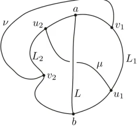
Step 1 : Since 𝐽 is compact, there exist two points 𝑎, 𝑏 in 𝐽 such that 𝑎 − 𝑏 = diam(𝐽 ). We may assume that 𝑎 = (−1, 0) and 𝑏 = (1, 0). Then the rectangular set 𝐸(−1, 1; −2, 2) contains 𝐽 , and its boundary 𝐹 meets 𝐽 in exactly two points 𝑎 and 𝑏. Let 𝑛 be the middle point of the top side of 𝐸, and 𝑠 the middle point of the bottom side. The segment 𝑛𝑠 meets 𝐽 by lemma1.6. Let 𝑙 be the 𝑦-maximal point in 𝐽 ∩ 𝑛𝑠. Points 𝑎 and 𝑏 divide 𝐽 into two arcs: we denote the one containing 𝑙 by 𝐽𝑛 and the other by 𝐽𝑠. Let 𝑚 be the 𝑦-minimal point in 𝐽𝑛∩ 𝑛𝑠 then the
segment 𝑚𝑠 meets 𝐽𝑠; otherwise, the path 𝑛𝑙 +ö𝑙𝑚 + 𝑚𝑠, (where𝑙𝑚 denotes the subarc of 𝐽ö 𝑛
with end points 𝑙 and 𝑚) could not meet 𝐽𝑠, contradicting lemma1.6. Let 𝑝 and 𝑞 denote the
𝑦-maximal point and the 𝑦-minimal point in 𝐽𝑠∩ 𝑚𝑠, respectively. Finally, let 𝑥0 be the middle
point of the segment 𝑚𝑝 (see Figure 1.1).
The choice of a homeomorphism ℎ : 𝑆1 → 𝐽 permits us to define the index of a point with respect to 𝐽 (it is well defined up to a sign). It is easy to see that 𝐼𝑛𝑑(𝑥, 𝐽 ) = 0 for any point in the unbounded complementary domain 𝑒𝑥𝑡(𝐽 ) of 𝐽 . For fixing our ideas, we suppose now that we have oriented the curve 𝐽 (resp. 𝐹 ) in such a way that we cross successively 𝑎, 𝑝 and 𝑏 (resp. 𝑎, 𝑠 and 𝑏). Let Γ𝑛 (resp. Γ𝑠) be the subarc of 𝐹 delimited by 𝑎 and 𝑏 and containing 𝑛 (resp.
𝑠). We set 𝜎𝑛= Γ𝑛− 𝐽𝑛(meaning we follow Γ𝑛, and then 𝐽𝑛 with the reversed orientation) and
𝜎𝑠= −𝐽𝑠+ Γ𝑠. Since the half line 𝑥0𝑠 does not meet 𝜎𝑛, we have 𝐼𝑛𝑑(𝑥0, 𝜎𝑛) = 0. By a similar
argument 𝐼𝑛𝑑(𝑥0, 𝜎𝑠) = 0 and since
Γ = 𝜎𝑛+ 𝐽 + 𝜎𝑠,
we have
𝐼𝑛𝑑(𝑥0, 𝐽 ) = 𝐼𝑛𝑑(𝑥0, 𝜎𝑛) + 𝐼𝑛𝑑(𝑥0, 𝐽 ) + 𝐼𝑛𝑑(𝑥0, 𝜎𝑠) = 𝐼𝑛𝑑(𝑥0, Γ) = 1.
Therefore, 𝑥0 ̸∈ 𝑒𝑥𝑡(𝐽 ) and 𝐽 separates the plane.
Step 2 : Let 𝑈 be any complementary domain of 𝐽 and 𝑥 a point in 𝑈 . Note that 𝐹 𝑟(𝑈 ) ⊂ 𝐽 . Therefore, if 𝐹 𝑟(𝑈 ) ⊂ 𝐽 , there is an arc 𝛼 which contains entirely 𝐹 𝑟(𝑈 ). Because 𝐽 separates the plane, there is a point 𝑦 ∈ R2 − 𝐽 such that 𝑥 and 𝑦 are separated by 𝐹 𝑟(𝑈 ) hence by 𝛼 which contradicts lemma 1.8. Thus 𝐹 𝑟(𝑈 ) = 𝐽 .
Step 3 : Let 𝑈 be the component of the point 𝑥0 defined in (1). Suppose that there exists
another bounded component 𝑊 (̸= 𝑈 ) of R2− 𝐽 . Clearly 𝑊 ⊂ 𝐸. We denote by 𝛽 the path 𝑛𝑙 +ö𝑙𝑚 + 𝑚𝑝 +õ𝑝𝑞 + 𝑞𝑠, whereõ𝑝𝑞 is the subarc of 𝐽𝑠, from 𝑝 to 𝑞. Hence, 𝛽 has no point of 𝑊 .
Since 𝑎 and 𝑏 are not on 𝛽, there are circular neighborhoods 𝑉𝑎and 𝑉𝑏, of 𝑎 and 𝑏, respectively,
such that each of them contains no point of 𝛽. But 𝐹 𝑟(𝑊 ) = 𝐽 , so there exist 𝑎1∈ 𝑊 ∩ 𝑉𝑎and
𝑏1 ∈ 𝑊 ∩ 𝑉𝑏. Let 𝑎ø1𝑏1 be a path in 𝑊 from 𝑎𝑙 to 𝑏1. Then the path 𝑎𝑎1+𝑎ø1𝑏1+ 𝑏𝑏𝑙 fails to
meet 𝛽. This contradicts lemma 1.6and completes the proof.
Remark 1.10. Let 𝐽 be a simple closed curve in the (oriented) plane. Then 𝐼𝑛𝑑(𝑥, 𝐽 ) = 1 for all points in 𝑖𝑛𝑡(𝐽 ) or 𝐼𝑛𝑑(𝑥, 𝐽 ) = −1 for all points in 𝑖𝑛𝑡(𝐽 ). In the first case we will say that 𝐽 is positively oriented otherwise it is negatively oriented.
From now on, a subset 𝐷 of the plane will be called a disc if it is the bounded complementary domain of a simple closed curve 𝐽 .
𝑈 being any connected open set of the plane, a cross-cut in 𝑈 is a simple arc 𝐿 ⊂ 𝑈 which intersects 𝐹 𝑟(𝑈 ) in exactly its two endpoints. If just one of the endpoints of 𝐿 meets 𝐹 𝑟(𝑈 ), then 𝐿 is called an end-cut. A point 𝑎 of 𝐹 𝑟(𝑈 ) which is the endpoint of an end-cut in 𝑈 is called accessible from 𝑈 . We will prove later that every point of a simple closed curve is accessible from both of its complementary domains.
Figure 1.1: A Jordan curve
Lemma 1.11 (𝜃-curve Lemma). Let 𝐽 be a simple closed curve in the plane. A cross-cut 𝐿 in 𝑖𝑛𝑡(𝐽 ) divides 𝑖𝑛𝑡(𝐽 ) into exactly two domains. If 𝐿1 and 𝐿2 are the subarcs of 𝐽 defined by the
endpoints 𝑎 and 𝑏 of 𝐿, these two domains are the discs 𝑖𝑛𝑡(𝐿 ∪ 𝐿1) and 𝑖𝑛𝑡(𝐿 ∪ 𝐿2).
Proof of 𝜃-curve Lemma. If 𝑋 denotes one of the sets 𝑒𝑥𝑡(𝐽 ), 𝑖𝑛𝑡(𝐿 ∪ 𝐿1) or 𝑖𝑛𝑡(𝐿 ∪ 𝐿2) then
𝐹 𝑟(𝑋) ⊂ 𝐽 ∪ 𝐿. Hence,
𝑋 ∩(︀R2− (𝐽 ∪ 𝐿)
= 𝑋 ∩ (R2− (𝐽 ∪ 𝐿)).
Therefore, 𝑋 is open and closed in R2− (𝐽 ∪ 𝐿) and is a component of R2− (𝐽 ∪ 𝐿). We are
going to show that
R2− (𝐽 ∪ 𝐿) = 𝑒𝑥𝑡(𝐽 ) ∪ 𝑖𝑛𝑡(𝐿 ∪ 𝐿1) ∪ 𝑖𝑛𝑡(𝐿 ∪ 𝐿2).
Suppose on the contrary that there exists another component 𝑈 distinct from the three above. Then 𝐹 𝑟(𝑈 ) must meet each of the three (open) arcs 𝐿∘, 𝐿∘1, 𝐿∘2. Indeed, if 𝐹 𝑟(𝑈 ∩ 𝐿∘) = ∅, then 𝐹 𝑟(𝑈 ) ⊂ 𝐽 and 𝑈 ∩ (R2− 𝐽 ) = 𝑈 ∩ (R2− 𝐽 ). Hence 𝑈 is open and closed in R2− 𝐽 and
𝑈 = 𝑖𝑛𝑡(𝐽 ) ⊃ 𝐿∘, which gives a contradiction. Similarly, if 𝐹 𝑟(𝑈 ) ∩ 𝐿∘1 = ∅, then 𝑈 is open and closed in R2− (𝐿 ∪ 𝐿2) and thus 𝑈 = 𝑒𝑥𝑡(𝐿 ∪ 𝐿2) ⊃ 𝐿∘1 which also gives a contradiction.
Therefore, we can construct a cross-cut 𝜇 in 𝑈 with endpoints 𝑢1∈ 𝐿∘1 and 𝑢2 ∈ 𝐿∘2. We can
also construct a cross-cut 𝜈 in 𝑒𝑥𝑡(𝐽 ) with endpoints 𝑣1 and 𝑣2, where 𝑣1 and 𝑣2 belong to two
non adjacent arcs among those of 𝐽 − {𝑎, 𝑢1, 𝑏, 𝑢2}. Let 𝐾 denote the simple closed curve
𝐾 = 𝜇 ∪𝑢ø1𝑣1∪ 𝜈 ∪𝑢ø2𝑣2
where 𝑢ø1𝑣1 ⊂ 𝐿∘1 and𝑢ø2𝑣2⊂ 𝐿∘2. We are therefore in the following situation (seeFigure 1.2).
1. 𝐾 ∩ 𝐿 = ∅ (since 𝜇 ⊂ 𝑈 ⊂ R2− 𝐿).
2. Each complementary domain of 𝐾 meets 𝑖𝑛𝑡(𝐽 ) and 𝑒𝑥𝑡(𝐽 ) and hence 𝐽 (since 𝜇∘ ⊂ 𝑖𝑛𝑡(𝐽 ) and 𝜈∘ ⊂ 𝑒𝑥𝑡(𝐽 )).
3. The two arcs of 𝐽 − 𝐾 are connected by 𝐿 and are therefore in one complementary domain 𝑅 of 𝐾.
4. 𝐹 𝑟(𝑅) = 𝐾 ⊃𝑢ø𝑖𝑣𝑖 (𝑖 = 1, 2).
It follows from assertions (3) and (4) that 𝐽 ⊂ 𝑅 which is a contradiction with assertion (2) (each complementary domain of 𝐾 meets 𝐽 ).
Figure 1.2: A 𝜃-curve
Theorem 1.12 (Invariance of Domain). Let 𝑈 be an open set in the plane and 𝑓 : 𝑈 → R2 be a one-to-one and continuous map. Then 𝑓 (𝑈 ) is an open set of R2.
Remark 1.13. This theorem is not to be confused with the proposition that if R2 is mapped by a homeomorphism onto itself, open sets are mapped onto open sets, which follows immediately from the definition of a homeomorphism. In this theorem, it is not assumed that the map 𝑓 is defined outside 𝑈 , nor that there exists a homeomorphism of the whole space on to itself coinciding with the given one in 𝑈 .
The proof of this theorem is an immediate application of the following Lemma. As usual 𝐷2 is the closed unit disc and 𝑆1 its boundary.
Lemma 1.14. Let 𝑓 : 𝐷2 → R2 be a continuous and one-to-one map. Then 𝑓 (𝑖𝑛𝑡(𝐷2)) =
𝑖𝑛𝑡(𝑓 (𝑆1)).
Proof. Let 𝐴 = 𝑓 (𝐷2) and 𝐽 = 𝑓 (𝑆1). Then 𝐴 is a closed 2-cell and 𝐽 is a simple closed
curve. 𝑓 (𝑖𝑛𝑡(𝐷2)) is a connected set which does not meet 𝐽 and is therefore contained in a complementary domain 𝑅 of 𝐽 . If 𝑓 (𝑖𝑛𝑡(𝐷2)) ̸= 𝑅, there are some points of R2− 𝐴 in both components of R2− 𝐽 and hence on 𝐽 since R2− 𝐴 is connected (see remark 1.9). But this is
impossible since 𝐽 ⊂ 𝐴. Therefore, 𝑓 (𝑖𝑛𝑡(𝐷2)) = 𝑅 = 𝑖𝑛𝑡(𝐽 ) (since 𝑓 (𝑖𝑛𝑡(𝐷2)) is bounded). The following corollaries of theorem1.12are straightforward and their proof will be omitted. Corollary 1.15. Let 𝑈 an open subset of the plane and 𝑓 : 𝑈 → R2 be a continuous and one-to-one map. Then 𝑓 is a homeomorphism of 𝑈 onto the open set 𝑓 (𝑈 ).
Corollary 1.16. Let 𝑓 be any homeomorphism between two plane sets 𝐴 and 𝐵. Then 𝑓 (𝑖𝑛𝑡(𝐴)) = 𝑖𝑛𝑡(𝐵). Hence, if 𝐴 and 𝐵 are closed set 𝑓 (𝐹 𝑟(𝐴)) = 𝐹 𝑟(𝐵).
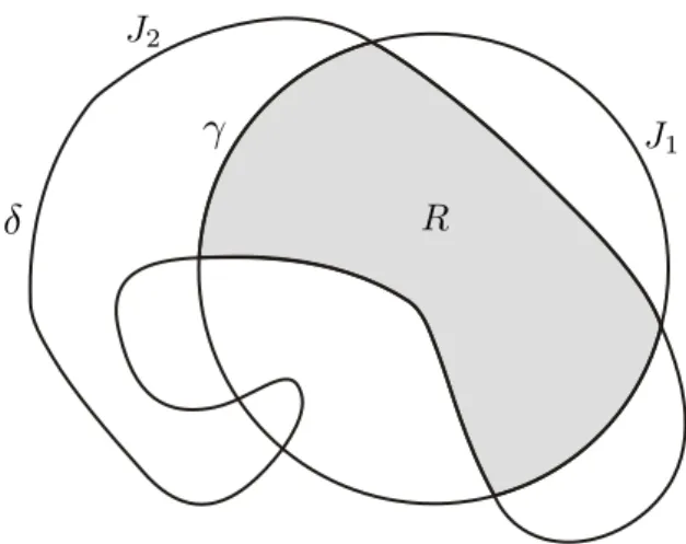
Figure 1.3: The intersection of two discs
Lemma 1.17 (Ker´ekj´art´o). Each component of the intersection of two (open) discs 𝐷1 and 𝐷2
is a disc.
Proof. If 𝐷1∩ 𝐷2 = ∅, there is nothing to prove. Otherwise, let 𝑅 be a component of 𝐷1∩ 𝐷2
and set 𝐽𝑖 = 𝐹 𝑟(𝐷𝑖) for 𝑖 = 1, 2. It is clear that 𝐹 𝑟(𝑅) ⊂ 𝐽1∪ 𝐽2. If 𝐹 𝑟(𝑅) ⊂ 𝐽𝑖 for some 𝑖,
then 𝑅 is open and closed in R2− 𝐽𝑖 hence 𝑅 = 𝐷𝑖 and the Lemma is proved. Thus, we may
assume that 𝐹 𝑟(𝑅) ̸⊂ 𝐽𝑖 for 𝑖 = 1, 2. Let 𝑥 ∈ 𝐹 𝑟(𝑅), 𝑥 ̸∈ 𝐽2. Then 𝑥 ∈ 𝐽𝑙∩ 𝐷2, and we can find
an arc 𝛾 in 𝐽1 such that 𝑥 ∈ 𝛾∘ and
𝛾∘ ⊂ 𝐷2, 𝛾 ⊂ 𝐹 𝑟(𝑅), 𝜕𝛾 ⊂ 𝐽1∩ 𝐽2.
𝐽2 ∪ 𝛾 is a 𝜃-curve and 𝑅 belongs to one of the complementary domains of R2 − 𝜃. Thus, the
endpoints of 𝛾 define an arc 𝛿 on 𝐽2 which doesn’t meet 𝑅 and such that 𝛿 ∩ 𝐹 𝑟(𝑅) = 𝜕𝛿 (see
Figure 1.3).
There is at most a countable family of such arcs 𝛾𝑛 and diam(𝛾𝑛) → 0 as 𝑛 → ∞ (see
Exercise 2.1). The corresponding arcs 𝛿∘𝑛 are pairwise disjoint (again an application of the 𝜃-curve lemma) and therefore diam(𝛿𝑛) → 0 as 𝑛 → ∞ as well. Let 𝐽 be the simple closed curve
obtained from 𝐽2 by substituting to each arc 𝛿𝑛the corresponding arc 𝛾𝑛of 𝐽1. It is then easy to
verify that 𝐹 𝑟(𝑅) ⊂ 𝐽 and therefore 𝐹 𝑟(𝑅) = 𝐽 since 𝐹 𝑟(𝑅) separates the plane but no proper closed subset of 𝐽 does. Thus 𝐹 𝑟(𝑅) is a simple closed curve and 𝑅 is a disc.
Exercises
Exercise 1.1. Let 𝐾 ̸= ∅ be a compact and convex set in the plane and 𝑓 : 𝐾 → 𝐾 a continuous map. Deduce from Brouwer’s Fixed Point Theorem that 𝑓 has at least one fixed point.
Exercise 1.2 (Tietze’s Extension Theorem). Let 𝐹 be a non empty closed set of a metric space (𝑋, 𝑑) and 𝑓 : 𝐹 → 𝐼 = [0, 1] be a continuous map. Define ¯𝑓 : 𝑋 → 𝐼 by ¯𝑓 (𝑥) = 𝑓 (𝑥), if 𝑥 ∈ 𝐹 and ¯ 𝑓 (𝑥) = sup 𝑦∈𝐹 𝑑(𝑥, 𝐹 ) 𝑑(𝑥, 𝑦)𝑓 (𝑦)
if 𝑥 ∈ 𝑋 − 𝐹 . Prove that 𝑓 is continuous. Extend the result when 𝑓 : 𝐹 → 𝐼𝑛, (𝑛 ≥ 1).
Exercise 1.3. Let 𝑈 be a connected open set in the plane. Prove that the accessible points of the boundary of 𝑈 are dense in 𝐹 𝑟(𝑈 ).
Exercise 1.4. There is no homeomorphism from the 2-sphere onto one of its proper subset. Exercise 1.5. If 𝑛 ̸= 2, R2 and R𝑛 are not homeomorphic.
Exercise 1.6. Let 𝐾 be a compact set and 𝐹 a closed set in the plane with 𝐾 ∩ 𝐹 = ∅. Let 𝑎 ∈ 𝐾 and 𝑏 ∈ 𝐹 . Show that for any 𝜀 > 0, there exists a simple closed curve 𝐽 in R2− (𝐾 ∪ 𝐹 ) which separates 𝑎 and 𝑏 and such that 𝐽 ⊂ 𝑉𝜀(𝐾).
Exercise 1.7. Deduce from Exercise 1.6 the following statements. The boundary of every bounded simply connected domain in the plane is connected. The boundary of each comple-mentary domain of a compact subset of the plane is connected.
Chapter 2
The Schoenflies Theorem
The aim of this section is to prove the famous theorem of Schoenflies which asserts that any homeomorphism of the unit circle 𝑆1 onto a simple closed curve 𝐽 can be extended to the whole plane. To do this, we now introduce an auxiliary notion which generalizes the concept of 𝜃-curve. Definition 2.1. The sum 𝐿0∪ 𝐿1 ∪ · · · ∪ 𝐿𝑛, of 𝑛 + 1 (𝑛 ≥ 1) arcs in the plane is called a
network when:
1. 𝐿0∪ 𝐿1 is a simple closed curve,
2. 𝐿𝑘∩ (𝐿0∪ 𝐿1∪ · · · ∪ 𝐿𝑘−1) consists of just the endpoints of 𝐿𝑘, for 𝑘 = 1, 2, . . . , 𝑛.
The network Γ𝑛= 𝐿0∪ 𝐿1∪ · · · ∪ 𝐿𝑛, extends Γ𝑚= 𝐿0∪ 𝐿1∪ · · · ∪ 𝐿𝑚 if 𝑚 < 𝑛 and we write
then Γ𝑚≺ Γ𝑛.
Lemma 2.2. The set R2− (𝐿0∪ 𝐿1∪ · · · ∪ 𝐿𝑛) has exactly n distinct bounded components, each of them is a disc whose boundary lies in 𝐿0∪ 𝐿1∪ · · · ∪ 𝐿𝑛.
Proof. For 𝑛 = 1 it is just Jordan’s Curve Theorem and for 𝑛 = 2, the 𝜃-curve Lemma. So, let us suppose that the Lemma is true for some 𝑛 > 2 and let 𝐷1, 𝐷2, . . . , 𝐷𝑛, be the bounded
components of 𝐷 −(𝐿0∪𝐿1∪· · ·∪𝐿𝑛). Let 𝐿𝑛+1be an arc such that 𝐿𝑛+1∩(𝐿0∪𝐿1∪· · ·∪𝐿𝑛) =
𝜕𝐿𝑛+1. Without loss of generality we can suppose that 𝐿∘𝑛+1 lies in 𝐷𝑛. By the 𝜃-curve Lemma,
we know that 𝐿𝑛+1divides 𝐷𝑛into exactly two discs 𝐷+𝑛 and 𝐷𝑛−and 𝐹 𝑟(𝐷±𝑛) ⊂ 𝐹 𝑟(𝐷𝑛)∪𝐿𝑛+1,
which proves the theorem.
Let 𝐽 = 𝐿0∪𝐿1be a simple closed curve which bounds a disc 𝐷 and Γ = 𝐿0∪𝐿1∪· · ·∪𝐿𝑛, an
extension of 𝐽 such that 𝐿𝑘 ⊂ ¯𝐷 for 𝑘 = 0, . . . , 𝑛. Then each bounded complementary domain
𝐷𝑘 (𝑘 = 1, . . . , 𝑛) of Γ is a subset of 𝐷 and ¯𝐷 =
⋃︀𝑛
𝑘=1𝐷¯𝑘. We will call the finite collection
⌋︀
¯
𝐷1, . . . , ¯𝐷𝑛
{︀
a subdivision of ¯𝐷 and we will say that Γ subdivides ¯𝐷. The number 𝑚(Γ) = max {diam(𝐷𝑘); 𝑘 = 1, . . . , 𝑛}
will be called the mesh of Γ.
Lemma 2.3. Let 𝐽 be a simple closed curve bounding a disc 𝐷 and 𝜀 > 0. Then there exists a subdivision of ¯𝐷 by a network Γ of mesh less than 𝜀.
Proof. Consider the family 𝒱 of vertical lines
𝑉𝑘= {(𝑥, 𝑦); 𝑥 = 𝑘𝜀/2} , (𝑘 ∈ Z).
Only a finite number of these lines meet 𝐷 (since 𝐷 is bounded). If 𝑉𝑘 meets 𝐷, then 𝑉𝑘∩ 𝐷 is
the union of an at most countable family of pairwise disjoint segments (𝐼𝑛𝑘) with diam(𝐼𝑛𝑘) → 0 as 𝑛 → +∞.
Let 𝛿 > 0 be such that any two points of 𝐽 with distance less than 𝛿 determine an arc on 𝐽 of diameter less than 𝜀/4 (see Exercise 2.1). Denote 𝐿2, . . . , 𝐿𝑝 those of the segments (𝐼𝑛𝑘) such
that diam(𝐼𝑛𝑘) ≥ 𝛿 and let Γ1 = 𝐽 ∪ 𝐿2∪ · · · ∪ 𝐿𝑝. Then each of the bounded complementary
domains of Γ1 is contained in the union of at most 3 adjacent vertical strips.
Indeed, suppose on the contrary that there exists a bounded complementary domain of Γ1
say 𝐷1 which meets three consecutive vertical lines 𝑉𝑘−1, 𝑉𝑘, 𝑉𝑘+1. Let 𝑎 (resp. 𝑏) a point of
𝑉𝑘−1∩ 𝐷1 (resp. 𝑉𝑘+1∩ 𝐷1). Choose a polygonal arc 𝛾 (with no vertical segments !) which joins
𝑎 and 𝑏 in 𝐷1. This arc meets 𝑉𝑘 in a finite number of points which belong to some segments
𝐼𝑛𝑘1, . . . , 𝐼𝑛𝑘𝑟 defined above. It is then easy to show by induction on 𝑟 that at least one of these segments say 𝐼𝑛𝑘1 separates the two points 𝑎 and 𝑏 in 𝐷. But 𝑑(𝑎, 𝑉𝑘) = 𝑑(𝑏, 𝑉𝑘) = 𝜀/2 so that
length(𝐼𝑛𝑘1) ≥ 𝛿, which leads to a contradiction.
Next, we do the same construction with the family ℋ of horizontal lines 𝐻𝑘 : 𝑦 = 𝑘.𝜀/2
(𝑘 ∈ Z) and we extends Γ1 into a network Γ by adding horizontal segments 𝐿𝑝+1, . . . , 𝐿𝑞 such
that each bounded complementary domain of Γ lies in the union of 3 horizontal strips. By this way we have constructed a network Γ which subdivides ¯𝐷, of mesh less than 3𝜀.
Definition 2.4. A metric space 𝑋 is uniformly locally connected provided that for any 𝜀 > 0 there exists 𝛿 > 0 so that any two points of 𝑋 with distance 𝑑(𝑥, 𝑦) < 𝛿 are contained in a connected subset of diameter less than 𝜀.
Corollary 2.5. The interior of any simple closed is uniformly locally connected.
Proof. Let 𝐽 be a simple closed curve, 𝐷 its bounded complementary domain and 𝜀 > 0 (we can suppose 2𝜀 < diam(𝐽 )). By the above Lemma, we can find a network Γ of mesh < 𝜀 with subdivides ¯𝐷. Since 2𝜀 < diam(𝐽 ) there exists 𝑖, 𝑗 such that ¯𝐷𝑖∩ ¯𝐷𝑗 = ∅ (where 𝐷1, . . . , 𝐷𝑛 are
the bounded complementary domains of Γ). Therefore, 𝛿 = min⌋︀𝑑( ¯𝐷𝑖, ¯𝐷𝑗); 𝐷¯𝑖∩ ¯𝐷𝑗 = ∅
{︀
> 0.
It is then easy to verify that two points of 𝐷 with distance less than 𝛿 can be joined in 𝐷 by an arc of diameter less than 2𝜀. Indeed, if ¯𝐷𝑖 and ¯𝐷𝑗 meet 𝐽 then ¯𝐷𝑖 and ¯𝐷𝑗 have a common arc
or there intersection is empty.
Corollary 2.6. A simple closed curve 𝐽 is accessible from both of its complementary domains. Proof. We are going to show first that every point of 𝐽 is accessible from 𝐷 = 𝑖𝑛𝑡(𝐽 ). Let 𝑎 be any point of 𝐽 and for each 𝑛 = 1, 2, . . . , let 𝛿𝑛 > 0 so that any two points in 𝐵(𝑎, 𝛿𝑛) ∩ 𝐷 can
be joined by a polygonal arc in 𝐵(𝑎, 1/𝑛) ∩ 𝐷.
For each 𝑛 choose a point 𝑥𝑛 ∈ 𝐵(𝑎, 𝛿𝑛) ∩ 𝑖𝑛𝑡(𝐽 ) and then a polygonal arc 𝛾𝑛, joining 𝑥𝑛,
and 𝑥𝑛+1 in 𝐵(𝑎, 1/𝑛) ∩ 𝐷. We define this way, a sequence of linear segments 𝑠𝑛= 𝑎𝑛𝑎𝑛+1 such
that 𝑠𝑛∩ 𝑠𝑛+1 ̸= ∅ for all 𝑛 ≥ 1 and lim(𝑎𝑛) = 𝑎. By subdividing some of the segments, we
can suppose that if 𝑠𝑖∩ 𝑠𝑗 ̸= ∅ and 𝑠𝑖 ̸= 𝑠𝑗, then 𝑠𝑖∩ 𝑠𝑗 is reduced to a common endpoint of 𝑠𝑖
and 𝑠𝑗. Hence, we define an end-cut 𝛾 connecting 𝑥1 and 𝑎 in 𝑖𝑛𝑡(𝐽 ) by the following. First, we
define 𝑘0 = max {𝑖; 𝑥1∈ 𝑠𝑖} and inductively, 𝑘𝑛+1= max {𝑖; 𝑠𝑖∩ 𝑠𝑘𝑛 ̸= ∅}. Then we set
𝛾(𝑡) = ⎧ ⎨ ⎩ 𝑠𝑘0, if 𝑡 ∈ [0, 1/2]; 𝑠𝑘𝑛, if 𝑡 ∈ [1/2 𝑛, 3/2𝑛+1]; 𝑎, t=1.
The accessibility from 𝑒𝑥𝑡(𝐽 ) follows from the following observation. A fractional linear trans-formation ℎ of the two sphere R2 ∪ {∞} which permutes a point 𝑥0 ∈ 𝑖𝑛𝑡(𝐽 ) and ∞, sends
Using similar arguments, we can show that the complement of an arc in the plane is also uniformly locally connected. In particular the endpoints of an arc are accessible from its com-plementary domain and we get the following result.
Lemma 2.7. Each arc of the plane lies in a simple closed curve.
A homeomorphism ℎ : Γ → Γ* between two networks is regular if it is possible to index the bounded complementary domains of Γ (resp. Γ*) by 𝐷1, . . . , 𝐷𝑛, (resp. 𝐷1*, . . . , 𝐷*𝑛) in such a
way that:
ℎ(𝐹 𝑟(𝐷𝑖)) = 𝐹 𝑟(𝐷*𝑖), 𝑖 = 1, . . . , 𝑛.
In that case we get also that ℎ(𝐹 𝑟(𝐷0)) = 𝐹 𝑟(𝐷*0) where 𝐷0 (resp. 𝐷0*) is the unbounded
complementary domain of Γ (resp. Γ*) (see Exercise 2.2).
Lemma 2.8. Let Γ0 and Γ1 be two networks where Γ1 extends Γ0. Then any regular
homeo-morphism ℎ0 between Γ0 and a network Γ*0 can be extended into a regular homeomorphism ℎ1
between Γ1 and an extension Γ*1 of Γ*0.
Proof. It is enough to prove the Lemma when Γ1 = Γ0 ∪ 𝐿 where 𝐿 is a simple arc. Let 𝑎, 𝑏
be the endpoints of 𝐿, hence 𝐿 ∩ Γ0 = {𝑎, 𝑏}. Without loss of generality, we can suppose that
𝐿 ⊂ ¯𝐷𝑛 so that {ℎ(𝑎), ℎ(𝑏)} ⊂ 𝐹 𝑟(𝐷*𝑛). By corollary 2.6 we can construct a cross-cut 𝐿* in
𝐷*𝑛 connecting the points ℎ(𝑎) and ℎ(𝑏). Hence we can extend ℎ on Γ1 by defining ℎ1(𝐿) = 𝐿*.
Next, we let 𝐸𝑘 = 𝐷𝑘, 𝐸𝑘* = 𝐷*𝑘for 𝑘 < 𝑛. Then we denote by 𝐸𝑛and 𝐸𝑛+1the two components
of 𝐷𝑛− 𝐿 (resp. 𝐷*𝑛− 𝐿*) indexed in such a way that ℎ1(𝐹 𝑟(𝐸𝑖)) = 𝐹 𝑟(𝐸𝑖*) for 𝑖 = 𝑛, 𝑛 + 1.
Remark 2.9. In the case where Γ1 = Γ0∪ 𝐿, we have
ℎ1(Γ1∩ ¯𝐷𝑖) ⊂ ¯𝐷*𝑖, for 𝑖 = 0, . . . , 𝑛.
This is also true by induction in the general case.
Theorem 2.10 (Schoenflies Theorem). Let 𝐽 and 𝐾 be simple closed curves. Then any home-omorphism ℎ : 𝐽 → 𝐾 can be extended to give a homehome-omorphism of 𝑖𝑛𝑡(𝐽 ) ∪ 𝐽 onto 𝑖𝑛𝑡(𝐾) ∪ 𝐾. Proof. We are going to construct inductively two sequences of networks
Γ0≺ Γ1≺ · · · Γ*0 ≺ Γ * 1≺ · · ·
and two sequences of regular homeomorphisms ℎ𝑛 : Γ𝑛 → Γ*𝑛 and ℎ*𝑛 : Γ*𝑛→ Γ𝑛 which are the
inverse of each other and such that 𝑚(Γ𝑛) < 1/𝑛, 𝑚(Γ*𝑛) < 1/𝑛 and Γ𝑛 (resp. Γ*𝑛) subdivides
¯
𝐷𝐽 = 𝑖𝑛𝑡(𝐽 ) ∪ 𝐽 (resp. ¯𝐷𝐾 = 𝑖𝑛𝑡(𝐾) ∪ 𝐾).
We set Γ0 = 𝐽 , Γ*0 = 𝐾 and ℎ0 = ℎ. Assume inductively that Γ𝑛, Γ*𝑛 and ℎ𝑛 have already
been defined so that ℎ𝑛is a regular homeomorphism of Γ𝑛onto Γ*𝑛 with inverse ℎ*𝑛and that Γ𝑛
and Γ*𝑛 subdivide ¯𝐷𝐽 and ¯𝐷𝐾 respectively.
If 𝑛 is even, we construct a subdivision Γ𝑛+1of ¯𝐷𝐾with Γ*𝑛≺ Γ*𝑛+1and 𝑚(Γ*𝑛+1) < 1/(𝑛+1).
We then extend ℎ*𝑛 into a regular homeomorphism ℎ*𝑛+1: Γ*𝑛+1 → Γ𝑛+1= ℎ*𝑛+1(Γ*𝑛+1) by virtue
of lemma 2.8.
If 𝑛 is odd we do the same construction but we extend first this time Γ𝑛 into Γ𝑛+1 with
𝑚(Γ𝑛+1) < 1/(𝑛 + 1).
Then we set Γ = ⨆︀𝑛Γ𝑛, and Γ* =
⨆︀
𝑛Γ*𝑛, and define ℎ : Γ → Γ* (resp. ℎ* : Γ* → Γ) by
ℎ(𝑥) = ℎ𝑛(𝑥) if 𝑥 ∈ Γ𝑛 (resp. ℎ*(𝑥) = ℎ𝑛(𝑥)* if 𝑥 ∈ Γ*). Then ℎ (resp. ℎ*) is uniformly
continuous. Indeed, let 𝜀 > 0 and 𝑛 > 0 be such that 1/𝑛 < 𝜀. Let 𝐷1, . . . , 𝐷𝑝𝑛 be the bounded
complementary domains of Γ𝑛 and set
𝛿𝑛= min
⌋︀
𝑑( ¯𝐷𝑖, ¯𝐷𝑗); 𝐷¯𝑖∩ ¯𝐷𝑗 = ∅
𝛿𝑛is defined for 𝑛 large enough). Then recalling that ℎ(Γ ∩ ¯𝐷𝑖) ⊂ Γ*∩ ¯𝐷𝑖*, it is straightforward
to show that for any two points of Γ with distance less than 𝛿𝑛, we have 𝑑(ℎ(𝑥), ℎ(𝑦)) < 2𝜀.
Since Γ is dense in ¯𝐷𝐽, ℎ extends uniquely to a continuous map ℎ : ¯𝐷𝐽 → ¯𝐷𝐾. Similarly ℎ*
extends to a map ℎ* : ¯𝐷𝐾 → ¯𝐷𝐽 and we get ℎ ∘ ℎ* = 𝐼𝑑 and ℎ*∘ ℎ = 𝐼𝑑 which completes the
proof.
Corollary 2.11. Let 𝐽 and 𝐾 be simple closed curves. Then any homeomorphism ℎ : 𝐽 → 𝐾 can be extended into a homeomorphism ℎ : R2→ R2 which is the identity outside a compact set.
Proof. We can suppose that 𝐾 = 𝑆1 and that the origin 𝑂 belongs to 𝑖𝑛𝑡(𝐽 ). Then, we choose a circle 𝐶 such that 𝐽 and 𝑆1 are contained in 𝑖𝑛𝑡(𝐶).
The half line 𝑂𝑥− meets 𝐽 a last time at a point a before meeting 𝐶 at a point 𝑎′ and the half line 𝑂𝑥+ meets 𝐽 a last time at a point 𝑏 before meeting 𝐶 at a point 𝑏′. Let 𝐿0 and 𝐿1 be
the two arcs of 𝐽 defined by 𝑎 and 𝑏 and 𝐿*𝑖 = ℎ−1(𝐿𝑖) (𝑖 = 0, 1).
We choose two disjoint arcs 𝐿*𝑎 and 𝐿*𝑏 in the annulus defined by 𝑆𝑙 and 𝐶 so that 𝐿*𝑎 joins ℎ−1(𝑎) and 𝑎′ and 𝐿*𝑏 joins ℎ−1(𝑏) and 𝑏′ (see Figure 2.1). Then, we extend ℎ by ℎ(𝐿*𝑎) = 𝑎𝑎′,
ℎ(𝐿*𝑏) = 𝑏𝑏′ and by the identity on 𝐶. This extension of ℎ is a regular homeomorphism between the two networks
𝐶 ∪ 𝐿*𝑎∪ 𝐿*0∪ 𝐿*𝑏 ∪ 𝐿*1, and
𝐶 ∪ 𝑎𝑎′∪ 𝐿0∪ 𝑏𝑏′∪ 𝐿1.
Now by Schoenflies theorem, it can be extended into a homeomorphism of the closed disc bounded by 𝐶. Since ℎ = 𝐼𝑑 on 𝐶, we can then extend ℎ to the whole plane by letting ℎ = 𝐼𝑑 on 𝑒𝑥𝑡(𝐶).
J
Figure 2.1:
Remark 2.12. In fact we have also proved that if 𝐽 and 𝐾 are two simple closed curve such that 𝐽 ⊂ 𝑖𝑛𝑡(𝐾), there exists a homeomorphism of the plane (with compact support) sending 𝑖𝑛𝑡(𝐾) ∩ 𝑒𝑥𝑡(𝐽 ) onto the annulus
𝐴 =⌋︀(𝑥, 𝑦) ∈ R2; 1 ≤ 𝑥2+ 𝑦2 ≤ 2{︀.
Let ℎ : R → R2 be a proper embedding and 𝐿 = ℎ(R). The closure of 𝐿 in the extended plane R2∪ {∞} is a simple closed curve and therefore:
Corollary 2.13. Any proper embedding ℎ : R → R2 can be extended into a homeomorphism of
the whole plane.
Since any arc of the plane belongs to a simple closed curve (lemma 2.7), we also get: Corollary 2.14. Any homeomorphism ℎ : [0, 1] → 𝛼 ⊂ R2 can be extended to a homeomorphism of the whole plane (with compact support).
We suppose now that we have oriented the plane. Let 𝑓 : 𝑈 → 𝑉 be a homeomorphism between two open sets of the plane. Choose a point 𝑎 ∈ 𝑈 and 𝜀 > 0 with 𝐵(𝑎, 𝜀) ∈ 𝑈 and let 𝐽 be any simple closed curve with 𝑎 ∈ 𝑖𝑛𝑡(𝐽 ) and 𝐽 ⊂ 𝐵(𝑎, 𝜀).
From Schoenflies theorem we know that ¯𝐷𝐽 = 𝑖𝑛𝑡(𝐽 ) ∪ 𝐽 is a 2-cell and from theorem 1.12
we know that the inner domain of 𝐽 is mapped by 𝑓 onto the inner domain of 𝑓 (𝐽 ). Hence there exists 𝑒 ∈ {−1, +1} such that
Ind(𝑓 (𝑎), 𝑓 (𝐽 )) = 𝑒 Ind(𝑎, 𝐽 ).
The number 𝑒 is independent of the choice of 𝐽 since two simple closed curves, 𝐽 and both containing 𝑎 in their inner domain and both contained in 𝐵(𝑎, 𝜀) are isotopic in 𝑈 − {𝑎}. The number 𝑒 = 𝑑(𝑎, 𝑓 ) is the degree of 𝑓 at 𝑎. Since 𝑎 ↦→ 𝑑(𝑎, 𝑓 ) is locally constant it is constant on any domain.
Definition 2.15. We say that a homeomorphism 𝑓 : 𝑈 → 𝑉 between two domains is orientation-preserving or orientation-reversing according to 𝑑(𝑓 ) is +1 or −1.
This definition extends easily when 𝑈 and 𝑉 are two oriented connected 2-dimensional topological manifolds or when 𝑓 is an embedding.
Exercises
Exercise 2.1. Let 𝐽 be a simple closed curve. Prove that for all 𝜀 > 0, there exists 𝛿 > 0 such that if 𝑥 and 𝑦 are two distinct points such that 𝑑(𝑥, 𝑦) < 𝛿 then at least one of the two arcs of 𝐽 delimited by 𝑥 and 𝑦 has diameter < 𝜀. Give and prove a similar statement for a simple arc. Exercise 2.2. Let ℎ : Γ → Γ*be a regular homeomorphism and 𝐷0(resp. 𝐷0*) be the unbounded
component of Γ (resp. Γ*). Show that 𝑓 (𝐹 𝑟(𝐷0)) = 𝐹 𝑟(𝐷*0).
Exercise 2.3. Let 𝑓 : 𝑈 → 𝑉 be a 𝐶𝑙 diffeomorphism between two open set in the plane. Show that 𝑑(𝑎, 𝑓 ) = +1 if det[𝑓′(𝑎)] > 0 and 𝑑(𝑎, 𝑓 ) = −1 if det[𝑓′(𝑎)] < 0.
Chapter 3
Locally Connected Continua
Definition 3.1. A continuum is a nonempty, compact, connected metric space. It is non degenerate provided it contains more than one point.
A point 𝑥 of a continuum 𝑋 is a cut point of 𝑋 if 𝑋 − {𝑥} is not connected. If 𝑌 is any subset of 𝑋, the notation 𝑌 = 𝑈 |𝑉 means that 𝑌 = 𝑈 ∪ 𝑉 is a partition of 𝑌 into two nonempty sets both open and closed in 𝑌 . The proof of the following statement is straightforward and will be omitted.
Lemma 3.2. If 𝑥 is a cut point of a continuum 𝑋 and 𝑋 − {𝑥} = 𝑈 |𝑉 , then ¯𝑈 = 𝑈 ∪ 𝑥, ¯
𝑉 = 𝑉 ∪ 𝑥 and ¯𝑈 , ¯𝑉 are both sub-continua of 𝑋.
Lemma 3.3. Let 𝑋 be a nondegenerate continuum. If 𝑋 has a cut point 𝑥 and 𝑋 − {𝑥} = 𝑈 |𝑉 , then both of 𝑈 and 𝑉 contain a non-cut point of 𝑋. In particular every nondegenerate continuum has at least two non-cut points.
Proof. Suppose that 𝑈 contains only cut points of 𝑋 and choose a countable dense set in 𝑋, 𝐸 = {𝑥𝑛; 𝑛 ∈ N} .
Let 𝑛1 be the first index 𝑛 for which 𝑥𝑛∈ 𝑈 . Since 𝑥𝑛1 is a cut point, we can find two open sets
𝑈1 and 𝑉1 such that
𝑋 − {𝑥𝑛1} = 𝑈1∪ 𝑉1, 𝑥 ∈ 𝑉1
so that ¯𝑈1 = 𝑈1∪ {𝑥𝑛1} ⊂ 𝑈 = 𝑈0.
Assume inductively that 𝑥𝑛𝑘, 𝑈𝑘 and 𝑉𝑘 have already been defined with ¯𝑈𝑘 ⊂ 𝑈𝑘−1. Then
we let 𝑛𝑘+1 be the smallest integer 𝑛 so that 𝑥𝑛 ∈ 𝑈𝑘 and we choose two open sets 𝑈𝑘+1 and
𝑉𝑘+1 such that 𝑋 −
⌋︀
𝑥𝑛𝑘+1
{︀
= 𝑈𝑘+1|𝑉𝑘+1 with 𝑥𝑘 ∈ 𝑉𝑘+1 and hence ¯𝑈𝑘+1 ⊂ 𝑈𝑘.
Then we set 𝐾 = ⋂︁ 𝑛≥0 ¯ 𝑈𝑛= ⋂︁ 𝑛≥0 𝑈𝑛
and choose a point 𝑥∞ ∈ 𝐾. We can find two open sets 𝑈∞ and 𝑉∞ such that 𝑋 − {𝑥∞} =
𝑈∞|𝑉∞. Since 𝑥∞̸= 𝑥𝑛𝑘 for all 𝑘 ≥ 1, there is an infinity of values of 𝑘 for which, say, 𝑥𝑛𝑘 ∈ 𝑉∞
and so ¯𝑈∞ = 𝑈∞∪ {𝑥∞} ⊂ 𝑈𝑘. Hence ¯𝑈∞ ⊂ 𝐾. But then, since 𝑈∞ is a nonempty open set,
there must be a point 𝑥𝑚 ∈ 𝑈∞ which leads to a contradiction since 𝐾 has been constructed so
that it contains no point of 𝐸.
Theorem 3.4. A continuum 𝑋 is an arc if it has only two non-cut points
Proof. Denote by 𝑎 and 𝑏 the two non-cut points of 𝑋. It follows from lemma 3.3 that if 𝑥 ∈ 𝑋 − {𝑎, 𝑏}, then we can find two open sets 𝐴𝑥 ∋ 𝑎 and 𝐵𝑥 ∋ 𝑏 with 𝑋 − {𝑥} = 𝐴𝑥|𝐵𝑥. It is
then easy to check that for any two such decompositions 𝑋 − {𝑥} = 𝐴𝑥|𝐵𝑥and 𝑋 − {𝑦} = 𝐴𝑦|𝐵𝑦
∙ 𝑦 ∈ 𝐵𝑥 ⇒ ¯𝐴𝑥⊂ 𝐴𝑦 and ¯𝐵𝑦 ⊂ 𝐵𝑥,
∙ 𝑦 ∈ 𝐴𝑥 ⇒ ¯𝐴𝑦 ⊂ 𝐴𝑥 and ¯𝐵𝑥⊂ 𝐵𝑦.
From this it follows first that the sets ¯𝐴𝑥 and ¯𝐵𝑥are uniquely defined for all 𝑥 ∈ 𝑋 − {𝑎, 𝑏} and
that we define a simple ordering on 𝑋 if we set: 1. 𝑥 ≺ 𝑏, for all 𝑥 ∈ 𝑋 − {𝑏},
2. 𝑥 ≺ 𝑎, for all 𝑥 ∈ 𝑋 − {𝑎},
3. 𝑥 ≺ 𝑦, if and only if 𝑦 ∈ 𝐵𝑥, for all 𝑥, 𝑦 ∈ 𝑋 − {𝑎, 𝑏}.
Moreover, if 𝑥 and 𝑦 are any two points of 𝑋 such that 𝑥 ≺ 𝑦, then there exists 𝑧 ∈ 𝑋 so that 𝑥 ≺ 𝑧 ≺ 𝑦.
Choose a countable dense set {𝑥𝑙, 𝑥2, . . . } ⊂ 𝑋. An order preserving homeomorphism ℎ :
[0, 1] → 𝑋 can now be constructed inductively as follows. We set ℎ(0) = 𝑎 and ℎ(1) = 𝑏. For each dyadic fraction 0 < 𝑚/2𝑘 < 1 with 𝑚 odd, let us assume inductively that ℎ((𝑚 − 1)/2𝑘) andℎ((𝑚 + 1)/2𝑘) have already been defined. Then choose the smallest index 𝑗 so that
ℎ(𝑚 − 1
2𝑘 ) ≺ 𝑥𝑗 ≺ ℎ(
𝑚 + 1 2𝑘 )
and set ℎ(𝑚/2𝑘) = 𝑥𝑗. It is not difficult to show that the ℎ constructed in this way on dyadic
fractions extends uniquely to an order preserving map from [0, 1] to 𝑋, which is necessarily a homeomorphism.
Corollary 3.5. A nondegenerate continuum whose connection is destroyed by the removal of two arbitrary points is a simple closed curve.
Proof. Let 𝑥 and 𝑦 be two non-cut points of 𝑋 and choose two open sets 𝑈 and 𝑉 so that 𝑋 − {𝑥, 𝑦} = 𝑈 |𝑉 . First, it is straightforward to check that ¯𝑈 = 𝑈 ∪ {𝑥, 𝑦}, ¯𝑉 = 𝑉 ∪ {𝑥, 𝑦} that there are both connected. We are going to show that ¯𝑈 and ¯𝑉 are both arcs with endpoints 𝑥, 𝑦 and hence 𝑋 = ¯𝑈 ∪ ¯𝑉 is a simple closed curve.
At least one of the two continuum 𝑈 and 𝑉 is an arc with endpoints 𝑥, 𝑦. If not, we can find 𝑧 ∈ ¯𝑈 − {𝑥, 𝑦} and 𝑡 ∈ ¯𝑉 − {𝑥, 𝑦} which are non-cut points of ¯𝑈 and ¯𝑉 respectively. Hence
𝑋 − {𝑧, 𝑡} = ( ¯𝑈 − {𝑧}) ∪ ( ¯𝑉 − {𝑡}) is connected which is a contradiction.
In fact both of them are arcs with endpoints 𝑥, 𝑦. If not, suppose for example that ¯𝑈 is not an arc. Then we can find 𝑧 ∈ 𝑈 so that ¯𝑈 − {𝑧} is connected. Hence, since ¯𝑉 is an arc, we can find 𝑡 ∈ 𝑉 such that ¯𝑉 − {𝑡} = 𝑅 ∪ 𝑆 where 𝑅 and 𝑆 are two connected sets with 𝑥 ∈ 𝑅 and 𝑦 ∈ 𝑆. Therefore
𝑋 − {𝑧, 𝑡} = ( ¯𝑈 − {𝑧}) ∪ 𝑅 ∪ 𝑆 is connected, contrary to the assumption.
Theorem 3.6 (Converse of Jordan’s Curve Theorem). Let 𝑋 be a plane continuum which has two distinct complementary domains 𝑅0, 𝑅1 from which it is at every point accessible. Then 𝑋
is a simple closed curve.
Proof. In view of what we have just shown, it is enough to prove that the connection of 𝑋 is destroyed by the removal of two arbitrary points. Let 𝑥 and 𝑦 be two distinct points of 𝑋. Since both 𝑥 and 𝑦 are accessible from 𝑅0 and 𝑅1, it is possible to find a cross-cut 𝛼𝑖 with endpoints
𝑥, 𝑦 in 𝑅𝑖 for 𝑖 = 0, 1. Hence 𝐽 = 𝛼0∪ 𝛼1 is a simple closed curve. But 𝑖𝑛𝑡(𝐽 ), like 𝑒𝑥𝑡(𝐽 ),
meets 𝑅0 and 𝑅1 and thus also 𝑋 = 𝐹 𝑟(𝑅0) = 𝐹 𝑟(𝑅1). Therefore
𝑋 − {𝑥, 𝑦} = (𝑖𝑛𝑡(𝐽 ) ∩ 𝑋) ∪ (𝑒𝑥𝑡(𝐽 ) ∩ 𝑋) is not connected.
Let 𝑋 be a metric space. We recall that 𝑋 is locally connected at a point 𝑥 ∈ 𝑋 if there exist arbitrary small connected neighborhoods of 𝑥 in 𝑋. We leave as an exercise the proof of the following.
Lemma 3.7. The following conditions are equivalent. 1. 𝑋 is locally connected at every point 𝑥 ∈ 𝑋,
2. Every point of 𝑋 possesses arbitrary small open connected neighborhoods, 3. Every connected component of an open subset of 𝑋 is itself open in 𝑋.
A space is arcwise connected if any two given points can be joined by an arc.
Theorem 3.8. In a compact and locally connected space 𝑋, each connected open set is arcwise connected.
In other words, two points of a connected open set can be joined by an arc lying entirely in 𝑈 . The desired arc will be obtained as an intersection of a sequence 𝐾1 ⊃ 𝐾2 ⊃ · · · of “thinner
and thinner” sub-continua of 𝑈 . To do this carefully, let us first define an auxiliary notion. A simple chain is a finite sequence 𝒞 = (𝐶𝑙, . . . , 𝐶𝑛) of nonempty sets such that every
two adjacent terms of the sequence intersect but no two non-adjacent terms do so. The sets 𝐶𝑙, . . . , 𝐶𝑛 are called the links of 𝒞, and if 𝑎 ∈ 𝐶1 and 𝑏 ∈ 𝐶𝑛, then 𝒞 is said to be a chain from
𝑎 to 𝑏.
If 𝒟𝑙 and 𝒟2 are simple chains such that the concatenation of the sequence 𝒟𝑙 followed by
the sequence 𝒟2 is a simple chain 𝒟, we will write 𝒟 = 𝒟𝑙+ 𝒟2. Note that if 𝒟 = 𝒟𝑙+ · · · + 𝒟𝑘,
then for 𝑖 < 𝑗 each link of 𝒟𝑖 precedes each link of 𝒟𝑗 in 𝒟.
Proof of theorem 3.8. Let 𝑈 be a nonempty connected open subset of 𝑋 and 𝑎, 𝑏 ∈ 𝑈 , 𝑎 ̸= 𝑏. It is easy to obtain a sequence 𝒞1, 𝒞2, . . . of simple chains from 𝑎 to 𝑏, 𝒞𝑛= (𝐶𝑛𝑙, . . . , 𝐶𝑛𝑘𝑛), such
that for each 𝑛:
1. every link of 𝒞𝑛 is a connected open subset of 𝑈 of diameter less than 1/𝑛,
2. the closure of each link of 𝒞𝑛+1 is a subset of some link of 𝒞𝑛,
3. there exists chains 𝒟𝑛𝑙, . . . , 𝒟𝑛𝑘𝑛 such that 𝒞𝑛+1 = 𝒟𝑛𝑙 + · · · + 𝒟𝑛𝑘𝑛 and such that each link of 𝒟𝑖𝑛 is a subset of 𝒞𝑖𝑛 for 𝑖 = 1, . . . , 𝑘𝑛.
For each 𝑛, let 𝐾𝑛 denote the union of the closures of all the links of 𝒞𝑛and let
𝐾 =
∞
⋂︁
𝑛=1
𝐾𝑛.
It is clear that 𝐾 is a continuum lying in 𝑈 and containing 𝑎 and 𝑏. To prove that 𝐾 is an arc it is sufficient to show that each point of 𝐾 − {𝑎, 𝑏} is a cut point of 𝐾. To this end, suppose 𝑝 ∈ 𝐾 − {𝑎, 𝑏} and for each 𝑛 let 𝐴𝑛 (respectively 𝐵𝑛) be the set of all 𝑥 ∈ 𝐾 such that every
link of 𝒞𝑛 containing 𝑥 precedes (follows) every link of 𝒞𝑛 containing 𝑝. Then
𝐴 = ∞ ⋃︁ 𝑛=1 𝐴𝑛 and 𝐵 = ∞ ⋃︁ 𝑛=1 𝐵𝑛
are two open sets of 𝐾 such that 𝑎 ∈ 𝐴, 𝑏 ∈ 𝐵, 𝐴 ∩ 𝐵 = ∅ (since 𝐴1 ⊂ 𝐴2 ⊂ . . . and
𝐵1⊂ 𝐵2 ⊂ . . . ) and 𝐾 − {𝑝} = 𝐴 ∪ 𝐵.
Lemma 3.9. Any continuous image of a compact locally connected space is compact and locally connected.
Proof. let 𝑈 be an open set of 𝑌 = 𝑓 (𝑋) and 𝐶 be a connected component of 𝑈 . We have to show that 𝐶 is itself open in 𝑌 . Let (𝑁𝛼) be those components of 𝑓−𝑙(𝑈 ) which meets 𝑓−1(𝐶).
Then 𝑓−1(𝐶) =⋃︀𝛼𝑁𝛼, is an open set of 𝑋 and hence 𝑓 (𝑋) − 𝐶 = 𝑓 (𝑋 − 𝑓−1(𝐶)) is closed in
𝑌 = 𝑓 (𝑋).
An immediate corollary of these results is the following:
Corollary 3.10. In a metric space, each path joining two distinct points 𝑎, 𝑏 contains an arc with endpoints 𝑎, 𝑏.
Theorem 3.11. Every nonempty compact metric space is a continuous image of the Cantor set.
Proof. Let 𝑋 be a nonempty compact metric space. Choose a covering of 𝑋by compact subsets (not necessarily distinct) 𝐴𝑛1, . . . , 𝐴12𝑝1 of diameter less than 1. Let 𝐼1𝑛, . . . , 𝐼21𝑝1 be all the
subin-tervals of the subdivision of [0, 1] of length 3−𝑝1 which meet the middle-third Cantor set 𝐾 and
let 𝐷𝑖1 = 𝐾 ∩ 𝐼𝑖1 for 𝑖 = 1, . . . , 2𝑝1. We define then a map
𝐹1 : 𝐾 → 2𝑋
where 2𝑋 is the set of all nonempty closed subset of 𝑋, by 𝐹1(𝑡) = 𝐴1𝑖 if 𝑡 ∈ 𝐷1𝑖. Since each set
𝐷1
𝑖 is open (in 𝐾), the map 𝐹1 is continuous (for the Hausdorff metric on 2𝑋).
Next, we cover each compact set 𝐴1𝑖 by 2𝑝2 (not necessarily distinct) compact subsets of 𝐴1
𝑖
of diameter less than 1/2 and let 𝐹2(𝑡) = 𝐴2𝑗 if 𝑡 ∈ 𝐷2𝑗 = 𝐾 ∩ 𝐼𝑗2 where 𝐼21, . . . , 𝐼22𝑝1+𝑝2 are the
subinterval of the subdivision of [0, 1] of length 3−𝑝1+𝑝2 which meets 𝐾.
Inductively, we construct, this way, a sequence (𝐹𝑛) of maps such that for each 𝑛,
1. 𝐹𝑛: 𝐾 → 2𝑋 is continuous,
2. 𝐹𝑛(𝑡) ⊃ 𝐹𝑛+1(𝑡) for all 𝑡 ∈ 𝐾,
3. 𝑋 =⋃︀𝑡∈𝐾𝐹𝑛(𝑡),
4. the diameter of 𝐹𝑛(𝑡) is less than 1/𝑛.
For all 𝑡 ∈ 𝐾 let 𝑓 (𝑡) be the unique point of⋂︀∞𝑛=1𝐹𝑛(𝑡). It is then straightforward to check that
𝑓 is continuous.
Theorem 3.12 (Hahn-Mazurkiewicz). A continuum is locally connected if and only if it is the continuous image of the unit interval.
Proof. That a continuous image of the unit interval is a locally continuum follows from lemma3.9. To prove the converse, we chose first a continuous map 𝑓 : 𝐾 → 𝑋 from the Cantor set onto our locally connected continuum 𝑋. It is easy to check that a locally connected continuum is in fact uniformly locally connected. Using the uniform continuity of 𝑓 and theorem 3.8, it is then straightforward to show that 𝑓 can be extended continuously on each of the subinterval ]𝑎𝑖, 𝑏𝑖[
of [0, 1] − 𝐾.
Exercises
Exercise 3.1. Let (𝑋𝑛) a nested sequence of continuum, show that +∞⋂︁
𝑛=1
𝑋𝑛
Exercise 3.2. Show that the boundary of a simply connected and uniformly locally connected plane bounded domain is a simple closed curve (Second Form of the Converse of Jordan’s Curve Theorem).
Exercise 3.3. Let 𝑋 be a compact metric space and 2𝑋 be the set of all nonempty closed subset of 𝑋. For 𝐴, 𝐵 ∈ 2𝑋, we let 𝑑𝐻(𝐴, 𝐵) = max ⌉︀ sup 𝑎∈𝐴 𝑑(𝑎, 𝐵), sup 𝑏∈𝐵 𝑑(𝑏, 𝐴) « .
Show that (2𝑋, 𝑑𝐻) is a compact metric space and that the subset 𝐶(𝑋) of all sub-continua of
𝑋 is closed in this topology. [Hint: Show that 2𝑋 is complete and totally bounded (for any 𝜀 > 0, 2𝑋 can be written as a finite union of sets of diameter less than 𝜀).]
Exercise 3.4. Show that theorem 3.8 is still true if 𝑋 is only supposed to be locally compact or complete.
Exercise 3.5. Using the proof of theorem3.11, show that a compact, metric, perfect and totally disconnected set is homeomorphic with the Cantor set.
Chapter 4
Indecomposable Continua
Definition 4.1. A continuum 𝑋 is decomposable provided that 𝑋 can be written as the union of two proper sub-continua. A continuum which is not decomposable is said to be indecomposable.
We have the following:
Lemma 4.2. A continuum 𝑋 is indecomposable if and only if each of its sub-continua has empty interior.
Proof. The proof is straightforward, and will be left to the reader.
Let 𝑎, 𝑏 ∈ 𝑋 two distinct points of a continuum. We say that 𝑋 is irreducible between 𝑎 and 𝑏 if there exists no proper sub-continuum of 𝑋 which contains both 𝑎 and 𝑏 There is a surprisingly simple argument to check that a continuum is indecomposable.
Lemma 4.3. If there exist three points in a continuum 𝑋 such that 𝑋 is irreducible between each two of these three points then 𝑋 is indecomposable.
Again the proof is straightforward and will be omitted. We will see later that this condition is also necessary if 𝑋 is nondegenerate (lemma 4.11).
Remark 4.4. An indecomposable continuum is clearly nowhere locally connected. Moreover, if 𝐶 is any proper sub-continuum of 𝑋, then 𝑋 − 𝐶 is connected. In particular, an indecomposable continuum has no cut-point.
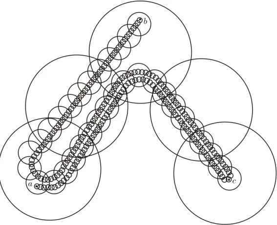
Example 4.5. Let 𝑎, 𝑏 and 𝑐 be distinct points in the plane. It is easy to construct simple chains 𝒞𝑛 = (𝐶
1, . . . , 𝐶𝑘𝑛), 𝑛 = 1, 2, . . . whose links are discs of diameter < 2
−𝑛 satisfying conditions
below:
1. For each 𝑛 = 1, 2, . . . the closure of each link of 𝒞𝑛+1 is a subset of a link of 𝒞n,
2. For each 𝑛 = 1, 2, . . . , C3𝑛+1 goes from 𝑎 to 𝑐 through 𝑏, C3𝑛+2 goes from 𝑏 to 𝑐 through 𝑎, C3𝑛+3 goes from 𝑎 to 𝑏 through 𝑐.
We set 𝐾𝑛= 𝑘𝑛 ⋃︁ 𝑖=1 ¯ 𝐶𝑖𝑛 and 𝐾 = ∞ ⋂︁ 𝑛=1 𝐾𝑛
It is then easy to check that 𝐾 is irreducible between each two of the three points 𝑎, 𝑏 and 𝑐 (See Figure 4.1).
Surprisingly, “almost” every continuum is indecomposable.
Lemma 4.6. In the space 𝐶(𝐷2) of sub-continua of a the unit disc 𝐷2 (with the Hausdorff metric), the set of nondegenerate indecomposable sub-continua is a dense countable intersection of open sets (dense 𝐺𝛿).
Figure 4.1: An indecomposable continuum
Proof. Let ℐ be the set of non degenerate indecomposable continua of 𝐷2 and 𝐹𝑛 be the set of
all the sub-continua which are the union of two sub-continua 𝐴 and 𝐵 such that 𝐴 ̸⊂ 𝑉 (𝐵, 1/𝑛) and 𝐵 ̸⊂ 𝑉 (𝐴, 1/𝑛) 𝐹𝑛 is a closed subset of 𝐶(𝐷2), the set of all sub-continua of 𝐷2. Hence,
the complement of ℐ (in 𝐶(𝐷2)) can be written as ⋃︀∞𝑛=1𝐹𝑛.
Furthermore, ℐ is a dense set in 𝐶(𝐷2) Indeed, let 𝐶 ∈ 𝐶(𝐷2) and 𝜀 > 0. It is easy to
construct a polygonal arc 𝛼 in 𝐷2with 𝑑𝐻(𝛼, 𝐶) < 𝜖/2 (where 𝑑𝐻 is the Hausdorff metric). Using
the construction of Example 1, it is then possible to construct an indecomposable continuum 𝐾 such that 𝑑𝐻(𝐾, 𝐶) < 𝜀.
Example 4.7 (The Pseudo-arc). Let 𝒞 and 𝒟 be two simple chains where 𝒞 strongly refines 𝒟 (meaning the closure of each link of 𝒞 = (𝐶1, . . . , 𝐶𝑛) is contained in a link of 𝒟 = (𝐷1, . . . , 𝐷𝑚)).
We say that 𝒞 is crooked in 𝒟 provided that if 𝑘 − ℎ > 2 and 𝐶𝑖 and 𝐶𝑗 are links in 𝐷ℎ and
𝐷𝑘 of 𝐷, respectively, then there are links 𝐶𝑟 and 𝐶𝑠 of 𝒞 in links 𝐷𝑘−1 and 𝐷ℎ+1 respectively,
such that either 𝑖 > 𝑟 > 𝑠 > 𝑗 or 𝑖 < 𝑟 < 𝑠 < 𝑗.
In the plane, let 𝒞1, 𝒞2, . . . be a sequence of chains between two distinct points 𝑎 and 𝑏 such that for each 𝑛 = 1, 2, . . . we have
1. 𝒞𝑛+1 is crooked in 𝒞𝑛,
2. the diameter of each link of C𝑛 is less than 1/𝑛.
Set 𝐾𝑛= 𝑘𝑛 ⋃︁ 𝑖=1 𝒞𝑛𝑖.
Then 𝐾 =⋂︀∞𝑛=1𝐾𝑛is called a pseudo-arc. Is is an indecomposable continuum. It has the
amaz-ing followamaz-ing property. If 𝐻 is a nondegenerate sub-continuum of 𝐾, then 𝐻 is indecomposable. That is the pseudo-arc is hereditarily indecomposable.
In particular 𝐾 contained no arc. Moise [14] proved that every two pseudo-arcs are homeo-morphic and Bing [5] gave a topological characterization of the Pseudo-arc.
Let 𝑋 a continuum and 𝑥 ∈ 𝑋. The composant of 𝑥 is the union of all proper sub-continua of 𝑋 which contain 𝑥. It is also the set of all points 𝑦 such that 𝑋 is not irreducible between 𝑥 and 𝑦.
Two composants are not necessarily disjoint. For example an arc ab has exactly three composants, namely, 𝑎𝑏, 𝑎𝑏 − {𝑎} and 𝑎𝑏 − {𝑏} corresponding to 𝑥 ̸= 𝑎, 𝑏, or 𝑥 = 𝑎, or 𝑥 = 𝑏. In fact it is easy to show that every decomposable continuum is a composant for some point.
In a space which is not connected the composants are the same as the components and this notion has no interest, but this notion is very useful in the study of indecomposable continua as we will see later.
Lemma 4.8. In a nondegenerate continuum 𝑋, each composant is a dense union of a countable family of proper subcontinua.
Proof. Let 𝐶 be a composant defined by a point 𝑝 and 𝑈, 𝑉 be nonempty open sets in 𝑋 with ¯
𝑉 ⊂ 𝑈 . If 𝑝 ̸∈ 𝑉 , the closure of the component 𝑁 of 𝑋 − 𝑉 which contains 𝑝 is contained in 𝐶. But 𝑁 ∩ 𝐹 𝑟(𝑉 ) ̸= ∅ (see Exercise 4.4), so that 𝐶 ∩ 𝑈 ̸= ∅. Hence ¯𝐶 = 𝑋.
To prove that 𝐶 is a countable union of proper sub-continua of 𝑋, choose a countable basis 𝑈1, 𝑈2, . . . for 𝑋 − {𝑝} and let 𝑁𝑖 be the component of 𝑝 in 𝑋 − 𝑈𝑖 then C =
⋃︀
𝑖𝑁𝑖.
Corollary 4.9. Every composant of an indecomposable continuum has empty interior.
The proof is a straightforward application of Baire’s theorem. In fact it is easy to verify, the following.
Lemma 4.10. If a continuum has a composant with empty interior then it is in decomposable. Lemma 4.11. If 𝑋 is an indecomposable continuum, the composants of 𝑋 partition 𝑋 and there are uncountably many of them.
Proof. Let 𝐶1 and 𝐶2 be two composants defined respectively by the points 𝑝1 and 𝑝2 and
suppose that there exists 𝑥 ∈ 𝐶1∩ 𝐶2. Then we can find
∙ a proper sub-continuum 𝐾1 ⊂ 𝐶1 such that 𝑥, 𝑝1 ∈ 𝐾1,
∙ a proper sub-continuum 𝐾2 ⊂ 𝐶2 such that 𝑥, 𝑝2 ∈ 𝐾2 .
Thus 𝐾 = 𝐾1 ∪ 𝐾2 is a proper sub-continuum of 𝑋. Let 𝑦 be any point of 𝐶1. There
exists a proper sub-continuum 𝐾3 ⊂ 𝐶1 such that 𝑦, 𝑝1 ∈ 𝐾3, thus 𝐾′ = 𝐾 ∪ 𝐾3 is a proper
sub-continuum of 𝑋 and therefore 𝑦 ∈ 𝐶2. Hence, 𝐶1 ⊂ 𝐶2 and similarly 𝐶2⊂ 𝐶1.
Suppose there are at most a countable many distinct composants. Then 𝑋 =⋃︀𝑛𝐶𝑛 is also
an at most countable union of proper sub-continua, each of which having empty interior. But this is not possible by Baire’s theorem.
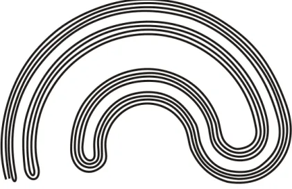
Example 4.12 (Knaster’s Continuum). We begin with the Cantor middle-third set 𝐶. Then we add to 𝐶 all the semicircles lying in the upper half plane with center at (1/2, 0) that connect each pair of points in the Cantor set that are equidistant from 1/2. Next we add all semicircles in the lower half plane which have for each 𝑛 ≥ 1 centers at (5/(2 · 3𝑛), 0) and pass through each point in the Cantor set lying in the interval
The resulting set is partially depicted in Figure 4.2. The fact that this set is indecomposable results from the following observation [11]. The composant of the origin is the curve obtained by starting from the origin and then following successively all the successive semicircles. This curve has empty interior.
Figure 4.2: Knaster’s Continuum
We are now going to describe another way to look at continua, namely via inverse limits. This gives in some case, a parametrization of a continuum by a simpler space.
Let (𝑋, 𝑑) be a metric space and 𝑓 : 𝑋 → 𝑋 a continuous map, the inverse limit space, (𝑋, 𝑓 ) is the space
(𝐾, 𝑓 ) = {x = (𝑥0, 𝑥1, . . . ); 𝑥𝑛∈ 𝑋 and 𝑓 (𝑥𝑛+1) = 𝑥𝑛for all 𝑛 ≥ 0}
with metric d given by
d(x, y) = ∞ ∑︁ 𝑛=0 𝑑(𝑥𝑛, 𝑦𝑛) 2𝑛 .
If 𝑋 is a continuum, then (𝑋, 𝑓 ) is also a continuum. The map 𝑓 induces a homeomorphism ˆ
𝑓 : (𝑋, 𝑓 ) → (𝑋, 𝑓 ) given by
ˆ
𝑓 ((𝑥0, 𝑥1, . . . )) = (𝑓 (𝑥0), 𝑥0, . . . )
from which the inverse is just the usual shift map.
Lemma 4.13. Let 𝑋 be a continuum and 𝑓 : 𝑋 → 𝑋 be a surjective continuous map such that whenever 𝑋 = 𝐴 ∪ 𝐵 where 𝐴 and 𝐵 are sub-continua of 𝑋, we have 𝑓 (𝐴) = 𝑋 or 𝑓 (𝐵) = 𝑋. Then, (𝑋, 𝑓 ) is an indecomposable continuum.
Proof. Let 𝑋∞ = (𝑋, 𝑓 ) and suppose there exist two sub-continua 𝐴∞ and 𝐵∞ of 𝑋∞ with
𝑋∞= 𝐴∞∪ 𝐵∞. Let 𝜋𝑛 : 𝑋∞→ 𝑋 be the natural projection onto the nth coordinate. From
the relation 𝜋𝑛(𝑋∞) = 𝜋𝑛(𝐴∞) ∪ 𝜋𝑛(𝐵∞) = 𝑋 for all 𝑛 ≥ 0, and from the property of 𝑓 , it
follows that there are infinite many 𝑛 for which we have, say 𝜋𝑛(𝐴∞) = 𝑋. It follows then from
the relation 𝑓𝑛∘ 𝜋𝑛+1= 𝜋𝑛 which is true on 𝑋∞, that 𝜋𝑛(𝐴∞) = 𝑋 for all 𝑛 ≥ 0. Hence 𝐴∞ is
dense in 𝑋∞and thus 𝐴∞= 𝑋∞.
Remark 4.14. The preceding lemma is still true if we replace the hypothesis of the lemma by the weaker one : there exists 𝑁 > 0 such that for all sub-continua 𝐴, 𝐵 of 𝑋 such that 𝑋 = 𝐴 ∪ 𝐵, then 𝑓𝑁(𝐴) = 𝑋 or 𝑓𝑁(𝐵) = 𝑋.
Example 4.15 (The Solenoid). Let 𝑋 = 𝑆1, the unit circle and 𝑓 : 𝑆1 → 𝑆1 the map given
by 𝑓 (𝜃) = 𝑝𝜃 (𝑝 ≥ 2). Then (𝑋, 𝑓 ) is an indecomposable continua which is called the p-adic solenoid Σ𝑝. There is a natural group structure on Σ𝑝 inherited from the one on 𝑆1. We can
deduce from this fact that Σ𝑝 is homogenous (meaning that from any two points there is a
homeomorphism of Σ𝑝 onto Σ𝑝 taking one of these point to the other). We can show also that
each proper sub-continuum of Σ𝑝 is an arc. It is interesting to note that the last two properties
actually characterize solenoid [8].
A continuum Λ which separates the plane into exactly two components and which is ir-reducible with respect to this property will be called a cofrontier. Let 𝑈𝑖 be the bounded
complementary domain of Λ and 𝑈𝑒 be the unbounded one. Then 𝐹 𝑟(𝑈𝑖) and 𝐹 𝑟(𝑈𝑒) are
sub-continua of Λ which separate the plane thus, 𝐹 𝑟(𝑈𝑖) = 𝐹 𝑟(𝑈𝑒) = Λ. Conversely, if a plane
continuum Λ separates the plane into exactly two complementary domains and is there common frontier, then Λ irreducibly separates the plane and is therefore a cofrontier.
Remark 4.16. Indecomposable continuum have been discovered by Brouwer to show that Schoen-flies’ conjecture that every cofrontier could be decomposed into the union of two proper subcon-tinua was wrong.
Figure 4.3: Wada Lakes
Note that a continuum which is the common boundary of two simply connected domains is not necessary a cofrontier as we will see below. The first explicit example of a such continuum was reported in a paper by Yoneyama in 1917 [23]. This beautiful example is known as the Lakes of Wada continuum. In his paper Yoneyama states that the example was reported to him
by a Mr. Wada, but no one seems to know anything else about Mr. Wada. In 1924, Kuratowski [11] proved that if 𝐾 is a plane continuum is the common boundary of more than 3 disjoint open sets then 𝐾 is either indecomposable or the union of two indecomposable continua.
To preserve the poetic flavour of the original example [9], we take a double annulus, as shown in Figure 4.3, to be a island in the ocean with two lakes, one having blue water and the other red water. At time 𝑡 = 0, we dig a canal from the ocean, which brings salt water to within a distance of 1 unit of every point of land. At time 𝑡 = 1/2, we dig a canal from the blue lake, which bring blue water to within a distance 1/2 of every point of land.At time 3/4, we dig a canal to bring red water to within a distance of 1/3 at every point of land. A time 𝑡 = 7/8, we dig a canal from the end of the first canal to bring salt water to within a distance 1/4 of every point of land and so forth. If we think of these canals as open sets, at time 𝑡 = 1, the “land” remaining is a plane continuum which bounds three open domains in the plane.
Exercises
Exercise 4.1. In Theorem 4.5, give a meaning to the statement “the simple chains are as straight as possible in each other” (see the construction of the arc in the proof of theorem 3.8). Obtain, this way, an indecomposable continuum such that every of its proper nondegenerate sub-continua is an arc.
Exercise 4.2. Show thatTheorem 4.7 (the Pseudo-arc) is hereditarily indecomposable. Exercise 4.3. Show that most of the sub-continua of a closed 2-cell are hereditarily indecom-posable.
Exercise 4.4. Let 𝑋 be a continuum, 𝑈 an open set of 𝑋 and 𝑁 a component of 𝑈 . Then, ¯
𝑁 ∩ 𝐹 𝑟(𝑈 ) ̸= ∅.
Chapter 5
Attractors and Indecomposable
Continua
Let 𝑋 be a compact metric space and 𝑓 : 𝑋 → 𝑋 a continuous map. A nonempty compact subset Λ ⊂ 𝑋 is an attractor for 𝑓 if there is an open neighbourhood 𝑈 of Λ such that 𝑓 (𝑈 ) ⊂ 𝑈 and
Λ = ⋃︁
𝑛≥0
𝑓𝑛( ¯𝑈 ).
An attractor is clearly an invariant set for 𝑓 (𝑓 (Λ) = Λ). There are other definitions of attractors in common use, but this one is perhaps the simplest. However this definition suffers the defect that it does not produce a single, indecomposable attractor To remedy this, we introduce the following terminology Λ is a transitive attractor for 𝑓 if 𝑓 is topologically transitive on Λ, that is for any pair of open sets 𝑈, 𝑉 ⊂ 𝑋 there exist 𝑘 > 0 such that 𝑓𝑘(𝑈 ) ∩ 𝑉 ̸= ∅.
Given a point 𝑝, the stable set of 𝑝 is given by
𝑊𝑠(𝑝) = {𝑧 ∈ 𝑋; 𝑑(𝑓𝑛(𝑝), 𝑓𝑛(𝑧)) → 0 as 𝑛 → +∞} .
Equivalently, a point 𝑧 lies in 𝑊𝑠(𝑝) if 𝑝 and 𝑧 are forward asymptotic. Similarly, we define the unstable set of 𝑝 to be
𝑊𝑢(𝑝) =⌋︀𝑧 ∈ 𝑋; 𝑑(𝑓−𝑛(𝑝), 𝑓−𝑛(𝑧)) → 0 as 𝑛 → +∞{︀.
We say that a periodic point of 𝑓 (ie a point 𝑝 for which there exists 𝑛 > 0 with 𝑓𝑛(𝑝) = 𝑝) is stable (resp unstable) if 𝑊𝑠(𝑝) (resp 𝑊𝑢(𝑝)) is a neighbourhood of 𝑝. See [7], for a beautiful introduction to Dynamical Systems
Example 5.1 (The Horseshoe Map). Let 𝑆 be the square 𝐼 × 𝐼 where 𝐼 = [0, 1], and let 𝐷 be the two dimensional disc 𝐷 = 𝑆 ∪ 𝐴 ∪ 𝐵 where 𝐴 and 𝐵 are half disc attached to opposite sides {0} × 𝐼 and {1} × 𝐼 of the square 𝑆 as depicted inFigure 5.1.
The standard horseshoe map 𝐹 takes 𝐷 inside itself according to the following prescription. First, linearly contract 𝑆 in the vertical direction by a factor 𝛿 < 1/2 and expand it in the horizontal direction by a factor 1/𝛿 so that 𝑆 is long and thin. Then put 𝑆 back inside 𝐷 in a horseshoe shaped figure as in Figure 5.2. The semicircular regions 𝐴 and 𝐵 are contracted and mapped inside 𝐴 as depicted. We remark that 𝐹 (𝐷) ⊂ 𝐷 and that 𝐹 is one-to-one. However, since 𝐹 is not onto, 𝐹−1 is not globally defined.
Now let 𝜋 : 𝐷 → 𝐼 given by 𝜋(𝐴) = {0}, 𝜋(𝐵) = {1} and 𝜋((𝑥, 𝑦)) = 𝑥 for all (𝑥, 𝑦) ∈ 𝑆 = 𝐼 × 𝐼. The map 𝐹 has the following properties:
1. 𝐹 (𝜋−1(𝜋(𝑧))) ⊂ 𝜋−1(𝜋(𝐹 (𝑧))) for all 𝑧 ∈ 𝐷, 2. 𝐹 (𝐴) ⊂ 𝑖𝑛𝑡(𝐴) and 𝐹 (𝐵) ⊂ 𝑖𝑛𝑡(𝐴),
Figure 5.1: Building the Horseshoe
Figure 5.2: The Horseshoe
3. For all 𝑥 ∈ 𝐼, 𝜋−1(𝑥) ∩ 𝐹 (𝐷) has exactly two components, 4. diam(𝐹𝑛(𝜋−1(𝜋(𝑧))) → 0 uniformly in 𝑧 ∈ 𝐷 as 𝑛 → +∞.
The attractor for the horseshoe map 𝐹 is the set Λ𝐻 =
⋂︁
𝑛≥0
𝐹𝑛(𝐷).
It is possible to show that Λ𝐻 is homeomorphic to Knaster’s continuum (Theorem 4.12).
How-ever, we are going to show the indecomposability of Λ𝐻 by other means.
𝐹 induces a continuous map of the interval 𝑓 : 𝐼 → 𝐼 defined by 𝑓 (𝑥) = 𝜋(𝐹 (𝜋−1(𝑧))). The map 𝑓 has the following properties 𝑓 (0) = 𝑓 (1) = 0 and there exist 0 < 𝑎1< 𝑎2 < 𝑎3 < 𝑎4 < 1
such that 𝑓 is strictly increasing on [𝑎1, 𝑎2], 𝑓 is strictly decreasing on [𝑎3, 𝑎4], 𝑓 ([0, 𝑎1]) =
𝑓 ([𝑎4, 1]) = {0} and 𝑓 ([𝑎2, 𝑎3]) = {1} (see Figure 5.3).
Theorem 5.2. Let ˆ𝜋 : Λ𝐻 → (𝐼, 𝑓 ) defined by
ˆ
𝜋(𝑧) = (𝜋(𝑧), 𝜋(𝐹−1(𝑧)), . . . ).
Then ˆ𝜋 is a homeomorphism such that 𝐹 ∘ ˆ𝜋 = ˆ𝑓 ∘ ˆ𝜋. That is, 𝐹|Λ𝐻 and ˆ𝑓 are topologically
conjugate.
Proof. The following proof is due to Barge [3]. Since
Figure 5.3:
we see that ˆ𝜋(𝑧) is indeed an element of (𝐼, 𝑓 ). ˆ
𝜋 is clearly continuous. To see that ˆ𝜋 is one-to-one and onto, let x = (𝑥0, 𝑥1, . . . ) ∈ (𝑋, 𝑓 )
and let
𝐶𝑛= 𝐹𝑛(𝜋−1(𝑥𝑛)) for 𝑛 = 0, 1, . . .
Then 𝐶𝑛 is a closed, nonempty subset of 𝐷 for each 𝑛 ≥ 0, and since
𝐹 (𝜋−1(𝑥𝑛+1)) ⊂ 𝜋−1(𝑓 (𝑥𝑛+1)) = 𝜋−1(𝑥𝑛),
we have 𝐶𝑛+1 ⊂ 𝐶𝑛 for all 𝑛 ≥ 0. Thus
⋂︀
𝑛≥0𝐶𝑛 is a nonempty compact set. But since
diam(𝐶𝑛) → 0 as 𝑛 → +∞ (condition (4)), we have
⋂︀
𝑛≥0𝐶𝑛 = {𝑧} is a singleton. Now if
𝑧 ∈⋂︀𝑛≥0𝐶𝑛, then
𝜋(𝑧) = 𝑥0, 𝜋(𝐹−1(𝑧)) = 𝑥1, . . .
That is, ˆ𝜋(𝑧) = x, but then 𝑧 must be in ⋂︀𝑛≥0𝐶𝑛. ˆ𝜋 is one to one as well as onto.
It follows then from Lemma4.13 that Λ𝐻 is an indecomposable continuum. We note also,
that 𝑓 has two unstable fixed point 𝑝0 and 𝑝1 and one stable fixed point 0. These points
correspond to fixed points for ˆ𝑓 , p0 = (𝑝0, 𝑝0, . . . ) and p1 = (𝑝1, 𝑝1, . . . ) and thus to fixed
points for 𝐹 in 𝑆. Given an arbitrary point 𝑥 ∈ 𝐼, there exists a unique 𝑥1 ∈ [𝑎1, 𝑎2] such
that 𝑓 (𝑥1) = 𝑥, then a unique 𝑥2 ∈ [𝑎1, 𝑎2] such that 𝑓 (𝑥2) = 𝑥1 and so on. In this way,
we construct a sequence x = (𝑥, 𝑥1, 𝑥2, . . . ) ∈ (𝑋, 𝑓 ) with the property that ˆ𝑓−𝑛(x) → 0 as 𝑛
→ +∞. Moreover, since ˆ𝑓 (𝑊𝑢(p0)) ⊂ 𝑊𝑢(p0), this shows that 𝑊𝑢(p0) is dense in Λ𝐻.
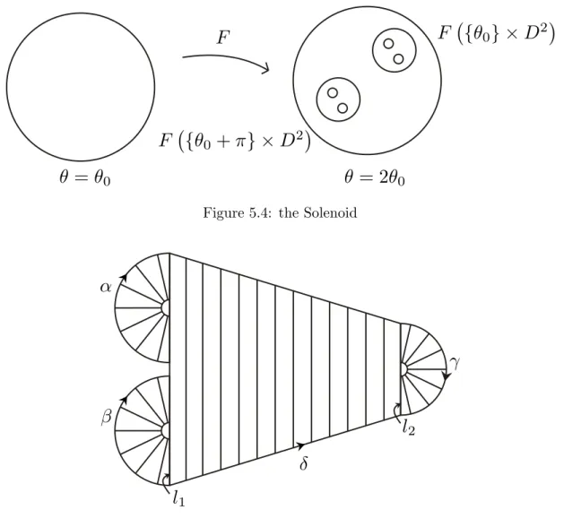
Example 5.3 (The Solenoid from dynamical viewpoint). Let 𝑇 = 𝑆1× 𝐷2 be a solid torus in R3
and consider the map
𝐹 (𝜃, 𝑥) = (2𝜃, 1 10𝑥 +
1 2𝑒
2𝜋𝑖𝜃)
where 𝑥 ∈ 𝐷2 and 𝜃 ∈ 𝑆1. Globally, 𝐹 may be interpreted as follows. In the 𝜃 coordinate, 𝐹 is simply the doubling map 𝜃 ↦→ 2𝜃. In the 𝐷2-direction, 𝐹 is a strong contraction, with image a disc whose center depends on 𝜃. Thus the image of 𝑇 is another solid torus inside 𝑇 which wraps twice around 𝑇 (see Figure 5.4).
Figure 5.4: the Solenoid
Figure 5.5: the Plykin attractor
We set Λ𝑆 =
⋃︀
𝑛≥0𝐹𝑛(𝑇 ). Let 𝜋 : 𝑆1× 𝐷2 → 𝑆1 be the projection onto the first factor. We
can show as in the case of the horseshoe map that the induced map ˆ𝜋 : Λ𝑆 → (𝑆1, 𝑔) given by
ˆ
𝜋(𝑧) = (𝜋(𝑧), 𝜋(𝐹−1(𝑧)), . . . ).
where 𝑔 : 𝜃 ↦→ 2𝜃 gives a conjugacy between 𝐹 on Λ𝑆 and ˆ𝑔 on (𝑆1, 𝑔). This construction gives
us also a way to embed the solenoid Σ2 defined in Theorem 4.12into the 3-space 𝑅3.
In fact, the inverse limit construction works well for a class of attractors known as “expand-ing” attractors. These attractors are characterized by uniform expansion within the attractor itself. As in the case of the solenoid, such attractors can be suitably modeled by an inverse limit of a lower dimensional expanding map like 𝜃 ↦→ 2𝜃 on 𝑆1.
The main difference is that the model space is more complicated than 𝑆1 ; usually it is a “branched one-manifold”, a continuum which is the union of a finite number of arcs each of which intersecting by pairs only in there endpoints. This concept was introduced by Williams [22]. He showed that every hyperbolic, one-dimensional, expanding attractor for a discrete dynamical system is topologically conjugate to the induced map on an inverse limit space based on a branched one-manifold. We will illustrate it via an example of an attractor due to Plykin. Rather than give a formula for this map, we will define it geometrically, as we did it for the horseshoe.