Mesoscale structure and dynamics of the tropical tuna's associated-environment in the Indian and the Eastern Pacific Oceans : comparative approach

(1)

HAL Id: tel-03217624

https://tel.archives-ouvertes.fr/tel-03217624

Submitted on 5 May 2021

HAL is a multi-disciplinary open access

archive for the deposit and dissemination of sci-entific research documents, whether they are pub-lished or not. The documents may come from teaching and research institutions in France or abroad, or from public or private research centers.

L’archive ouverte pluridisciplinaire HAL, est destinée au dépôt et à la diffusion de documents scientifiques de niveau recherche, publiés ou non, émanant des établissements d’enseignement et de recherche français ou étrangers, des laboratoires publics ou privés.

Mesoscale structure and dynamics of the tropical tuna’s

associated-environment in the Indian and the Eastern

Pacific Oceans : comparative approach

Carmen Liliana Roa Pascuali

To cite this version:

Carmen Liliana Roa Pascuali. Mesoscale structure and dynamics of the tropical tuna’s associated-environment in the Indian and the Eastern Pacific Oceans : comparative approach. Ecosystems. Université Montpellier, 2016. English. �NNT : 2016MONTS030�. �tel-03217624�

(2)

Mesoscale structure and dynamics of the

tropical tuna’s associated-environment in the

Indian and the Eastern Pacific Oceans;

comparative approach

Structure de méso-échelle et dynamique de

l'environnement des thonidés tropicaux dans

l’Océan Indien et l’Océan Pacifique Est ;

approche comparative

Délivré par l’Université de Montpellier

Préparée au sein de l’école doctorale SIBAGHE

Et de l’unité de recherche MARBEC

(IRD / IFREMER /

Université de Montpellier / CNRS)

Spécialité : ÉCOSYSTÈMES

Présentée par Carmen Liliana ROA PASCUALI

Soutenue le 15 janvier 2016 devant le jury composé de

M. Martin HALL, Professeur des Universités, IATTC Rapporteur M. Alexis CHAIGNEAU, Chargé de Recherche, IRD (UMR LEGOS) Rapporteur M. Daniel GAERTNER, Chargé de Recherche, IRD (UMR MARBEC) Examinateur M. Jacques PANFILI, Chargé de Recherche, IRD (UMR MARBEC) Examinateur M. Hervé DEMARCQ, Chargé de Recherche, IRD (UMR MARBEC) Directeur de thèse

(3)

(4)

To my family,

To my daughter Manuela "tuti"

who came to my life to teach me what is the true love about.

(5)

(6)

Abstract

This study provides an approach to the comprehension of the mesoscale structures in the habitat of three major tropical tunas species, yellowfin (Thunnus albacares; YFT), skipjack (Katsuwonus pelamis; SKJ) and bigeye (Thunnus obesus: BET). These species, mainly caught by the purse seiner's fishery worldwide, represent 20% and 13% of the world total production for the Indian Ocean (IO) and the Eastern Pacific Ocean (EPO) respectively. Single set records from this fishing gear in both oceans, were used to separately evaluate the environmental characteristics of their fishing grounds for three fishing modes: free school (FS), log (LOG) and fish aggregating devices (FADs) and several fish sizes. Prior to the analyses, a statistical and expert-based method was applied to detect and classify thermal fronts at basin scale whereas distances of tuna catch positions to eddy structures (anticyclonic and cyclonic) were calculated based on the detection method of winding angle. We found that strong fronts are mostly found in coastal regions and weak fronts in the open ocean. The consideration of the frontal occurrence and intensity helps to spatially differentiate mechanisms of frontogenesis than may attract tunas. We also observed clear differences about distances, between eddies and tunas catch positions depending on fish-size.

In addition to these mesoscale components, other categories of variables as classic, temporal and fishery-related ones were added to describe the environment of the fishing grounds, based on tuna catch locations. We then used the Boosted Regression Tree (BRT) method to create a three step modeling scheme for each study area, first to explore the responses of the catch level and fish-size to the different fishing modes; then to consider the effect of simulated randomly distributed catch positions, in order to estimate the mesoscale effects; finally to explore the relative dominance of each species. We globally found similar results than previous ones obtained at catch level.

All BRT models showed that the catch level was better explained by the environmental conditions on free school (FS) than on FADs and that differences regarding environment-tuna distribution were more important among fish-sizes than among species. We quantified for the first time the dominant influence of the mesoscale in determining tuna's habitat, confirmed by the poor explanation obtained all “random catch” models, mainly for the IO. For both oceans, small-sized individuals were strongly related with the proximity to mesoscale eddies (<200 km) whereas the large-sized individuals were found at larger distances. A strong influence of mesoscale fronts was observed mainly in the EPO and in the IO only in the coastal regions where strong fronts become important.

In the EPO different environmental conditions were observed in three well defined sub-regions as the Peru coastal upwelling, the Equatorial Tongue, and the Costa Rica Dome. Contrarily to the IO were the fishing grounds were relatively homogeneous in terms of Sea Surface Temperature (SST) and Sea surface Concentrations (SSC) these two parameters highly influence the tuna distribution in the EPO. In general for the this ocean, the total percentage of relative contribution by category of variables for the entire modeling scheme was 34% for the mesoscale variables, 39% for the classic variables and 27% for the temporal and fishery-related variables. For the EPO, even if the mesoscale category remains important (37%), the most relevant contributions were found for the classic variables with 55% whereas 8% was observed for the temporal component.

Key words: Tropical tunas, Indian Ocean, Eastern Pacific Ocean, mesoscale, purse seiner, species, fish-size,

(7)

(8)

Résumé

Le présent travail a pour but d'étudier la structuration à méso-échelle (de quelques kilomètres à quelques centaines de kilomètres) de l'environnement marin des trois espèces majeures de thons tropicaux, l'Albacore (Thunnus Albacares), le Listao (Katsuwonus Pelamis) et le thon obèse (Thunnus obesus), pêchés à la seine tournante dans les océans Indien (OI) et Pacifique Tropical Est (OPE), en fonction de leur tailles et leur distribution. Ces trois espèces représentent 20% et 13% des prises mondiales respectivement dans les 2 océans. Les prises par calées uniques sont utilisées pour évaluer séparément les caractéristiques environnementales de leur zones de pêche pour trois modes de pêche: sur banc libre (FS), objets flottants naturels (LOG) et sur dispositifs de concentration du poisson (DCP), ceci pour plusieurs tailles d'individus.

Préalablement aux analyses, une double méthode statistique et d'expertise est développée pour la détection et la classification des fronts thermiques à l'échelle des bassins océaniques, tandis que les tourbillons de méso-échelle, cycloniques et anticycloniques sont détectés par la méthode des winding angle. Les distances des prises à ces structures sont ensuite calculées. Nous trouvons que les fronts intenses concernent surtout les régions côtières et les fronts faibles l'océan du large, ce qui permet de considérer différents mécanismes de frontogénèse pouvant avoir un pouvoir attractif différent sur les thons.

En plus des composantes de méso-échelle, les variables classiques de l’environnement, les variables temporelles et celles liées à la pêche sont utilisées. Nous utilisons le modèle bayésien " Boosted Regression Tree” (BRT) suivant un schéma en 3 phases pour chaque océan pour explorer les réponses du niveau de prise pour chaque espèce et trois modes de pêche. La dominance relative est également explorée pour les prises sur FADs (O.I) et FADs et FS (OPE) et montre des résultats similaires au niveau de prise.

Tous les modèles BRT montrent que le niveau de prise est davantage relié à la variabilité environnementale pour les bancs libres que pour les FADs. Nous mettons en évidence pour la première fois l'importance des structures de méso-échelle sur la définition des habitats des thons, ce qui est confirmé par les faibles niveaux d'explication obtenus par les modèles de type « random », notamment dans l'océan indien. Pour les deux océans, les petits individus sont fortement associés aux tourbillons (distances <200km) tandis que les plus gros sont situés plus loin des tourbillons.

Une faible influence des fronts thermiques est constatée dans l'Océan Indien tandis que l'opposé est trouvé pour le Pacifique, sauf dans les régions côtières où les forts fronts ont une influence prépondérante. Différentes conditions environnementales sont observées dans des régions précises du Pacifique comme celles d'upwelling côtier, la bande équatoriale et le dôme du Costa Rica. Contrairement à l'Océan Indien, où les zones de pêches sont relativement homogènes en terme de température et chlorophylle de surface, ces deux paramètres influencent nettement plus la distribution des thons dans le Pacifique. Dans l'Océan Indien, le pourcentage total des contributions relatives par catégories de variables est de 34 % pour les variables de méso-échelle, de 39 % pour les variables classiques et de 27 % pour les autres (temporelles et pêche). Pour le Pacifique Est, même si la méso-échelle est importante (37%) les autres variables dominent en contribution relative (55 % et 8%).

Mots clé : Thons tropicaux, taille, Océan Indien, Océan Pacifique Est, environnement, méso-échelle, senne

(9)

(10)

Acknowledgments

“We don't meet people by accident. They are meant to cross our path for a reason”

(Unknown)

A

t this moment, when I am getting to the end of this PhD journey I truly believe that perseverance is the secret. If you continue working without giving up -despite the adversities- suddenly the magic happens, everything has a meaning and the right people appear around you. They are those that will help you day by day to reach your goal, they will -literally- put in your hands one by one of the strips of wood and the nails that you need to build the ship in which you and your fulfilled aim will be sailing. Once the ship finished, the satisfaction is not only to see how it raises on the sea but also to see all and each one of the sailors who will be navigating with you by the rest of your life. They are the same that had helped you building that beautiful ship, those that trusted in you and encourage you now to make the trip. To every sailor, thank you, without you this had not been possible. If I forget to mention someone here, that is not a problem, you know that your names are already registered in the “log book” and that we are ready to navigate!

Before continue, I want to express my gratitude to the one that can do everything, the one that lifts you each time that you fall, the one that loves you in spite of your faults, the one that really knows your heart

and to knows everything what you are capable to do, Thanks to God.

First and foremost I wish to thank my thesis advisor, Hervé Demarcq who trusted in me from the beginning. Thank you for your generosity sharing your knowledge, for your dedication, time and patience. Thanks a lot for supported me not only by providing a research assistantship over all these years, but also academically and emotionally through the rough road to finish this thesis.

Besides my advisor, I would like to thank all the members of the thesis committee, Doctor Daniel Gaertner thank you for your trust and your willingness answering all my questions, thank you for opening the doors to the collaborations done and for your recommendations. Doctor Alexis Chaigneau thank you for providing me with the oceanographic data derived from your useful methods and for your important remarks to this document. Doctor Alain Fonteneau thank you for your helpful comments and the very precise questions that improved this study. Doctor Jacques Panfili thank you for your time, willingness and your advice. I am especially grateful to Doctor Martin Hall, who arranged his agenda many times to be in France to support the development of this work and who provided me the opportunity to join their team at the Inter-American Tropical Tuna Commission (IATTC) as intern. Thank you for having accepted to be part of this study, for your trust, your very constructive comments, for being attentive to listen my questions and to open my mind to the specific details of the fisheries in the Pacific Ocean. I want to thank you also for motivating me to meet new researchers and to know about new oceanographic methods. Thank you for encouraging me

(11)

to present my results everywhere (Colombia, USA and France). Thank you for having introduced me to the people at NOAA and ESR labs. Finally thanks for teaching me to believe in my ideas and skills and for always consider my suggestions.

My sincere thanks also to the director of the IATTC Doctor Guillermo Compean, who approved the collaboration proposed and my stay in La Jolla. Also thanks to all IATTC staff for the collaboration, specially to Marlon Roman, Nick Vogel, Carolina Minte Vera and to Marisol Aguilar. Also thanks to the people whom I had the pleasure to share with during in California, Karen, Gaston, Xochilt, Alain, thanks for the warm environment, for providing me a nice home and for your friendship.

Igratefully acknowledge Doctor Francisco (Cisco) Werner and Doctor Paul Fiedler, from NOAA, for their time and important comments and suggestions. Also thanks to Doctor Yi Xu for your advice about statistical modeling. I am also grateful to Doctor Kathleen Dohan who gave me the opportunity to work with her at ESR in Seattle, for your time and willingness, for teaching me the functioning of OSCAR model, also thank you very much for your advice and perspectives for the future.

In Sète I want to thank the Observatoire thonier, mainly to Pierre Chavance, Emmanuel Chassot and Pascal Bach for the access to the data bases and for funding the final months of my PhD. Also thanks to Laurent Floch, Pascal Cauquil and Alain Damiano for the data, for the interviews with the observers and the explanations about the dynamics of the french purse seine tuna fleet.

An special acknowledgment goes to my great friends and colleagues, Doctor Karen Nieto thanks for your sense of humor, your positive energy, motivation and your strong technical collaboration. To Isabel Terrier, Isa thanks for your kindness, for sharing your home with me several times, in Sète and in Paris, for your kind words, your trust and overall for your interest to keep alive our friendship despite the distance . Also thanks to my office mate of all these years, Doctor Sibylle Dueri a true friend ever since we began to share an office. Thank you for the nice conversations, for sharing tips about maternity, for your big heart, for your autonomy, discipline and dedication to work that I deeply admire. I also want to thank to my old friend Paola Sandoval -part of our “Marine Biology's soccer team” in Colombia- for be my sister in France, to had encouraged me to continue and for remembered me who I was and who I have to continue being now. Thanks to Manuela Capello for the motivation and support for the afternoon “promenade” with our babies. I thank with all my heart to all these valuable women for being with me during the most difficult moments.

I want to express my sincere gratitude to my good friend Norbert Billet and his family to be the support needed in the last and most critical moments of this PhD journey. Thanks for loving my daughter, Mana, for letting her share with you and for being her babysitter on weekends. Thank you for the warm food when I didn't have time to cook, for providing us a warm home in winter, for the confidence, the company and the moral support. Thanks a lot for many more things very difficult to define -because their value is difficult to quantify!-. Thanks a lot for your selflessness friendship, in a few words thanks for being our family in Sète.

I warmly thank to the Unit of research EME, today MARBEC, I'd like to start to thank the directors Doctor Philippe Cury (EME) and Laurent Dagorn (MARBEC), who had welcomed and had supported this

(12)

doctorate. I also want to thank my fellow MARBECmates, Beenesh Motah and Emmanuelle Dortel, Andrea Thiebault, Justin Amande and his family, Jeanne Fortilus, Louis Dubuisson, Lysel Garavelli, Iker Zudaire for the good moments and friendship. Giannina Passuni, Ana Alegre, Rocio Joo, Daniel Grados for the excellent Peruvian food and for the musical exchange. Also I want to thank the all Unit for the “conférences des jeudis”, for the coffee breaks and the “sardine parties” and to thanks the administrative staff, specially to Ghislaine Puget always worried for the well being of all the students.

I want to take a moment to thank to my Colombian friends Julian Uribe, Sonia Bernal, Andrea Reyes, Carlos Varon, Diva Quintero for their interest, kind words and motivation. I'm sure that life will give us the opportunity to share soon and personally, all our achievements.

Besides the people, I also want to acknowledge the institutions that founding this PhD, the Colombian Institute of Credit and Technical foreign studies (ICETEX), the COLFUTURO foundation, the Institute of Research for the Development (IRD) and the Tuna observatory (IRD, UMR MARBEC).

Last but not less important I want to thank and dedicate this work to my family. To my parents, my brothers and my sister, you are my best friends. Thank you for your unconditional support and blind confidence in my dreams, many times just moved for the enthusiasms in my eyes. Thanks to Juanito, my father, for believe and for invest in me. Thanks for giving me the wings that I needed in the middle of a convulsed time in our country where the most important thing was to learn how to survive instead to have dreams. Thanks to Edna, my mother, because with her example she taught me the value of a free-thinking woman, honest, disciplined and capable, all useful tools to face the challenges of a world full of experiences and new cultures. Thank you to my sister Margarita (Nenita) and my brother Andres (Chu) to be my “grounding”, your words, your moral and economic support has helped me to be where I am. Thanks to Yova and Dieguito (y Amparo) for always make me laugh, for question me -at the same time- about my objectives and for encourage my decisions. Thanks to mi niece Cami for your tender interest and for sharing Paris with me her first time!.

Thanks to my daughter Manuela “Tuti” for being the lighthouse that illuminated my path when everything was complete darkness. Thank you, my angel, for having showed me the strength that I never thought that I had or that I am capable to develop. Thanks for teaching me the material of which the real human beings are made of. Thanks for teaching me what is the true love about but the most important thing, thank you for choosing me to be your mother.

(13)

Agradecimientos

“No conocemos a las personas por accidente, ellas se cruzan en nuestro camino por una razón”

(Anonimo).

E

n este momento, cuando llego al final de esta etapa, creo firmemente que en la perseverancia esta el secreto. Si continuas sin desfallecer -a pesar de las adversidades- sin darnos cuenta llega ese momento mágico en que lo necesario ocurre y las personas indicadas aparecen a tu alrededor. Son estas personas las que te ayudaran a alcanzar tu meta, ellas te irán pasando -literalmente- uno a uno los listones de madera y los clavos que necesitas para construir al barco en el que navegaras con tu objetivo cumplido. Una vez terminado, la verdadera satisfacción, ademas de ver como su imponente figura se alza sobre el mar, es ver cada a uno de los marineros que navegaran contigo por el resto de tu vida. Ellos son los mismos que te ayudaron a construir el barco, que confiaron en ti sin desfallecer y te animan ahora a emprender el viaje. A todos y cada uno de ellos, gracias, sin ustedes esto no hubiera sido posible, si olvido mencionar algún nombre eso no es un problema, ustedes saben que todos están inscritos hace tiempo en la bitácora de navegación!.

Primero que todo quiero agradecer al que todo lo puede, al que te levanta cuantas veces te tropieces y caigas, al que te ama a pesar de tus defectos, al que conoce tu corazón y sabe de todo lo que eres capaz,

Gracias a Dios.

Mi mas sincero agradecimiento a mi director de tesis Hervé Demarcq, quien confió en mi desde el inicio. Gracias por su generosidad al compartir su conocimiento, por su tiempo, dedicación y paciencia. Muchas gracias por apoyarme todos estos años no solo en investigación sino academicamente y emocionalmente especialmente a través del difícil camino hacia el final de la tesis.

Quiero agradecer también a todos los miembros del comité de tesis, al Doctor Daniel Gaertner por la confianza, gentileza y buena disposición para responder mis preguntas, gracias por abrir las puertas a las colaboraciones hechas, por los contactos y las recomendaciones. Al Doctor Alexis Chaigneau gracias por la colaboración con los datos oceanográficos derivados de sus propios e interesantes métodos. Al Doctor Alain Fonteneau gracias por sus comentarios y muy precisas observaciones útiles para mejorar este trabajo. Al Doctor Jacques Panfili gracias por su tiempo, buena disposición y sus consejos. De manera especial quiero agradecer tambien al Doctor Martin Hall, quien re-organizo su agenda muchas veces para estar en Francia y acompañar el desarrollo de este trabajo y quien me dio la oportunidad de unirme al equipo de la Comisión Interameticana del Atún Tropical (CIAT) durante mi estancia de investigación. Gracias por aceptar ser parte de este estudio, por confiar en mi y por sus comentarios siempre muy constructivos. Gracias por escuchar

(14)

mis preguntas de manera atenta y por abrir mi mente a los detalles mas interesantes de la pesca en el Océano Pacifico. Igualmente gracias por motivarme a conocer nuevos investigadores, nuevos sistemas de trabajo y nuevos métodos oceanográficos en USA. Gracias por animarme a presentar mis resultados en Colombia, USA inclusive en Francia. Gracias por presentarme ante la NOAA y ante el ESR. Finalmente gracias por enseñarme a creer en mis ideas y mis capacidades y por siempre valorar mi criterio y considerar mis sugerencias.

Quiero aprovechar la oportunidad para agradecer al Doctor Guillermo Compean, director de la CIAT, quien valido la colaboración propuesta y mi estancia allí. Gracias también al resto del staff CIAT por su bienvenida y colaboración especialmente a Marlon Roman, Nick Vogel, Carolina Minte Vera y Marisol Aguilar. Gracias a las personas con las que compartí en California, fuera de la CIAT, como Karen, Gaston, Clarita, Xochilt, y Alain, gracias por brindarme un agradable y cálido lugar para vivir y por su valiosa amistad.

Gracias al Doctor Francisco (Cisco) Werner y al Doctor Paul Fiedler de la NOAA por su tiempo y sus comentarios y sugerencias. Gracias también a la doctora Yi Xu por la asesoría con los modelos estadísticos. Estoy muy agradecida con la Doctora Kathleen Dohan quien me dio la oportunidad de trabajar en su oficina en ESR en Seattle, gracias por su tiempo y buena disposición para enseñarme el funcionamiento del modelo OSCAR. Finalmente gracias por sus consejos y perspectivas a futuro.

En Sète quiero agradecer al Observatoire thonier, en especial a Pierre Chavance, Emmanuel Chassot y Pascal Bach, por el acceso a las bases de datos y el financiamiento en los últimos meses de doctorado. Muchas gracias a Laurent Floch, Pascal Cauquil y Alain Damiano, por proveerme los datos requeridos, por el contacto con los observadores a bordo y por las explicaciones sobre la dinámica de la flota pesquera francesa.

Un agradecimiento muy especial a mis grandes amigas y colegas, Doctora Karen Nieto (de nuevo), gracias por tu sentido del humor y la buena energía, por la motivación, por el apoyo técnico y por supuesto las largas charlas entre “madresss”. A Isabel Terrier, por el cariño, por compartir varias veces tu casa durante el verano en Sète y después en París, por los buenos consejos, por la confianza, por el interés en conservar la amistad a pesar de la distancia. A la doctora Sibylle Dueri, una verdadera amiga desde el día que comenzamos a compartir nuestra oficina. Gracias por las buenas conversaciones, por tu autonomía, disciplina y dedicación al trabajo que tanto admiro. Gracias también por compartir tips sobre maternidad, por tu gran corazón!. Igualmente gracias a mi amiga de tanto tiempo Paola Sandoval, -co-equipera de fútbol en la selección de Biología Marina en Colombia- por ser mi hermana defensora en Francia, por darme el coraje necesario para levantar la cabeza, recordarme quien era en ese entonces y quien debo seguir siendo siempre para poder seguir hacia adelante. Gracias también a Manuela Capello por la motivación y por los “paseos de fin de tarde” con nuestros bebes. Agradezco con todo mi corazón a todas estas valiosas mujeres por estar conmigo durante los mas difíciles momentos, alegrándome la vida.

Un infinito y sincero agradecimiento a mi buen amigo Norbert Billet y a su familia por ser el soporte necesario en los días y noches críticos, por querer y cuidar a Maná, mi hija. Gracias por la comida caliente cuando no tenia tiempo para cocinar, por ser la “niñera” de los fines de semana, por brindarnos un hogar

(15)

cálido en el invierno, por la confianza, la compañía, la escucha y el apoyo moral, por la búsqueda de soluciones en conjunto, por la amistad desinteresada y sin distinción ninguna. Mil gracias por tantas cosas mas difíciles de definir por su valor incalculable, en definitiva gracias por ser nuestra familia en Sète.

Agradezco a la Unidad mixta de investigación EME, hoy MARBEC, empezando por sus directores el doctor Philippe Cury (EME) y Laurent Dagorn (MARBEC) por su bienvenida y apoyo a este doctorado. Gracias también a los demás tesistas y amigos que compartieron conmigo este camino: Beenesh Motah, Emmanuelle Dortel, Andrea Thiebault, Justin Amande y su familia, Jeanne Fortilus, Louis Dubuisson, Lysel Garavelli, Iker Zudaire, por los buenos momentos y compañerismo. Gracias a los amigos peruanos Giannina Passuni, Ana Alegre, Rocio Joo, Daniel Grados, por compartir los manjares de la cocina peruana y por el intercambio musical. Gracias a todo MARBEC por las conferencias de los jueves, por las pausas para el café, por las fiestas de la sardina. Muchas gracias al staff administrativo, especialmente a Ghislaine Puget por preocuparse siempre por el bienestar de los estudiantes.

Mis agradecimientos también a mis amigos colombianos, Julián Uribe, Sonia Bernal, Andrea Reyes, Carlos Varón, Diva Quintero, por el interés, el aprecio y la motivación. Gracias a todos por su amistad sincera. Estoy segura que la vida pronto nos dará la oportunidad de compartir personalmente todos nuestros logros.

Ademas de las personas mencionadas, quiero a los gobiernos colombiano y francés por ser las fuentes de financiación durante el doctorado: al Instituto Colombiano de Crédito y Estudios Técnicos en el Exterior (ICETEX), a la Fundación COLFUTURO, al Institut de Recherche pour le Développement (IRD) y al Observatoire Thonier (IRD, UMR MARBEC).

Finalmente y de manera muy importante quiero dedicar este trabajo a mi familia, a mis padres, a mis hermanos y a mi hermana, a ustedes que son mis mejores amigos. Gracias por que siempre me han apoyado y han confiado ciegamente en mis sueños, muchas veces solo llevados por mi entusiasmo. Gracias a Juanito, mi padre, por creer e invertir en mi, por darme las alas que necesitaba en medio de una época convulsionada para nuestro país, donde lo mas importante era aprender a sobrevivir antes que aprender a soñar. Gracias a Edna, mi madre, porque su ejemplo me hizo valorar mi condición de mujer libre-pensante, honesta, capaz y disciplinada, herramientas útiles para enfrentar un mundo lleno experiencias nuevas y de culturas diferentes. Gracias a mis hermanos, Margarita (Nenita y a Omar) y Andrés por ser mi “polo a tierra”, sus consejos, su apoyo moral y económico me ayudaron a estar donde estoy. Gracias a Yova y a Dieguito (y Amparo) por las risas, por hacerme cuestionar siempre sobre los objetivos en mi vida y por siempre impulsar mis decisiones con valentía y mucho humor. Gracias a mi sobrina Cami por su tierno interés y por compartir París conmigo!.

Gracias a mi hija Manuela “Tuti” por ser ese faro que ilumino mi camino cuando todo se hizo completa oscuridad. Gracias mi ángel por mostrarme la fuerza que nunca pensé que tenia ni que era capaz de desarrollar. Gracias por enseñarme el material del que están hechos los buenos seres humanos. Gracias por enseñarme de que se trata el amor verdadero pero lo mas importante, gracias por escogerme como tu mamá.

(16)

(17)

List of Figures

1 Tuna fishing grounds location in the Indian Ocean (in number of observations) from September to

November (upper panel) and eddy kinetic energy EKE on the fishing grounds (bottom

panel)...………...

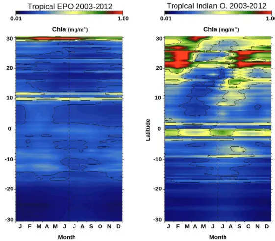
59 2.1 Hovmöller diagram of the sea surface chlorophyll-a for the Pacific Ocean (left) and the Indian

Ocean (Right) during the period 2003-2010……...

62 2.2 Hovmöller diagram of the sea surface temperature for the Pacific Ocean (left) and the Indian

Ocean (Right), during the period 2003-2010……...

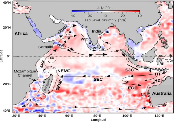
63 2.3 Indian Ocean study area. SLA fields during the South western monsoon season. Currents

vectors overlapped Great Whirl (GW), West Indian Coastal Current (WICC), South Monsoon

Current (SMC), Southern Gyre (SG). Northeast and Southeast Madagascar Current (NEMC,

SEMC), East African Coastal Current (EACC), Agulhas Current (AC), South Equatorial Current

(SEC), East Gyral Current (EGC), South Java Current (SJC), Halloway Current (HC), Indonesian

Throughflow (ITF) and Leeuwin Current (LC) (currents vectors taken from Schott, 2009 and Fieux,

2001)……...

64 2.4 Sea Leval Anomaly (SLA) topography in the EPO with principal currents overploted. California

current (CC), North Equatorial Current (NEC), North Equatorial Counter Current (NECC), Costa

Rica Coastal Current (CRCC), South Equatorial Current (SEC), Humboldt Current (HC). Costa

Rica Dome (CRD)…...

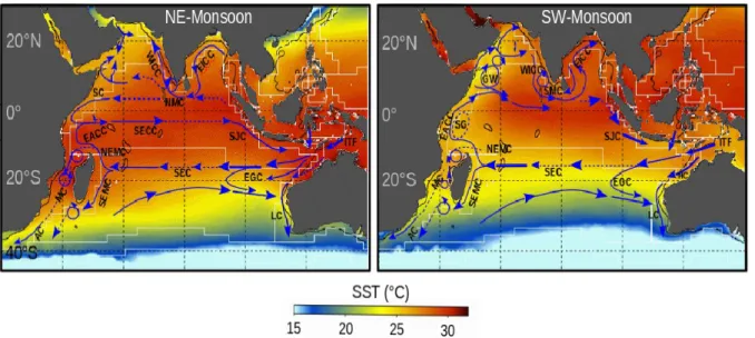
65 2.5 Indian Ocean sea surface temperature during the North Eastern Monsoon, December-Mars,

(left) and the South Western Monsoon, June-September, (right). Surface currents for each season

were overploted (blue arrows)...

66

(23)

2.6 Pacific Ocean sea surface temperature (°C) during March (left) and October (right) 2008...

...67

2.7 Annual mean thermocline depth (20°C isotherm depth) in the region of Costa Rica Dome. Data

from World Ocean Atlas 1998 (Conkright et al., 1999). (Taken from Fiedler, 2002)...

69 2.8 Sea surface temperature (left), sea surface chlorophyll (center) and eddy kinetic energy (right) in

the Pacific of Central America in February (average 2003-2012). CRD: Costa Rica Dome, PB:

Panama Bight...

70 2.9 Average chlorophyll concentration (2003-2012) in the Peruvian coastal upwelling in April,

during the maximum seasonal intensity of the upwelling.... …...

70 2.10 Mixed layer depth in (a) January and (b) July, based on a temperature difference of 0.2°C from

the near-surface temperature. Source From deBoyer Montégut et al. (2004). (c) Averaged maximum

mixed layer depth, using the 5 deepest mixed layers in 1° × 1° bins from the Argo profiling float

data set (2000–2009) and fitting the mixed layer structure as in Holte and Talley (2009)...

72 2.11 Oxygen concentration in the world oceans in micro-moles per liter. Nor the low values in the

north-western Indian Ocean and the Eastern Pacific Ocean (Taken from the World Ocean Review,

2010)...

73 2.12 Oxygen distribution (µM) at depth where oxygen concentration is minimal, indicating the

extend of the OMZ (red color) according to WOA205 climatology. Color bar corresponds to a 1 ± 2

µM interval between 0 and 20 µM, and a 20 ± 2 interval between 20 and 340 µM. The isolines

indicate the limit of the upper OMZ CORE depth in meters with a 100m contour interval. (Source

Paulmier and Ruiz-Pino, 2009). Note the important levels in the Indian ocean, Arabian sea (AS),

Bay of Bengal (BB) and the Pacific Ocean, Eastern SubTropical North Pacific (ESTNP), Eastern

Tropical North Pacific, Eastern South Pacific. Eaastern North Pacific (ENP)...

74 2.13 Oxygen distribution (µM at ± 2 intervals) at depth where oxygen concentration is minimal,

according to WOA205 climatology and the CRIO criterion (O2 < 20 µM in the CORE) applied in

(24)

spring (a), summer (b), fall (c) and winter (d). Note the important levels in the Indian ocean

Arabian sea (AS), Bay of Bengal (BB) and in the Pacific Ocean Eastern SubTropical North Pacific

(ESTNP), Eastern Tropical North Pacific, Eastern South Pacific. Eastern North Pacific (ENP).

(Source Paulmier and Ruiz-Pino, 2009)...

75 2.14 Time-mean eddy kinetic energy (cm

2

_/s

2

_{) calculated from drifters observations. Values are}

shown at 1 degree resolution (R. Lumpking, NOAA/AOML)...

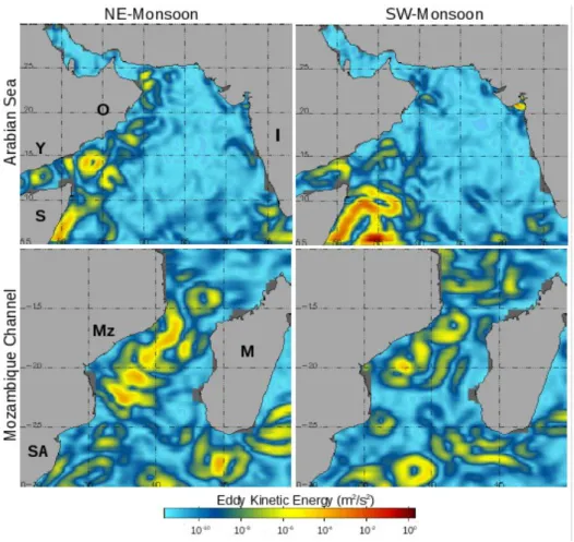
77 2.15 Eddy Kinetic Energy (EKE) in the Indian Ocean during the south-west monsoon. The

countries in the north-east of the basin are Oman (O) Yemen (Y), Somalia (S), India (I) and in the

south-east of the basin are Mozambique (Mz), South Africa (SA) and Madagascar (M)...

78 2.16 Eddy Kinetic Energy (EKE) in Central America during the month of march and the October

2010. The countries in the northern and southern Pacific Ocean's hemispheres are Mexico (M) with

the Gulf of Tehuantepec (G.T), Costa Rica (CR) with the Gulf of Papagayo (G.Pp) and Panama (P)

with the Gulf of Panama (G.P). Peru (Pr) and Chile (C)...

79 2.17 Indian Ocean Dipolo, positive phase (upper panel), negative phase (bottom panel) (taken from

E. Paul Oberlander, Woods Hole Oceanographic Institution)...

81 2.18 Schematic effect of “La Niña”, normal conditions and “Niño” events in the EPO, on the SST

and thermocline structure (Taken from NOAA TAO Diagrams)...

81 3.1 Purse seine activity (Source

http //www.wandering101photography.com

)...

84 3.2 Tuna purse seine vessel (left) (source FAO) and purse seine net (right) (source NOAA)...

84 3.3 3D diagram of a Payao anchored FAD (left) (source FAO), bamboo payao on the ocean surface

(right) (source ISSF)...

87

(25)

3.4 Drifting FAD with net, underwater view (left) and surface view (Source ISSF)...

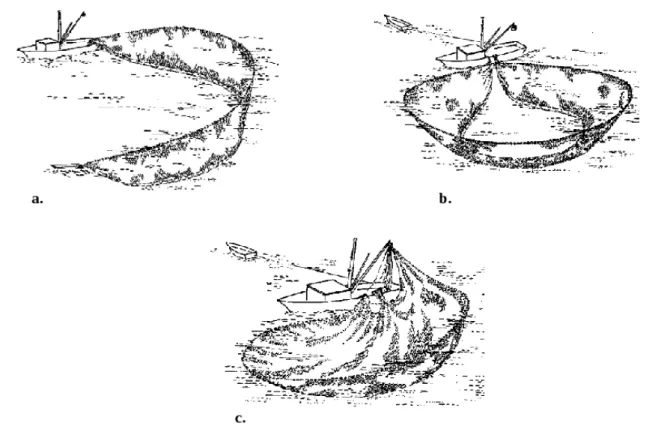
88 3.5 Tree main stages of purse seining operations, a. Setting the seine, b. Pursing the seine, c.

Hauling the seine. (Taken from Pravin, 2002)...

89 3.6 Tropical tuna principal morphological characteristics. a) Yellowfin tuna, common names:

Yellowfin tuna (USA), Albacore (France), Rabil (Spain) or Atun Aleta amarilla (LatinAmerica). b)

skipjack tuna, common names: Skipjack tuna (English), Listao (French), Listado, Barrilete

(Spanish) and c) bigeye tuna, common names: Bigeye tuna (English), Thon obèse/Patudo (French),

Patudo (Spanish)...

92 3.7 Global distribution of tropical tunas, a) Yellowfin tuna, b) skipjack tuna, c) bigeye tuna (Map

source:Majkowski, 2005; FAO, 2005)...

93 4.1 Latitudinal variability of tropical tuna catches in the Indian ocean (20°S to 13°N) across

Mozambique channel and Somalia regions for 4 temporal strata (quarters, plain lines) and climatic

seasons (dashed lines). Upper panel quarters 1 and 3 vs North-East Monsoon and South-West.

Lower panel quarters 2 and 4 vs both inter-monsoon seasons...

99 4.2 Average catch size in weight taken by the EU purse seine fishery in the Indian Ocean during

1990-2006 by species, yellowfin tuna (YFT) (left), bigeye tuna (BET) (right). (Taken from

Fonteneau, 2007)...…

100 4.3 Mean weight for the 3 species caught under FADs...

100 4.4 Idem as the previous figure for FS. Note the different scale...

101 4.5 Relative abundance of tropical tuna in the Indian Ocean during the period 2003-2010. Free

school (left) and FADs (right) from the SPECIES database...

102

(26)

4.6 Capture (metric tonnes) and Number of activities per year of the purse seine fishery in the

Indian Ocean from 2003 to 2010...

102 4.7 Location of catches on FS (blue circles) and FADS (red circles) for YFT (2003-2010)...

103 4.8 Location of catches on FS (blue circles) and FADS (red circles) for SKJ (2003-2010)...

103 4.9 Location of catches on FS (blue circles) and FADS (red circles) for BET (2003-2010) …...

103 4.10 Tuna presence (left) and absence (right) in the single catch sets during the 2003-2010. YFT

(orange), SKJ (Blue), BET (red). Catches for both fishing modes (Fee school and FADs) are

mixed...

104 4.11 El Niño anomalies during the period of study during 2007 and 2008, red color shows El Niño

events and blue La Niña events. Values 2008 indicate La Niña moderate event (Source

NOAA)...

105 4.12 Relative abundance of YFT (yellow color), SKJ (blue color) and BET (red color) caught on

free school(s), FADs and LOGs in the Eastern Pacific Ocean (EPO), during 2007 –

2008...

106 4.13 Relative sizes proportions (small, medium and large) for YFT in the EPO by set type/fishing

mode. Note that size ranges are different from those found for the Indian

Ocean...

107 4.14 Relative sizes proportions (small, medium and large) for SKJ in the EPO by set type/fishing

mode. Note that size ranges are different from those found for the Indian

Ocean...

107 4.15 Relative sizes proportions (small, medium and large) BET in the EPO by set type/fishing

mode. Note that size ranges are different from those found for the Indian

(27)

Ocean...

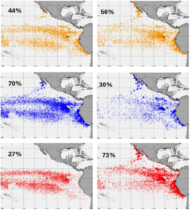
107 4.16 Tuna presence (left) and absence (right) in the single catch sets during the 2007-2008 period in

the EPO. YFT (orange), SKJ (Blue), BET (red). Catches for three sets types/fishing modes (School,

Logs and FADs) are mixed...

108

4.17 Relative match between catch locations (left) and the number observation from the

environmental parameter SST (right) in the EPO during July 2007...

109 4.18 Example of simultaneous data sets from MODIS during a 3-day period (SST, left and SSC,

center) and from SLA (right), 7-days corresponding average, showing eddies heights in the

Mozambique channel...

110 4.19 Example of eddy kinetic energy showing the Eastern Pacific Ocean (EPO) and the Indian

Ocean (IO) study areas...

111 4.20 Example of bathymetry for the Indian Ocean with ETOPO1 (logarithmic scale)...

111 4.21 Dynamics -historic behavior- of the chlorophyll-a concentration...

112 4.22 Quantification of the dynamic of the surface chlorophyll using an optimal interval of

variability, maximized from 3 to 12 days before the catch...

112 4.23 Example of the eddy borders computation in the EPO yellow circles show eddies. Distance to

eddy borders computation in km in the EPO...

113 4.24 Computation of distance to fronts (a) splitting fronts into weak and strong intensity (b)

computation of associated front probability (c) resulting distance (km). Example for the

IO...

114

(28)

4.25 Number of observations of single fishing sets...

115 4.26 Kernel density of the same catches, using a spatial radius of 100 km...

115 4.27 Result of partially spatial random positions, from left to right. Original positions, random with

a range of 50 km, 150 km and 250 km respectively...

115 5.1 Mean wind velocity (June) and surface currents related to the three study areas Morocco,

Mozambique Channel and north-western Australia. Atlantic Ocean currents Azores Current (AC),

Canary Current (CC), North Equatorial Current (NEC), North Equatorial Counter Current (NECC).

Indian Ocean currents Great Whirl (GW), West Indian Coastal Current (WICC), South Monsoon

Current (SMC), Southern Gyre (SG). Northeast and Southeast Madagascar Current (NEMC,

SEMC), East African Coastal Current (EACC), Agulhas Current (AC), South Equatorial Current

(SEC), East Gyral Current (EGC), South Java Current (SJC), Halloway Current (HC), Indonesian

Throughflow (ITF) and Leeuwin Current (LC)...

125 5.2 Effects of the preliminary smoothing of 4 km resolution SST data on the front detection. Weak

fronts are defined for the gradient interval 0.02-0.042 °C km

-1

_{(gray background) and strong fronts}

for gradients > 0.042 °C km

-1

_{. The data correspond to the average of five clear images for each of}

the three study areas, Morocco, Mozambique Channel and north-western Australia (i.e., totaling 15

images). (a-b) The total number of frontal pixels for the three detection window sizes, 32×32 (left

column), 24×24 (middle column) and 16×16 pixels (right column) and the three filters, Gaussian

(blue dashed line), median (red line) and average (green dashed line) applied at four kernel sizes,

3×3, 5×5, 7×7 and 9×9 pixels. Data for images where no smoothing was performed are labeled “no

conv.” (black dots). The “reference” or standard smoothing (3×3 median W32), generally used in

front detection, is represented by black squares. The red and green squares show the best

quantitative and visual results for both weak and strong fronts, obtained with median 7×7 and 5×5

respectively. The images show front detections for north-western Australia on November 24

th

_{, 2009}

for (c) 3×3, (d) 5×5, (e) 7×7 and (f) 9×9 pixel kernel sizes for the the median filter at window sizes

of W32 (left column), W24 (middle left column) and W16 (middle right column) and the average

filter at the W16 window size (right column). …...

130

(29)

(black dots) and for each combination of filter type (Gaussian, median and average), kernel (3×3,

5×5, 7×7 and 9×9 pixels) and window size (32×32, 24×24 and 16×16 pixels), as in Figure 2a and b.

…...

131 5.4 SST and associated fronts detected in November 24

th

_{2009 in north-western Australia at (a) 1}

km resolution with standard “reference” parameters (i.e., a median filter with a 3×3 pixel kernel and

a window size of 32×32 pixels); and (b) 4 km resolution with the optimal smoothing combination of

a median filter with kernel sizes of 5×5 and 7×7 for strong and weak fronts respectively, and

window size of 16×16...

132 5.5 (a-b) Improvement in the detection of thermal fronts between window sizes of 32x32 (left) and

16x16 pixels (right) in the Moroccan upwelling region in February (average 2003-2012) using the

optimal smoothing combination of a median filter, kernel sizes of 5×5 for strong fronts and 7×7 for

weak fronts. (c-d)The black rectangles highlight the areas where substantial improvements in front

detection using the 16x16 window size were observed over the shelf in a complex coastal

environment. The 200 m isobath is superimposed in the zoom frames (bottom)...

133 5.6 Histograms of the Sobel gradient associated to frontal pixels for the Moroccan region from daily

sea surface temperature (SST) data (2003-2012). (a) Sobel gradients for 1 km, 2 km and 4 km SST

data for 16x16 pixel window size, (b) SST gradient values normalized relative to the 4 km data

gradient scale and (c) SST gradient variability according to the size of the detection window, i.e.,

16×16, 24×24 and 32×32. The populations of frontal pixels associated to weak and strong gradients

in (b) and (c) are hatched and striped, respectively, while the left of the histograms indicates pixel

gradients that are below the 0.02 °C km

-1

_threshold...

₁₃₄

5.7 (a,b) Sea surface temperature (SST) gradient values used to validate (c-n) front detections

computed from smoothed SST data with a 5×5 median filter for strong fronts and a 7×7 median

filter for weak fronts for window sizes 32×32, 24×24 and 16×16 for the Moroccan region (c-h) and

north-western Australia (i-n). Percentages are expressed as the proportion of fronts detected

associated with both weak and strong gradients (in green) at a maximum distance of three pixels.

Frontal pixels that are not associated with an SST gradient are shown in red...

135

(30)

5.8 Application of the optimal smoothing combination (median filter, 5×5 kernel for strong fronts,

7×7 kernel for weak fronts, using a detection window of 16x16 pixels) for front detections on 10

years (2003-2012) of daily sea surface temperature (SST) data in the Indian Ocean during the

north-east monsoon (December to March) and the south-west monsoon (June to September). (a) Average

surface wind field for the same period (Cross-Calibrated Multi-Platform wind product; http

//podaac.jpl.nasa.gov/Cross-Calibrated_Multi-Platform_OceanSurfaceWindVectorAnalyses), (b)

SST with the main currents (current abbreviations as in Figure 1) and occurrence of thermal fronts

of (c) weak and (d) “strong” intensity. The Longhurst (2010) ecological provinces are

superimposed...

138 6.1 modeling scheme constructed to analyze the environment conditions for yellowfin tuna (YFT),

skipjack tuna (SKJ) and bigeye tuna (BET) fishing grounds, derive from single set tuna catch

records in the Indian Ocean. Catch models (green area), random models (gray area) and dominance

models (yellow area) show the model ID (1 to 16), the size of the species (small, large and the

unique size for SKJ) the fishing mode related (FS or FADs) and the total percentage of explanation

in parenthesis. For BRT general models (1 and 2) the percentage of contribution of the more

important predictor, size, is shown...

142 6.2 Boosted Regression Tree fitted function for yellowfin tuna (YFT) general model (1) with 72%

explained variance, red line shows the smooth function for continues variables (left). Relative

contributions of all predictors (right)...

148 6.3 Boosted Regression Tree fitted function for Skipjack tuna (SKJ) general model (2) with 74%

explained variance, red line shows the smooth function for continues variables (left). Relative

contributions of all predictors (right)...

148 6.4 Boosted Regression Tree fitted function for Bigeye tuna (BET) general model 3 with 74%

explained variance, red line shows the smooth function for continues variables (left). Relative

contributions of all predictors (right)...

149 6.5 Relative contribution of the variables for small-sized tunas catch on free school (left) (in

percentage). Net diagram of the contributions (right)... ...

150

(31)

6.6 BRT fitted function for small-sized yellowfin tuna (sYFT) on free school (FS)...

151 6.7 BRT fitted function for small-sized bigeye tuna (sBET) on free school (FS)...

151 6.8 Small bigeye tuna (sBET) catches on sea level anomaly (left), distance to anticyclonic (center)

and distance to cyclonic eddies (right) fields, during the south western monsoon (SW). Each star

plotted represent the locations of more than one set...

151 6.9 Relative contribution (in percentage) of the variables for large-sized tunas (left) on free school.

Net diagram of the contributions (right)...

152 6.10 BRT fitted function for large-sized yellowfin tuna on free school (FS)...

152 6.11 BRT fitted function for large-sized bigeye tuna on free school (FS). …...

152 6.12 Large-sized yellowfin tuna (lYFT) catches on sea level anomaly (left), distance to anticyclonic

(center) and distance to cyclonic eddies (right) fields, during the north eastern monsoon (NE). Each

star plotted represent the locations of more than one set. White stars shows high catches while blue

stars represent sets with lower catches...

152 6.13 Relative contribution (in percentage) of the variables for small-sized tunas (left) on FADs. Net

diagram of the contributions (right)...

154 6.14 BRT fitted function for small-sized yellowfin tuna on associated school (FADs)...

155 6.15 BRT fitted function for small-sized bigeye tuna on associated school (FAD)s...

155 6.16 Bathymetry, note 3000 m (light black line) and 4000 m (dark black line) contours. Bigeye tuna

catches overploted (red points)...

155 6.17 Relative contribution (in percentage) of the variables for large-sized tunas (left) on FADs. Net

diagram of the contributions (right)...

156

(32)

6.19 BRT fitted function for large-sized bigeye tuna on associated school (FAD)s...

157 6.20 Relative contribution (in percentage) of the variables for skipjack (left) on FADs. Net diagram

of the contributions compared with yellowfin and bigeye tuna small sizes (right)...

158 6.21 BRT fitted function for small-sized SKJ individuals caught on FADs...

158 6.22 BRT output (upper panel) and histogram the fishing grounds distribution for Chla, FADs are

shown in red and free school in blue (bottom panel) (see appendix C)...

159 6.23 Sea surface chlorophyll (left), note 0.2 and 0.4 (mg/m3) contour and thermal fronts (right) with

SKJ tuna catches overploted (white stars)...

159 6.24 BRT fitted function for small-sized YFT individuals caught on FS...

160 6.25 Boosted Regression Tree fitted function for Dominance, small sized individuals on FADs

model 13: sYFT (upper panel) and model 14: sBET (bottom panel)

...162

6.26 Boosted Regression Tree fitted function for Dominance models on FADs, large YFT and SKJ

(model 15, 38% and 16, 46%)...

163 6.27 Conceptual model of the relationships observed between Distance to eddies and Catch by

size...

165 6.28 EKE (left column) and Distance to eddies (right column) for small BET on FS (model 5,

upper row), for large BET on FS (model 9, middle row) and for large YFT on FADs (model 10,

lower row)...

166 6.29 Boosted Regression Tree fitted function for Random model 4.1 (28%)...

167 7.1 Yellowfin tuna fishing grounds respectively for school (blue), log (green) and fads (red) fishing

modes in the EPO...

170 7.2 Modeling scheme constructed to analyze the environment conditions for yellowfin tuna (YFT)

fishing grounds, derived from single set catch records in the Eastern Pacific Ocean. Catch models

(33)

(green area), random models (gray area) and dominance models (yellow area) with model ID (1 to

11), separated by size (small, medium and large) and then by fishing mode (FS, LOG and FADs).

The total percentage of explanation is given between parenthesis...

171 7.3 Boosted Regression Tree fitted function for yellowfin tuna (YFT) general model (1) with 41%

explained variance, red line shows the smooth function for continues variables (upper panel).

Relative contributions of all predictors (bottom panel). Note the similar relative importance of

several variables...

176 7.4 Boosted Regression Tree fitted function for small yellowfin tuna (YFT) caught on FS model 2

(upper panel) and for small YFT caught on FADs model 3 (bottom panel) with 37% and 18% of

explained variance respectively. Red line shows the smooth function for continues variables...

177 7.5 SST from model 3 with its distributions on YFT fishing grounds overploted (left). SSC from

model with its distribution on the fishing grounds overploted. Note the positive relationship

between catch and the conditions imposed by FADs, specially the low level of pigment

concentration. (See appendix D, fishing grounds for SST and SSC)...

176 7.6 Small-sized YFT caught on FS, blue, (left) and caught on FADs, red, (right) over SSC field for

2007... ..

178 7.7 Boosted Regression Tree fitted function for medium yellowfin tuna (YFT) caught on LOG

model 4 with 40% of explained variance. Red line shows the smooth function for continues

variables...

179 7.8 YFT medium-sized catches (withe circles) over strong frontal occurrence field for 2007(left)

and zoom of the Costa Rica Dome area (right) . Note how catches on this area are mainly located at

distance >400 km from the strong coastal fronts. This pattern is different to what is observed in the

Peru-upwelling area where catch are located close to the coast...

179 7.9 Boosted Regression Tree fitted function for medium yellowfin tuna (YFT) caught on LOG

model 5 with 33% of explained variance. Red line shows the smooth function for continues

variables...

180

(34)

7.10 Barplot of relative contributions for medium yellowfin tuna (YFT) caught on FADs model 6

with 20% of explained variance...

180 7.11 Boosted Regression Tree fitted function for large yellowfin tuna (YFT) caught on FS model 7

with 39% of explained variance and relative contributions in percentage. Red line shows the smooth

function for continues variables...

181 7.12 Comparison between large-sizes YFT catch levels on FS (discontinuous line) and

environmental conditions of the YFT FS fishing grounds, in density, for SST (left) and SSC (right).

(See appendix D, fishing grounds histograms for SST and SSC)...

181 7.13 Boosted Regression Tree fitted function for large yellowfin tuna (YFT) caught on FADs model

8 with 35% of explained variance and relative contributions in percentage. Red line shows the

smooth function for continues variables...

182 7.14 Comparison between large-sizes YFT catch levels on FADs (discontinuous line) and

environmental conditions of the YFT FADs fishing grounds, in density, for SST (left) and SSC

(right). (See appendix D)...

182 7.15 Large-sized YFT caught on FS, blue, (left) and caught on FADs, red, (right) over SSC field for

2007...

183 7.16 Boosted Regression Tree fitted function for medium-sized yellowfin tuna (YFT) caught on FS

model 4.1 with 31% (upper panel) and caught on LOG model, 5.1 30% of explained variance

(bottom panel) . Red line shows the smooth function for continues variables...

.

184 7.17 Boosted Regression Tree fitted function for medium-sized yellowfin tuna (YFT) caught on FS

model 11 with 41% of total explained variance. Red line shows the smooth function for continues

variables...

185 8.1 Chapters of the thesis work...

189

(35)

8.3 SST from model 3 with its distributions on YFT fishing grounds overploted (left). SSC from

model with its distribution on the fishing grounds overploted. Note the positive relationship

between catch and the conditions imposed by FADs, specially the low level of pigment

concentration(same Figure 7.5 in Chapter 7 )...

192 8.4 Deployment and sets positions (courtesy Dr. Martin Hall, IATTC)...

192 8.5 Scheme of work already done (yellow) and the future work propose (green) to determine the

ecological effects of FADs...

193 A1 Monthly variation of the Indian Ocean water pool, from January to June. Contour shows sea

surface temperature of 28°C...

214 A2 Monthly variation of the Indian Ocean water pool, from July to December. Contour shows sea

surface temperature of 28°C...

215 B.1 Presence/Absence (left, right respectively) of tropical tuna on free school in the Indian Ocean

during 2003-2010. Yellowfin tuna (upper panel), skipjack (center panel), bigeye (bottom

panel)...

217 B.2 Presence/Absence (left, right respectively) of tropical tuna on FADs in the Indian Ocean during

2003-2010. Yellowfin tuna (upper panel), skipjack (center panel), bigeye (bottom panel)...

218 B.3 Presence/Absence (left, right respectively) of tropical tuna on Free School in the EPO during

2007-2008. Yellowfin tuna (upper panel, orange), skipjack (center panel, blue), bigeye (bottom

panel,red)...

219 B.4 Presence/Absence (left, right respectively) of tropical tuna on FADs in the EPO during

2007-2008. Yellowfin tuna (upper panel, orange), skipjack (center panel, blue), bigeye (bottom

panel,red)...

220 B.5 Presence/Absence (left, right respectively) of tropical tuna on LOGs in the EPO during

2007-2008. Yellowfin tuna (upper panel, orange), skipjack (center panel, blue), bigeye (bottom panel,red)

…...

221

Mesoscale structure and dynamics of the tropical tuna's associated-environment in the Indian and the Eastern Pacific Oceans : comparative approach

HAL Id: tel-03217624

https://tel.archives-ouvertes.fr/tel-03217624

Mesoscale structure and dynamics of the tropical tuna’s

associated-environment in the Indian and the Eastern

Pacific Oceans : comparative approach

Carmen Liliana Roa Pascuali

To cite this version:

Mesoscale structure and dynamics of the

tropical tuna’s associated-environment in the

Indian and the Eastern Pacific Oceans;

comparative approach

Structure de méso-échelle et dynamique de

l'environnement des thonidés tropicaux dans

l’Océan Indien et l’Océan Pacifique Est ;

approche comparative

Délivré par l’Université de Montpellier

Préparée au sein de l’école doctorale SIBAGHE

Et de l’unité de recherche MARBEC

(IRD / IFREMER /

Université de Montpellier / CNRS)

Spécialité : ÉCOSYSTÈMES

Présentée par Carmen Liliana ROA PASCUALI

Soutenue le 15 janvier 2016 devant le jury composé de

To my family,

To my daughter Manuela "tuti"

who came to my life to teach me what is the true love about.

Abstract

Résumé

Acknowledgments

“We don't meet people by accident. They are meant to cross our path for a reason”

(Unknown)

A

Agradecimientos

“No conocemos a las personas por accidente, ellas se cruzan en nuestro camino por una razón”

(Anonimo).

E

Contents

Résumé Exécutif

...

41

1 Introduction

...

54

2 Indian Ocean and Eastern Pacific Ocean: general oceanographic characteristics

...

61

2.1 Large scale comparison between Indian Ocean and Eastern Pacific Ocean...

61

2.1.1 Indian Ocean...

63

2.1.2 Eastern Pacific Ocean...

64

2.2 Oceanographic characteristics...

65

2.2.1 Sea Surface temperature (SST)...

65

2.2.2 Sea surface chlorophyll (SSC)...

68

2.2.3 Mixed Layer Depth (MLD)...

71

2.2.4 Dissolved Oxygen...

73

2.2.5 Eddy Kinetic energy (EKE)...

76

2.2.6 Particularities of the current patterns in the Indian Ocean...

79

2.2.7 Indian Ocean Dipole...

80

2.2.8 El Niño and La Niña conditions...

80

3 Purse seine fisheries and tropical tuna species

...

83

3.1 Purse-seine Fisheries...

83

3.1.1 Set types...

85

3.1.1.1 Free school sets...

85