HAL Id: tel-03213278
https://tel.archives-ouvertes.fr/tel-03213278
Submitted on 30 Apr 2021
HAL is a multi-disciplinary open access archive for the deposit and dissemination of sci-entific research documents, whether they are pub-lished or not. The documents may come from teaching and research institutions in France or
L’archive ouverte pluridisciplinaire HAL, est destinée au dépôt et à la diffusion de documents scientifiques de niveau recherche, publiés ou non, émanant des établissements d’enseignement et de recherche français ou étrangers, des laboratoires
Iris-Amata Dion
To cite this version:
Iris-Amata Dion. Ice injected up to the tropical tropopause layer by deep convection. Meteorology. Université Paul Sabatier - Toulouse III, 2019. English. �NNT : 2019TOU30320�. �tel-03213278�
THÈSE
THÈSE
En vue de l’obtention du
DOCTORAT DE L’UNIVERSITÉ DE TOULOUSE
Délivré par : l’Université Toulouse 3 Paul Sabatier (UT3 Paul Sabatier)
Présentée et soutenue le 25 Octobre 2019 par :
Dion Iris-Amata
Glace injectée dans la Tropopause Tropicale par Convection Profonde
JURY
ATTIE JEAN-LUC Professeur d’Université Président du Jury
CLAUD CHANTAL Directrice de Recherche Rapporteure
SANTEE MICHELLE Directrice de Recherche Rapporteure
RICAUD PHILIPPE Directeur de Recherche Directeur de Thèse
HAYNES PETER Professeur Directeur de Thèse
CARMINATI FABIEN Ingénieur de Recherche Examinateur
RIVIERE EMMANUEL Maître de Conférences Examinateur
École doctorale et spécialité :
SDU2E : Océan, Atmosphère, Climat Unité de Recherche :
Centre National de Recherches Météorologiques (CNRM), Météo-France – CNRS (UMR 3589)
Directeur de Thèse :
RICAUD Philippe, HAYNES Peter Rapporteur :
Ice injected up to the Tropical Tropopause Layer
by Deep Convection
Author: Iris-Amata DION Thesis supervisor: Philippe RICAUD Co-supervisor of the thesis: Peter HAYNES Thesis of the Toulouse III University - Paul Sabatier Defended 25/10/2019 at Météo-france, Toulouse, France
À mon grand frère, mon inspiration !
À mes parents, ces aventuriers, qui m’ont toujours écoutée et encouragée à faire ce qui m’inspire.
À Gaël, pour tant et pour tout.
« Ooh mais elle est Trop-po-pausée cette thèse ! », « Une thèse sur la glace ? Tu veux dire, sur la glace à la vanille, à la framboise ou au chocolat? » Quelques perles entendues.
A l’issue de la rédaction de ce manuscrit, j’aimerais exprimer ma gratitude envers toutes celles et ceux qui m’ont accompagnée, conseillée, écoutée, encouragée et soutenue durant ma thèse. Merci à vous.
Mes directeurs de thèse et l’équipe TEASAO. Merci à Philippe et Peter,
pour m’avoir accueillie et fait confiance dans l’élaboration de cette thèse. Ce fut pour moi une expérience enrichissante. J’ai pu découvrir différentes facettes du monde de la recherche, aussi bien les opportunités que les difficultés. Plus parti-culièrement, merci Philippe pour m’avoir donné la possibilité de participer à des conférences et à une école d’été. Ce furent des voyages très enrichissant. Merci aussi pour les nombreuses relectures de mes travaux. Peter, merci beaucoup pour ton accueil à Cambridge ! J’en garde un excellent souvenir. Merci aussi à l’équipe TEASAO pour m’avoir permis de faire cette thèse et pour m’avoir accompagnée tout au long de celle-ci.
Les membres du jury,Michelle Santee, Chantal Claud, Fabien Carminati,
Emmanuel Rivière, Yves Morel et Jean-Luc Attié. Merci d’avoir accepté de lire et d’échanger autour de mes travaux. I would especially like to thank Michelle for her many and helpful feedback.
Claire Doubremelle. Sincèrement merci pour votre soutien et votre écoute et pour avoir su adoucir certaines situations avec beaucoup d’empathie.
L’équipe COMETS et en particulier Béatrice Josse., Virginie Marécal. et Sophie Belamari., merci pour vos conseils, votre bienveillance, et votre soutien. Merci d’être régulièrement venues me rappeler votre présence en cas de doutes. Béa, merci de m’avoir consacré du temps avec beaucoup de douceur lors des mo-ments plus difficiles. Merci beaucoup aussi pour tes conseils sur mes travaux
et sur les différents jeux de données pouvant être intéressants! Virginie, merci beaucoup d’avoir relu une partie de mes travaux et merci beaucoup pour tes
en-couragements! Laaziz El Amraoui., merci d’avoir veillé au bon déroulement de
ma thèse et d’avoir été membre de mon comité de thèse.
Jean-Pierre Chaboureau, merci pour m’avoir fourni des données du modèle Meso-NH et merci pour ta confiance.
Fabien Carminati, merci pour tes retours enrichissants sur mes travaux. Merci aussi pour l’agréable accueil à Exeter et pour avoir organisé à mon inten-tion ce séminaire, qui, au cours de ma deuxième année de thèse, m’a fait gagner confiance en moi et en mes travaux!
Thibaut Dauhut, un grand merci pour tes conseils dès le début de ma thèse et tout au long de celle-ci. Merci pour ton écoute, tes explications et pour nos discussions sur les divers processus dans la tropopause tropicale, tout en traversant King’s College! Tu as été un modèle (sans jeu de mot ..) et un ami.
Samuel Q., Valentin P. et Cyrille D., un grand merci pour m’avoir consacré du temps et de l’énergie dans l’apprentissage d’un nouveau langage informatique. Merci aussi à toutes les très chouettes personnes rencontrées lors de
con-férences et durant l’école d’été à Cape Town. Je pense notamment à Suneeth
K V et Moha Diallo mais aussi à bien d’autres.
Les amies du CNRM, dans le désordre, merci à vous: Maxence De-scheemaecker, mon co-bureau, merci pour avoir été toi-même, drôle, touchant
et enthousiaste. Une bienveillance "co-bureautale" plus qu’apréciée ! Damien
Specq, merci pour ton amitié, les chouettes moments partagés et ces joies de
nous voir progresser aux cours d”équi"! Yann Cohen, merci pour ton écoute, ton
ont obligés à faire des pauses.Matteo Ponzano, Thomas Drugé et Léo Ducongé,
merci pour votre jolie cohésion très vivante. Quentin Fumiere, merci pour avoir
partagé ces années de thèse dans une atmosphère humoristique bien à toi :-)César
Sauvage, merci pour ces moments de guitare, saxo et chant. Hugo Marchal,
merci pour m’avoir laissée gagner au ping-pong! Yannick et Nizar, merci pour
vos encouragements, et vos longs débats avec Maxence. Valentin Petiot merci
pour nos partages et pour nos découvertes de toutes sortes de thés lors de
discus-sions sur les Pyrénées. Merci pour ton amitié. Guillaume Bigeard Kurt, merci
pour tes conseils de post-doc, les couchers de soleil sur les Pyrénées depuis le
CNRM et tout plein d’autres moments très sympas. Gab Lellouche, merci pour
ta super belle énergie!P-A J., merci pour tes partages de musique qui ont
accom-pagné certains moments de ma thèse. Marie Mazoyer, un très grand merci pour
ce coup de pouce, ce "boost" de confiance en soi, que tu m’as offert juste avant
ma soutenance !! Alexane Lovat, pour ton rire qui se propage si vite! Sabine
Radanovics, pour le chant et tes encouragements de dernière minute qui m’ont été si précieux !! merci aux joueurs de ping-pong de 13h00, et à tant d’autres, Claire Lamotte, Zied Sassi, Nicolas Maury, la chorale, le tissu aérien, la capoera, ...
Mes colocs, qui ont accompagné cette thèse avec du soleil: Étienne qui m’a inspirée et impressionnée par son énergie, sa vitalité et sa grande curiosité. Merci
pour ces énormes fêtes que tu sais incroyablement préparer. Brice qui m’a fait
rêver, chanter et danser. Hugo, qui a été et est toujours un bijou de sagesse et
d’amour, merci pour cela. Des amitiés précieuses.
ton fort soutien, tes conseils de doctorante, pour ta Folie qui éveille, élève et émerveille. Merci d’être une Perle précieuse de bonheur.
Merci aux pétillantescopines de Paris, Fleur, Alice, Rim et Mathilde! Merci
d’être venues me voir sur Toulouse. Vos fascinants projets, débordant d’aventure, m’ont inspirée et permis de prendre un dernier bol d’air chaud et doux avant la grande ligne droite de la fin de thèse. J’aimerais en profiter pour remercier plus
spécifiquement ma grande AmieMathilde : savions-nous déjà au lycée que nous
serions toujours toutes les deux étudiantes plus de 10 ans plus tard ? Merci pour ta bienveillance, tous tes encouragements, pour avoir toujours cru en moi, pour ta complicité, et ton amitié !
Merci àtoute ma famille. Merci Paulette pour tes encouragements. Merci à
ma grand mère, qui du haut de ses 92 ans, m’a toujours félicitée et encouragée!
Et bien sûr, par dessus tout, merci àmes parents et à Camille, merci pour tout !
Merci beaucoup aussi à tous les amis et la famille qui sont, pour certains, venus
de loin assister à ma soutenance : Séverine, Jean-Marc et Valérie, Pierre et
Louise, Mathilde, Fleur, Alice, Faustine, Marion et Jérémie! Séverine, merci aussi pour la relecture de dernière minute très précieuse !
Enfin et surtout,Gaël, merci d’être présent et de rayonner à mes côtés depuis le
début de nos années d’études. Merci d’avoir nourri de nombreux rêves et d’avoir partagé cette curiosité et cette sensibilité au vaste domaine des sciences de la Terre et de l’Univers. Tout cela nous a transportés depuis les roches terrestres jusqu’à, pour ma part, la Tropopause et toi, toujours plus haut, jusqu’à la planète Mars! Toute ma tendresse et ma reconnaissance pour le soutien et l’aide que tu m’as apportés, pour m’avoir relue plusieurs fois, conseillée, écoutée et finalement pour avoir grandement partagé cette aventure! Merci pour tout.
Abstract
Key words: Tropical Tropopause Layer, Maritime Continent, upper tropo-sphere, lower stratotropo-sphere, ice, precipitation, flashes, water vapour, MJO, ENSO, MLS, TRMM
The tropical tropopause layer (TTL) defined by the layer surrounding the cold point, delimiting the troposphere to the stratosphere, controls the vertical distri-bution of temperature, clouds, water vapour and ice. However, water vapour and cirrus clouds (clouds composed of ice) have a significant radiative effect on cli-mate. Furthermore, the way in which water vapour and ice are transported up to the TTL and even higher into the lower stratosphere is still not well understood. Among the main processes identified to control the humidity of the TTL, this the-sis focuses on the rapid (diurnal-scale) deep convective processes to estimate its impact on the amount of ice injected (∆IWC) into the TTL.
The Microwave Limb Sounder (MLS) instrument on board the Aura satellite have measured the ice water content (IWC) and water vapour mixing ratio in the upper tropophere (at 146 hPa) and near the cold point of the TTL (at 100 hPa) from 2004 to 2017 with measurements at a low temporal resolution of two local times per day: at 01:30 and 13:30 local times in the tropics. Instruments on-board the Tropical Rainfall Measuring Mission (TRMM) satellite have measured pre-cipitation (Prec) and number of flashes during thunderstorm events (Flash) from 2004 to 2015 in the tropics, with a much better temporal resolution than MLS allowing to study diurnal cycles with a 1-hour temporal resolution and a
horizon-tal resolution of 2◦ × 2◦ (∼ 200 × 200 km). Our studies focus on the austral
convective season of December, January and February (DJF).
Submillimeter-Wave Limb-Emission Sounder (SMILES) space-borne instrument, which was able to provide IWC in the TTL with a 1-hour temporal resolution from December 2009 to February 2010. ∆IWC in the TTL has been estimated over sev-eral oceanic and continental regions of the tropics (South America, South Africa, Indian Ocean, Pacific Ocean and Maritime Continent (MariCont, including In-donesia)), highlighting the highest values of ∆IWC over the MariCont. ∆IWC estimated from Flash and Prec have been compared to ∆IWC calculated from IWC provided by ERA5 meteorological reanalyses averaged from 2005 to 2016, over the MariCont. Over land, ∆IWC calculated from the different datasets (found
from 4 to 10 and from 0.5 to 3.5 mg m-3 at 146 and 100 hPa, respectively) are
larger than over sea (found from 0.2 to 4.0 and from 0.0 to 0.7 mg m-3at 146 and
100 hPa, respectively). The Java island, composed of high mountains (> 2000 m) abruptly reaching the sea, reveals the largest ∆IWC whatever of the dataset used
(∼ 1.5 and ∼ 8.5 mg m-3at 146 and 100 hPa, respectively). Finally, the impact of
large-scale intra-seasonal oscillations (Madden-Julian Oscillation (MJO) and La Niña) on ∆IWC in the TTL over the MariCont has been studied. During La Niña,
∆IWC tends to increase over land (from ∼ +4 mg m-3per pixel) and to decrease
over the sea (from ∼ -4 mg m-3per pixel) compared to ∆IWC estimated during
DJF. During the active phase of the MJO, small differences (< 1 mg m-3per pixel)
in ∆IWC are observed compared to ∆IWC obtained in DJF. The impact of the MJO in active and suppressed phases on ∆IWC are studied using ice provided by the meso-scale model Meso-NH. A complementary study has been drawn, apply-ing the model proposed in this thesis to the Asian monsoon area, known for its strong transport of air masses up to the stratosphere.
Résumé
Mots clés : Tropopause tropicale, teneur en eau glacée, Continent Mar-itime, précipitation, nombre d’éclairs, haute troposphère, basse stratosphère, vapeur d’eau, MJO, ENSO, MLS, TRMM.
La tropopause tropicale (TTL), définie par la couche autour du point froid, délimitant la troposphère de la stratosphère, contrôle la distribution verticale de la température, des nuages, de la vapeur d’eau et de la glace. Or la vapeur d’eau ainsi que les cirrus (nuages composés de glace) ont un effet radiatif important sur le cli-mat. Cependant, la façon dont la vapeur d’eau et la glace sont transportées jusqu’à la TTL et même au-delà jusqu’à la stratosphère est encore mal connue. Parmi les processus majeurs identifiés pour contrôler l’humidité de la TTL, cette thèse se focalise sur les processus rapides (à l’échelle diurne) de convection profonde dans le but d’estimer les quantités de glace injectées (∆IWC) dans la TTL.
L’instrument MLS (Microwave Limb Sounder) à bord du satellite Aura a mesuré la teneur en eau glacée (IWC) et le rapport de mélange en vapeur d’eau dans la haute troposphère (146 hPa) et proche du point froid de la TTL (100 hPa), de 2004 à 2017 mais avec des mesures à faible résolution temporelle de deux heures locales par jour : à 01h30 et 13h30 en heures locales dans les tropiques. Les instruments du satellite TRMM (Tropical Rainfall Measuring Mission) ont mesuré les précipitations (Prec) et le nombre d’éclairs lors d’évènements orageux (Flash) dans les tropiques de 2004 à 2015 avec une bien meilleure résolution tem-porelle que MLS permettant d’établir le cycle diurne avec une résolution d’une
heure et une résolution horizontale de 2◦×2◦ (∼ 200 × 200 km). Nos études se
focalisent sur la saison convective australe de décembre, janvier et février (DJF). La thèse propose un modèle reliant les observations de Prec et de Flash de TRMM, utilisées comme approximation de la convection profonde, et les deux
Submillimeter-Wave Limb-Emission Sounder), capable de fournir IWC dans la TTL avec une résolution temporelle d’une heure de décembre 2009 à février 2010.
∆IWC a été estimé sur plusieurs régions océaniques et continentales des tropiques
(Amérique du Sud, Afrique du Sud, Océan Pacifique, Océan Indien et le Conti-nent Maritime (MariCont, incluant l’Indonésie)), montrant les plus fortes valeurs de ∆IWC dans la TTL au-dessus du MariCont. Sur le MariCont, ∆IWC estimé à partir de Flash et Prec ont été comparés à ∆IWC estimé à partir des données de IWC fournis par les réanalyses météorologiques de ERA5 moyennées de 2005 à 2016. Sur les terres, ∆IWC calculés à partir des différents ensembles de données
(trouvé de 4 à 10 et de 0,5 à 3,5 mg m-3respectivement à 146 et 100 hPa) sont
plus grands que sur les mers (de 0,2 à 4,0 et de 0,0 à 0,7 mg m-3respectivement
à 146 et 100 hPa). L’île de Java, composée de hauts reliefs (> 2000 m) se jetant dans la mer, révèle les plus importantes valeurs de ∆IWC quel que soit le jeu de
données utilisé (∼ 8.5 et ∼ 1.5 mg m-3 respectivement à 146 et 100 hPa).
En-fin, l’impact des oscillations intra-saisonnières à grande échelle (Madden Julian Oscillation (oscillation de Madden-Julian (MJO) et La Niña) sur ∆IWC dans la TTL a été étudié sur le MariCont. Durant La Niña, ∆IWC tend à augmenter sur
les terres (de ∼ + 4 mg m-3par pixel) et diminuer sur les mers (de ∼ - 4 mg m-3
par pixel) par rapport à ∆IWC estimé durant DJF. Pendant la phase active de la
MJO, de faibles différences (< 1 mg m-3par pixel) de ∆IWC sont observées par
rapport à ∆IWC obtenu en DJF. L’impact de la MJO en phases actives et inhibées sur ∆IWC est étudié en utilisant la glace fournie par le modèle de méso-échelle Meso-NH. Une étude complémentaire a été réalisée, appliquant le modèle pro-posé dans cette thèse à la région de la mousson asiatique, connue pour son fort transport des masses d’air jusqu’à la stratosphère.
Contents
Remerciements . . . 5 Abstract . . . iii Résumé . . . v Mains acronyms . . . xv 1 Introduction 1 1.1 Introduction (English) . . . 1 1.2 Introduction (Français) . . . 12 Fundamentals in atmospheric physics and chemistry 11 2.1 Structure of the atmosphere and tropopause definitions . . . 11
2.1.1 Global atmospheric structure . . . 11
2.1.2 Tropopause, a level: thermal and dynamical definitions . . 12
2.1.3 Tropical Tropopause, a transition layer: the TTL . . . 16
2.2 Tropical convective structures and mechanisms . . . 18
2.2.1 Deep convective structures, diurnal variability and mech-anisms . . . 19
2.2.2 Diabatic processes . . . 22
2.2.2.1 Theoretical model of the air parcel . . . 23
2.2.2.2 Convective initiators and ascending processes . 23 2.2.2.3 Radiative processes . . . 25
2.2.2.4 Microphysical processes . . . 27
2.2.2.5 Turbulent processes . . . 28
2.2.2.6 Overshoots . . . 28
2.2.2.7 Subsidence, precipitation and cold pockets . . . 29
2.2.3 Geographical and seasonal variability of deep convection . 31 2.3 Tropical tropospheric and stratospheric dynamic processes . . . . 32
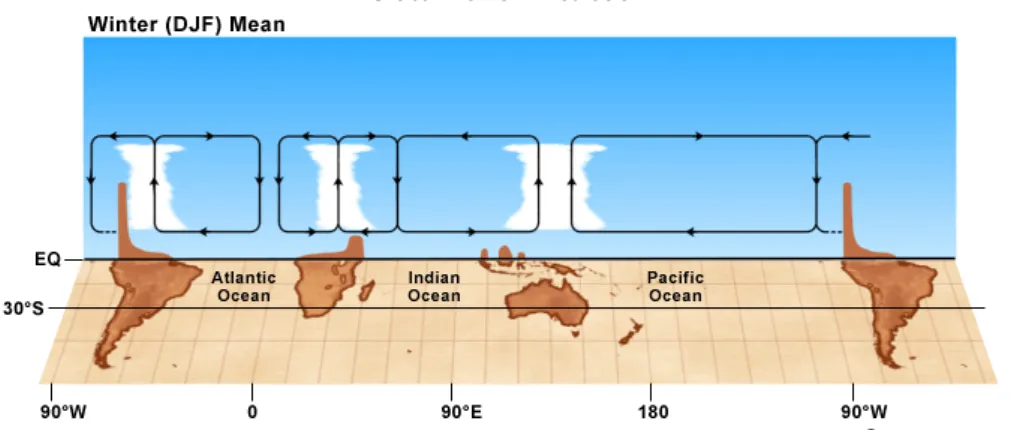
2.3.1 Tropospheric zonal transport of energy: the Walker cells . 32 2.3.2 Tropospheric meridional transport of energy : the Hadley circulation . . . 33
2.3.3 Tropical stratospheric dynamics: the Brewer and Dobson cirulation . . . 35
2.3.4 Equatorial Waves . . . 36
2.3.5 Times scales in the tropics: annual and diurnal cycles . . . 36
2.3.6 Madden Julian Oscillation . . . 39
2.3.7 El Nino Southern Oscillation . . . 42
2.3.8 Transport across the tropopause . . . 43
2.4 Water Budget in the tropics: Troposphere to Stratosphere . . . 46
2.4.1 Water Vapour and Ice . . . 46
2.4.2 Water Saturation and Relative Humidity . . . 48
2.4.3 Tropospheric Water Budget in the tropics . . . 49
2.4.4 TTL Water Budget . . . 50
2.4.5 Stratospheric water budget in the tropics . . . 52
2.5 Atmospheric characteristics over the Maritime Continent . . . 54
2.5.1 Precipitations over the MariCont . . . 55
2.5.2 Troposphere and stratosphere air masses exchanges over the MariCont and "Stratospheric fountain" . . . 56
CONTENTS
3 Instruments and models used 59
3.1 Satellite remote sensing observations: definitions and motivations 59
3.1.1 Orbital and viewing modes . . . 59
3.1.2 Overview of the satellites measuring Water vapour in the UTLS . . . 63
3.1.3 Overview of satellites measuring the Ice Water Content in the UTLS . . . 65
3.2 Instruments used . . . 66
3.2.1 MLS . . . 66
3.2.1.1 MLS instrument on the Aura platform . . . 66
3.2.1.2 MLS components characteristics . . . 67
3.2.1.3 WV and IWC diurnal cycles from MLS in trop-ics: the Day-Night method . . . 71
3.2.2 SMILES . . . 73
3.2.3 TRMM . . . 74
3.2.3.1 Deep convection estimation from TRMM . . . . 76
3.2.3.2 TRMM - 3B42 . . . 77
3.2.3.3 TRMM - LIS . . . 78
3.3 Meso-scale models and meteorological reanalysis used . . . 80
3.3.1 ERA5 . . . 81
3.3.2 Meso-NH . . . 81
3.3.3 NCEP/NCAR Reanalysis . . . 83
3.4 Chapter summary . . . 84
4 Ice injected into the TTL in the austral tropics 87 4.1 Article-1: Ice injected into the tropopause by deep convection – Part 1: In the austral convection tropics . . . 88
4.3 Chapter summary . . . 110
5 Ice injected into the TTL over the Maritime Continent 113 5.1 Article-2: Ice injected into the tropopause by deep convection – Part 2: Over the Maritime Continent . . . 114
5.2 Abstract . . . 114
5.3 Introduction . . . 115
5.4 Datasets . . . 119
5.4.1 MLS Ice Water Content . . . 119
5.4.2 TRMM-3B42 Precipitation . . . 120
5.4.3 TRMM-LIS number of Flashes . . . 121
5.4.4 ERA5 Ice Water Content . . . 122
5.5 Methodology . . . 124
5.6 Horizontal distribution of ∆IWC estimated from Prec over the MariCont . . . 125
5.6.1 Prec from TRMM related to IWC from MLS . . . 125
5.6.2 Convective processes compared to IWC measurements . . 128
5.6.3 Horizontal distribution of ice injected into the UT and TL estimated from Prec . . . 130
5.7 Relationship between diurnal cycle of Prec and Flash over Mari-Cont land and sea . . . 134
5.7.1 Flash distribution over the MariCont . . . 134
5.7.2 Prec and Flash diurnal cycles over the MariCont . . . 135
5.7.3 Prec and Flash diurnal cycles and small-scale processes . . 139
5.8 Horizontal distribution of IWC from ERA5 reanalyses . . . 143
5.9 Ice injected over a selection of island and sea areas . . . 146
5.9.1 ∆IWC deduced from observations . . . 146
CONTENTS
5.9.3 Synthesis . . . 150
5.10 Discussion on small-scale convective processes impacting ∆IWC over a selection of areas . . . 151
5.10.1 Java island, Sulawesi and New Guinea . . . 151
5.10.2 West Sumatra Sea . . . 152
5.10.3 North Australia Sea and seas with nearby islands . . . 153
5.11 Conclusions . . . 154
5.12 Author contribution. . . 157
5.13 Acknowledgement. . . 157
5.14 Data availability. . . 158
6 Impact of large-scale oscillations on the ice injected in the TTL over the Maritime Continent 159 6.1 Context . . . 159
6.2 Datasets, study zones and methodology . . . 161
6.2.1 Datasets . . . 161
6.2.2 Study zones . . . 162
6.2.3 Methodology . . . 162
6.3 Diurnal cycle of Prec over the Maritime Continent: comparison between the study periods . . . 166
6.4 Horizontal distribution of Prec and IWCM LS measured at 01:30 LT and 13:30 LT . . . 168
6.4.1 Prec during the increasing phase of the convection . . . . 169
6.4.2 IWCM LS in the UT during the increasing phase of the convection . . . 170
6.5 ∆IWC injected in the UT duringDJF, MJO active in MariCont andLa Niña . . . 172
6.5.2 ∆IWC duringMJO over island and sea of the MariCont . 175
6.5.3 ∆IWCP recduring the study periods over island and sea of
the MariCont . . . 177
6.6 Synthesis and discussion . . . 179
6.7 Acknowledgement . . . 181
7 Further works: Application of the methodology to the Asian monsoon region 183 7.1 Introduction . . . 184
7.2 Instruments and methodology . . . 185
7.3 Horizontal distributions of Prec, Flash and IWC over Asia . . . . 185
7.3.1 Horizontal distributions . . . 185
7.4 Diurnal cycle of Prec and Flash over the Asian study zones . . . . 189
7.5 Diurnal cycle of IWC over the Asian study zones . . . 191
7.6 Horizontal distribution of ∆IWC over Asia . . . 194
7.7 ∆IWC over Asian study zones . . . 195
7.8 Synthesis . . . 196
7.9 Author contribution. . . 198
8 Conclusions and perspectives 199 8.1 Conclusions (English) . . . 199
8.1.1 Issues and motivations: the TTL a transition layer be-tween the troposphere and the stratosphere . . . 199
8.1.2 Objectives and strategy . . . 200
8.1.3 Method used . . . 201
8.1.4 Validation . . . 202
8.1.5 Main results of the thesis . . . 203
CONTENTS 8.2.1 Tropical deep convection from space-borne observations . 207 8.2.2 Diurnal cycle of water budget in TTL . . . 207 8.2.3 Ice injection up to the lower stratosphere . . . 209 8.2.4 Impact of large-scale oscillation of the ice injected into
the TTL . . . 210 8.2.5 Integration of the results into current research projects . . 211 8.3 Conclusions (Français) . . . 213
8.3.1 Enjeux et motivations : la TTL, une couche de transition entre la troposphère et la stratosphère . . . 213 8.3.2 Objectifs et stratégie . . . 214 8.3.3 Méthode utilisée . . . 215 8.3.4 Validation . . . 216 8.3.5 Résultats principaux de la thèse . . . 217 8.4 Perspectives (Français) . . . 221
8.4.1 Convection profonde tropicale à partir d’observations spa-tiales . . . 221 8.4.2 Cycle diurne du bilan hydrique dans la TTL . . . 222 8.4.3 Injection de la glace jusqu’à la basse stratosphère . . . 224 8.4.4 Impact de l’oscillation à grande échelle de la glace
injec-tée dans le TTL . . . 225 8.4.5 Intégration des résultats dans les projets de recherche actuels226
Main acronyms
ACP: Atmospheric Chemistry and Physics journal AMA: Asian monsoon anticyclone
CAPE: Convective available potential energy CIN: Convective inhibition
CNRM: Centre National de Recherches Météorologiques CPT: Cold Point Tropopause
∆IWC: Amount of ice injected
∆IWCERA5: Amount of ice injected estimated from IWCERA5
D
∆IW CERA5
z0
E
: Amount of ice injected estimated from D
IW CERA5 z0
E
(at zo = 146 or 100 hPa)
∆IWCF lash: Amount of ice injected estimated from IWCM LS and Flash
∆IWCM eso−N H: Amount of ice injected estimated from MRI from Meso-NH
∆IWCP rec: Amount of ice injected estimated from IWCM LS and Prec
DJF: December, January, February
DJF (chapter 6): DJF period excluding MJO and La Nina periods DJF_Clim (chapter 6): DJF period including MJO and La Nina periods ENSO: El Nino Southern Oscillation
Flash: Number of flashes from lightning measured by TRMM-LIS GMT: Greenwich Mean Time
IndOc: Indian Ocean
ITCZ: Inter-Tropical Convergence Zone IWC: Ice Water Content
IWCM LS: Ice Water Content from MLS
IWCERA5: Ice Water Content from ERA5
D
IW CERA5 z0
E
: the convolved IWCERA5following eq. 5.4
LFC: Level of the Free Convection LNB: Level of Neutral Buoyancy LS: Lower Stratosphere
LZRH: Level of Zero Radiative Heat
La Nina: La Nina period excluding MJO and DJF periods MariCont: Maritime Continent
MariCont_L: Lands of the Maritime Continent MariCont_O: Oceans of the Maritime Continent MCS: Mesoscale Convective Systems
MJO: Madden-Juilan Oscillation
MJO (chapter 6): MJO period excluding DJF and La Nina periods MLS: Microwave Limb Sounder
MRI: Mixing ratio of ice
NAuSea: Seas in North of Australia
NCAR : National Center for Atmospheric Research NCEP: National Center for Environmental Prediction NE_India: North East of India study zone
NOAA: National Oceanic and Atmospheric Administration PacOc: Pacific Ocean
pIWP: Partial ice water path PR: Precipitation radar
Prec: Precipitation from TRMM-3B42 PV: Potential vorticity
PVU: Potential vorticity unit
RHI: Relative humidity with respect to ice RMMM: Real-time Multivariate MJO SE_China: South East of China study zone
SMILES: Submillimeter-Wave Limn-Emission Sounder SouthAm: South America
SouthAfr: South Africa
SPCZ: South Pacific Convergence Zone S_Vietnam : South of Vietnam study zone TEMP: Temperature
TL: Tropopause level
TRMM: Tropical Rainfall Measuring Mission TRMM-LIS: TRMM Lightning Imagining Sensor TRMM-3B42: TRMM algorithm 3B42
TST: Troposphere to stratosphere transport TTL: Tropical Tropopause Layer
UT: Upper Troposphère UV: Utra violet
WSumSea: Sea in the West of Sumatra WV: Water Vapour
Chapter 1
Introduction
1.1 Introduction (English)
Tropical deep convection is the main process in the transport of air from the sur-face to the upper tropical troposphere and even to the lower stratosphere (Folkins et al., 2006; Fueglistaler et al., 2009). This vertical transport plays a rôle on the global atmosphere composition and dynamics. It is known that this trans-port is impacted by the surface proprieties that the diurnal cycle of deep convec-tion differs over tropical land and ocean (Liu and Zipser, 2005). The altitude reached by the tropical deep convection cloud is crucial in the understanding of the atmospheric air masses distribution. When the convection does not reach the stratosphere, air masses are impacted by radiative cooling and subside. However, when the tropical deep convection reaches the stratosphere, the air masses can be distributed toward high latitudes by the Brewer-Dobson circulation (Brewer, 1949; Holton et al., 1995; Butchart, 2014). The transition between the
tropo-sphere and the stratotropo-sphere, called thetropopause, is a key atmospheric area
con-trolling the vertical distribution of air masses temperature, clouds, water vapour and ice. The tropopause is subject to many studies because of its particularity to
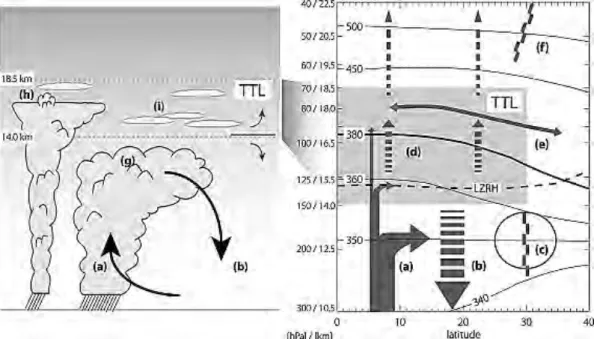
be the area where the temperature gradient changes to the point named the cold point tropopause (CPT). The tropopause can be considered as a level (as defined by the World Meteorological Organization (WMO)) or as a layer (Gettelman and Fothers, 2002; Mehta et al., 2008; Birner and Charlesworth, 2017). In this thesis, we consider the tropical tropopause as an intermediate layer around the tropical CPT, between 14 and 18.5 km above sea level (150 and 70 hPa, respectively) Fueglistaler et al. (2009a) named the TTL as tropical tropopause layer. Figure 1.1 from Fueglistaler et al. (2009a) illustrates the tropospheric cloud processes and zonal mean circulation in the tropics during deep convective activity.
The main atmospheric component transported by air masses during deep con-vective activity is water (through the vapour, liquid and solid phases as a function
of the pressure and temperature reached). Water vapour (WV) is one of the
main greenhouse gases and has an important impact on the radiative balance of the troposphere, the stratospheric ozone, and thus on the climate, particularly in the tropics. The WV distribution in the tropical upper troposphere (UT) (Soden et al., 2008) and stratosphere (Solomon et al., 2010) is strongly coupled to the distribution of thin cirrus clouds composed of ice crystals, known as having a significant effect on the overall thermal balance of the troposphere (Zhou et al., 2014). However, the way in which WV and ice travel from the troposphere to the lower stratosphere in the tropics is still poorly understood.
At the surface, evaporation and evapotranspiration release water vapour in the atmosphere. Warm air masses become lighter than the environment and start to rise up in the troposphere. With the ascent and the decrease of pressure and tem-perature, the water vapour contained in the air masses can start to condensate. Water particles continue to rise up as long as the particles are light enough. Oth-erwise, condensed water particles fall down to the surface. Near the TTL, WV and ice concentrations are controlled by temperature which regulate the
satura-1.1. INTRODUCTION (ENGLISH)
Figure 1.1 – Schematic (left) of cloud processes and transport and (right) of zonal mean circulation. Arrows indicate circulation, black dashed line is clear-sky level of zero net radiative heating (LZRH), and black solid lines show isentropes (in K, based on European Centre for Medium Range Weather Forecasts 40-year re-analysis (ERA-40)). The letter a indicates deep convection: main outflow around 200 hPa, rapid decay of outflow with height in tropical tropopause layer (TTL), and rare penetrations of tropopause. Fast vertical transport of tracers from bound-ary layer into the TTL. The letter b indicates radiative cooling (subsidence). The letter c indicates subtropical jets, which limit quasi-isentropic exchange between troposphere and stratosphere (transport barrier). The letter d indicates radiative heating, which balances forced diabatic ascent. The letter e indicates rapid merid-ional transport of tracers and mixing. The letter f indicates the edge of the “trop-ical pipe,” relative isolation of tropics, and stirring over extratropics (“the surf zone”). The letter g indicates deep convective cloud. The letter h indicates the convective core overshooting its level of neutral buoyancy. The letter i indicates ubiquitous optically (and geometrically) thin, horizontally extensive cirrus clouds, often formed in situ. Note that the height-pressure-potential temperature relations shown are based on tropical annual mean temperature fields, with height values rounded to the nearest 0.5 km. Figure 1 from Fueglistaler et al. (2009a)
tion mixing ratio in air masses (Hartmann et al., 2001; Fueglistaler et al., 2009a; Khaykin et al., 2013), decreasing the WV concentration and increasing ice parti-cles. Thus, the ratio between WV and ice crystals in convective clouds strongly
varies with altitude. However, the vertical distribution of WV over ice ratio is still not well understood, particularly in the upper troposphere and close to the TTL where i) the cold point effect plays on the water budget phase changes with micro-physics processes and ii) the troposphere to stratosphere air masses ex-changes impact the water budget in the TTL (Gettelman and Fothers, 2002; Corti et al., 2006; Dauhut, 2016).
Two major processes have been identified to control the humidification of TTL. Firstly, a slow and large-scale process, controlled by the radiative heating of the air masses, allowing to gain buoyancy and cross the cold point by about 300 m per month (Corti et al., 2006). This transport contributes to the circulation of Brewer-Dobson (Corti et al., 2006). Secondly, a rapid (1 day) and small scale process of the deep convection, named overshoots, is defined by the direct transport of air masses from the top of the deep convective cloud to the lower stratosphere (Adler and Mack, 1986; Danielsen, 1982; Dessler, 2002; Fueglistaler et al., 2009a). Overshoot can have a significant impact on the composition of the stratosphere. However, it has been shown that only a small part (∼ 18%) of water mass flux from cloud overshoot are irreversibly transported in the stratosphere (Dauhut et al., 2015), the remaining falls back into the troposphere because of the stratification.
The goal of this thesis is to improve our knowledge on thewater budget in the
TTL. Ice and water vapour in the upper troposphere and near the CPT are studied separately in relation with the deep convective activity in the tropics to provide information on the impact of the deep convection on the vertical and horizontal distribution of the water budget in the TTL. This thesis focuses more particularly
1.1. INTRODUCTION (ENGLISH)
to estimate the amount of ice injected by deep convection up to the TTL over
tropical convective areas and during convective seasons. To achieve this objective, the thesis uses firstly observational datasets from satellites, and then complete the study with meteorological reanalysis and meso-scale model datasets.
Ice water content (IWC), WV, temperature and relative humidity with
re-spect to ice, are provided from theMicrowave Limb Sounder (MLS) instrument
on board the Aura satellite in the upper tropopshere and near the CPT (146 hPa, 100 hPa) during 2004-2017. One of the main drawbacks of the MLS observa-tions where studying the diurnal cycle is its low temporal resolution. Crossing the tropics at two fixed times, MLS provides IWC and WV at 01:30 local time (LT) and 13:30 LT. IWC from MLS will also be compared to IWC measured at high (1-hour) temporal resolution from the Superconducting Submillimeter-Wave Limb-Emission Sounder (SMILES) during the short period provided by the in-strument (April 2009 to October 2010). In order to study the impact of deep
con-vection on ice and WV up to TTL, firstly precipitation from theTropical Rainfall
Measuring Mission (TRMM) 3B42 algorithm (TRMM-3B42), averaged at high (1-hour) temporal resolution during the same study period as MLS and over the
all tropical band (30◦S, 30◦N), is used and combined with the MLS datasets.
Sec-ondly, the deep convective activity is also studied by considering the number of flashes from lightnings provided from the Lightning Imaging Sensor (LIS) instru-ment on TRMM, from 2004 to 2015 at 1-hour resolution. Finally, IWC from the ERA5 meteorological reanalysis and the non-precipitating ice (MRI) from Meso-NH mesoscale model are compared to observation datasets to evaluate the capac-ity of the model of the meteorological analysis to reproduce the measured amount of ice injected up to the TTL from deep convection.
This study takes place within the TEASAO (Turbulence Effects on Active Species in Atmosphere, http://www.legos.obs-mip.fr/projets/
axes-transverses-processus/teasao, last access: June 2019) project lead by Dr Yves Morel and Professor Peter Haynes. The goal of the project is the preparation of the next generation of prediction and climate systems for both the atmosphere and the ocean. The challenge of this project is to answer societal problems of water resources, air and water pollution by improving models and knowledges regarding small-scale turbulences and vertical mixing of chemical and biological species in atmosphere and ocean. Theoretical and applied studies compose the project. The project is based on four teams from the LEGOS (Laboratoire d’Etudes en Géophysique et Océanographie Spatiales), the LA (Laboratoire d’Aerologie) and the CNRM (Centre National de Recherches Météorologiques) and welcomes for four years Professor Peter Haynes (from University of Cambridge (UK)) who is an international expert on atmospheric and oceanic dynamics and on transport and mixing of trace species.
The manuscript is separated in several chapters.
•Chapter 2 provides an overview on the tropospheric and stratospheric
struc-ture and composition. Tropical atmospheric dynamical processes are detailed
and deep convective activity processes are presented. A focus on the water budget in the tropical troposphere and tropopause layer is drawn.
• Chapter 3 introduces some backgrounds on remote sensing observations
and presents the instruments and the reanalysis and meso-scale model used in this thesis to estimate the amount of ice injected in the TTL during the austral convec-tive season of December, January and February (DJF) over the tropics (chapter 4) and over the named Maritime Continent region (chapter 5) and considering the Madden-Julian Oscillations (MJO) and the El Nino Southern Oscillation (ENSO) periods (chapter 6).
1.1. INTRODUCTION (ENGLISH) Physics (ACP) (Dion et al., 2019). It evaluates the mechanisms affecting the
di-urnal cycle of water budget in the TTL over the tropics. Amethod is developed
combining MLS and TRMM observations to estimate theamount of ice injected
(∆IWC) by deep convection up to the TTL. Precipitation is shown to be a good proxy of deep convection over convective regions and during the convective pe-riod. The model is validated using IWC from the SMILES instrument providing the diurnal cycle of IWC in the troposphere and tropopause layer during less than one year (October 2009 to April 2010). Finally, ∆IW C is estimated over several convective tropical oceanic and continental regions at 146 hPa in the UT and at 100 hPa in the tropopause layer (renamed TL).
• Chapter 5 is based on the article submitted and revised in ACPD (Dion et
al, 2020), focusses on the tropical region where ∆IWC is the highest namely
the Maritime Continent [15◦S – 10◦N; 90◦W – 150◦W] that includes
Indone-sia. ∆IWC is studied at high horizontal resolution (2◦ × 2◦ which represent ∼
200 × 200 km) separating ∆IWC over islands and seas of the Maritime Conti-nent. Combined with precipitation from TRMM, we also use another proxy of deep convection, the number of flashes from TRMM-LIS. The observed ∆IWC over island and seas of the Maritime Continent. Finally, the observational range of ∆IWC is finally compared to ∆IWC estimated from ice provided by ERA5 meteorological reanalyses.
•Chapter 6 shows ∆IWC estimated over the Maritime Continent during
con-vective periods governed by the Madden Julian Oscillation (MJO) and the
South-ern El Nino Oscillations (ENSO) in order to identify processes related to
intra-seasonal oscillations on the amount of ice injected from deep convection in the TTL. Observed ∆IWC during MJO is compared to ∆IWC estimated from the Meso-NH MRI datasets simulated for an MJO episodes of November 2011.
con-vection over an extra-tropical region known to be efficient for injecting air masses
in the UTLS, namely Asia, during theAsian Monsoon from June to August (JJA).
The study is based on the model developed in the thesis with precipitation and the number of flashes from TRMM as proxies of deep convection and IWC from MLS. This work has been done in parallel to the present thesis within the frame-work of the Cyrille Dallet’s Master 2 internship, supervised by Philippe Ricaud and myself.
• Conclusions are finally drawn and present some perspectives based on the
Introduction (Français)
1.2 Introduction (Français)
La convection profonde tropicale est le principal processus de transport des
masses d’air de la surface vers la haute troposphère et même jusqu’à la basse stratosphère dans les tropiques (Folkins et al., 2006; Fueglistaler et al., 2009a). Ce transport vertical joue un rôle sur la composition et la dynamique de l’atmosphère globale. On sait que ce transport est influencé par les propriétés de surface et que le cycle diurne de la convection profonde diffère sur les terres de sur les océans tropicaux (Liu and Zipser, 2005). L’altitude atteinte par le nuage tropical de con-vection profonde est crucial pour la compréhension de la distribution des masses d’air atmosphériques. Lorsque la convection n’atteint pas la stratosphère, les masses d’air sont affectées par le refroidissement radiatif et s’abaissent. Cepen-dant, lorsque la convection profonde tropicale atteint la stratosphère, les masses d’air peuvent être réparties vers les hautes latitudes suivant la circulation de Brewer-Dobson (Brewer, 1949; Holton et al., 1995; Butchart, 2014). La transition entre la troposphère et la stratosphère, appelée tropopause, est une zone atmo-sphérique clé qui contrôle la distribution verticale de la température des masses d’air, des nuages, de la vapeur d’eau et de la glace. La tropopause fait l’objet de nombreuses études en raison de sa particularité d’être la zone où le gradi-ent de température change au point appelé le point froid de la tropopause (CPT
pour "cold point tropopause"). La tropopause peut être considérée comme un niveau (tel que défini par l’Organisation météorologique mondiale (WMO)) ou comme une couche atmospherique (Gettelman and Fothers, 2002; Mehta et al., 2008; Birner and Charlesworth, 2017). Dans cette thèse, nous considérons la tropopause tropicale comme une couche intermédiaire autour du CPT tropical, entre 14 et 18,5 km au-dessus du niveau de la mer (respectivement entre 150 et 70 hPa), (Fueglistaler et al., 2009a), désignée par le terme générique TTL pour "Tropical Tropopause Layer". La Figure 1.2 de Fueglistaler et al. (2009a) illustre les processus des nuages troposphériques et la circulation moyenne zonale dans les tropiques au cours des périodes suivant une activité convective profonde.
Le principal composant atmosphérique transporté par les masses d’air pen-dant l’activité convective profonde est l’eau à travers les phases vapeur, liquide et
solide en fonction de la pression et de la température atteinte. Lavapeur d’eau
(WV pour "water vapour") est l’un des principaux gaz à effet de serre et a un impact important sur l’équilibre radiatif de la troposphère, mais aussi sur l’ozone stratosphérique et donc sur le climat, en particulier sous les tropiques. La distribu-tion de la WV dans la haute troposphère tropicale (UT pour "upper troposphere") (Soden et al., 2008) et dans la stratosphère (Solomon et al., 2010) est fortement liée à la distribution spatiale des fins nuages composés de cristaux de glace (les cirrus), connus pour avoir un effet significatif sur le bilan radiatif global de la tro-posphère (Zhou et al., 2014). Cependant, la façon dont la WV et la glace sont transportées de l’UT dans la basse stratosphère (LS pour "lower stratosphere") sous les tropiques est toujours mal comprise.
En surface, l’évaporation et l’évapotranspiration libèrent de la vapeur d’eau dans l’atmosphère. Les masses d’air chaudes deviennent plus légères que l’environnement et commencent à s’élever dans la troposphère. Avec la montée en altitude et la baisse de la pression et de la température, la vapeur d’eau contenue
1.2. INTRODUCTION (FRANÇAIS)
Figure 1.2 – Schéma (à gauche) des processus et du transport des nuages et (à droite) de la circulation moyenne zonale. Les flèches indiquent la circulation, la ligne pointillée noire correspond au niveau de chauffage radiatif nul en ciel clair (LZRH) et les lignes pleines noires indiquent les isentropes (en K, basée sur la réanalyse sur 40 ans du Centre européen pour les prévisions météorologiques à moyenne portée (ERA-40)). La lettre a indique le processus de convection profonde : son écoulement principal est autour de 200 hPa, une décroissance rapide de l’écoulement se produit avec la hauteur dans la couche tropicale de la tropopause (TTL), laissant apparaitre de rares pénétrations de la tropopause. Dans la tropopause, on retrouve de rapide transports verticaux des masses d’air depuis la couche limite jusqu’à la TTL. La lettre b indique le refroidissement radiatif (affaissement). La lettre c indique les jets subtropicaux, qui limitent les échanges quasi-ontropiques entre la troposphère et la stratosphère (barrière de transport). La lettre (d) indique l’ascension diabatique forcée, équilibrée par le chauffage radiatif. La lettre (e) indique un transport méridien rapide des traceurs et du mélange. La lettre f indique "la zone de surf", la zone où se produit l’isolement relatif des tropiques face à l’agitation des extratropics. La lettre (g) indique un nuage convectif profond. La lettre (h) indique que le noyau convectif a dépassé son niveau de flottabilité neutre. La lettre (i) indique des cirrus omniprésents, op-tiquement et géométriquement fins, étendus horizontalement, souvent formés in situ. Notez que les relations hauteur-pression-température potentielle sont basées sur les moyenne annuelle tropicale de température, les altitudes étant arrondies au 0,5 km le plus proche. Figure 1 d’après Fueglistaler et al. (2009a)
dans les masses d’air ascendantes peut commencer à condenser. Les particules d’eau continuent de monter tant qu’elles sont suffisamment légères. Sinon, des particules d’eau condensées tombent à la surface par gravité. Près de la TTL, les concentrations de WV et de glace sont contrôlées par les très faibles température qui régulent le rapport de mélange de saturation dans les masses d’air (Hartmann et al. 2001 ; Fueglistaler et al., 2009 ; Khaykin et al., 2013), réduisant la concen-tration de WV et augmentant les particules de glace. Ainsi, le rapport entre la WV et les cristaux de glace dans les nuages convectifs varie fortement avec l’altitude. Cependant, la distribution verticale du rapport WV sur glace n’est pas encore bien comprise, en particulier dans la haute troposphère et à proximité du TTL où i) l’effet du point froid joue sur les changements de phase du bilan hydrique avec la microphysique et ii) les échanges entre la troposphère et les masses d’air de la stratosphère ont un impact sur le bilan hydrique dans la TTL (Gettelman et Fothers, 2002 ; Corti et al., 2006 ; Dauhut, 2016).
Deux processus majeurs ont été identifiés pour contrôler l’humidification de la TTL. Tout d’abord, un processus lent et à grande échelle, contrôlé par le réchauf-fement radiatif des masses d’air, et permettant aux masses d’air de franchir le point froid à une vitesse d’environ 300 m par mois (Corti et al., 2006). Ce trans-port contribue à la circulation de Brewer-Dobson (Corti et al., 2006). Deuxième-ment, un processus rapide (∼ 1 jour) et à petite échelle de la convection pro-fonde, appelé percées nuageuses (overshoots en anglais), est défini par le trans-port direct des masses d’air du sommet du nuage convectif profond vers la basse stratosphère (Adler and Mack, 1986; Danielsen, 1982; Dessler, 2002; Fueglistaler et al., 2009a). Le dépassement peut avoir un impact significatif sur la composition de la stratosphère. Cependant, il a été démontré que seule une petite partie (∼ 18%) du flux massique d’eau provenant de la surabondance des nuages est trans-portée de façon irréversible dans la stratosphère (Dauhut et al., 2015), le reste
1.2. INTRODUCTION (FRANÇAIS) retombe dans la troposphère en raison de la stratification.
Le but de cette thèse est d’améliorer nos connaissances sur lebilan hydrique
dans la TTL. La glace et la vapeur d’eau dans la haute troposphère et à proximité du CPT sont étudiées séparément en relation avec l’activité convective profonde dans les tropiques pour fournir des informations sur l’impact de la convection pro-fonde sur la distribution verticale et horizontale du bilan en eau dans le TTL. Cette
thèse porte plus particulièrement sur la phase solide de l’eau et sur les processusà
l’échelle diurne afin d’estimer la quantité de glace injectée par convection pro-fonde jusqu’à la TTL sur les zones tropicales convectives et pendant les saisons convectives. Pour atteindre cet objectif, la thèse utilise d’abord des jeux de don-nées d’observation provenant de satellites, et complète l’étude par des dondon-nées
deréanalyse météorologique et des données de modèle de méso-échelle.
Lateneur en eau glacée (IWC pour "ice water content" en anglais), la WV,
la température et l’humidité relative par rapport à la glace sont fournies par
l’instrument MLS (Microwave Limb Sonder) à bord du satellite Aura dans la
haute troposphère (146 hPa) et près du CPT (100 hPa) durant la période d’étude de 2004 à 2017. L’un des principaux inconvénients des observations MLS lorsque l’on étudie le cycle diurne d’un élément est sa faible résolution temporelle. Sur-volant les tropiques à deux heures locales fixes, MLS fournit IWC et WV à 01:30 heure locale (LT pour local time en anglais) et 13:30 LT. IWC fournie par MLS sera également comparée à IWC mesurée à une résolution temporelle élevée (1 heure) par l’instrument SMILES (Superconducting Submillimeter-Wave Limb-Emission Sounder) à bord de la station spatiale internationale pendant la courte période de mesure fournie par l’instrument (d’avril 2009 à octobre 2010). Afin d’étudier l’impact de la convection profonde sur la glace et la WV jusqu’à la TTL, on utilise d’abord les précipitations fournies à partir des mesures du
(TRMM-3B42), dont la résolution temporelle moyenne est élevée (1 heure). TRMM-3B42 est utilisé pendant la même période d’étude que MLS et sur toute
la bande tropicale (30◦S – 30◦N). Les données sont ensuite combinées aux jeux
de données MLS. Deuxièmement, l’activité convective profonde est également étudiée en considérant le nombre d’éclairs durant les événements orgareux four-nis par l’instrument LIS (Lightning Imaging Sensor) à bord de la plateforme TRMM, de 2004 à 2015 avec une résolution d’une heure. Enfin, IWC fournie par les réanalyses météorologiques de ERA5 et la glace non précipitante (MRI pour "mixing ratio ice") fournie par le modèle de méso-échelle, Méso-NH, sont comparées aux jeux de données d’observation afin d’évaluer la capacité du modèle et des analyses météorologiques à reproduire la quantité mesurée de glace injectée jusqu’à la TTL par convection profonde.
Cette étude a lieu dans le cadre du projet TEASAO (Turbulence Ef-fects on Active Species in Atmosphere, http://www.legos.obs-mip.fr/projets/axes-transverses-processus/teasao, dernier accès : juin 2019) dirigé par le Dr Yves Morel (LEGOS, France) et le Professeur Peter Haynes (DAMTP, Cambridge, G-B). Le but du projet est de préparer la prochaine génération de systèmes de prévi-sion et de systèmes climatiques pour l’atmosphère et l’océan. Le défi de ce projet est de répondre aux problèmes sociétaux de ressources en eau, de pollution de l’air et de l’eau en améliorant les modèles et les connaissances concernant les turbu-lences à petite échelle et le mélange vertical des espèces chimiques et biologiques dans l’atmosphère et l’océan. Quatre projets basés sur des études théoriques et ap-pliquées composent le projet et s’appuient sur quatre équipes du LEGOS (Labora-toire d’Etudes en Géophysique et Océanographie Spatiales), du LA (Labora(Labora-toire d’Aerologie) et du CNRM (Centre National de Recherches Meteorologiques). Il vise aussi à s’appuyer sur l’expertise internationale du Professeur Peter Haynes (Université de Cambridge) dans les domaines de la dynamique atmosphérique et
1.2. INTRODUCTION (FRANÇAIS) océanique et du transport et mélange des éléments traces en l’accueillant pendant quatre ans à l’OMP à Toulouse.
Le manuscrit est séparé en plusieurs chapitres.
• Le chapitre 2 donne un aperçu de la structure et de la composition
tro-posphériques et stratosphériques. Les processus dynamiques atmosphériques
tropicaux sont détaillés et les processus d’activité convective profonde sont présentés. L’accent est mis sur le bilan hydrique dans la troposphère et la tropopause tropicale.
•Le chapitre 3 présente les observations de télédétection ainsi que les
instru-ments et les réanalyses meteorologiques et le modèle de méso-échelle utilisés dans cette thèse afin d’estimer la quantité de glace injectée dans le TTL pendant la saison convective australe de décembre, janvier et février (DJF) sur les tropiques (chapitre 4) et sur la région dénommée Continent Maritime (chapitre 5) en con-sidérant aussi les oscillations à large échelle: Oscillations Madden-Julian (MJO) et El Niño Southern Oscillation (ENSO) (chapitre 6).
•Le chapitre 4 est basé sur l’article publié dans Atmospheric Chemistry and
Physics (ACP) (Dion et al., 2019). Il évalue les mécanismes affectant le cycle
diurne du bilan hydrique dans le TTL sous les tropiques. Uneméthode est mise
au point combinant les observations MLS et TRMM pour estimer la quantité de glace injectée (∆IW C) par convection profonde jusqu’à la TTL. Les précipita-tions se révèlent être un bon indicateur de la convection profonde dans les régions convectives et pendant la période convective. Le modèle est validé à l’aide de IWC mesurée par l’instrument SMILES qui fournit le cycle diurne de IWC dans la tro-posphère et la tropopause avec un pas de temps de 1 heure d’octobre 2009 à avril 2010. Enfin, ∆IW C est estimée sur plusieurs régions convectives océaniques et continentales dans les tropiques dans l’UT à 146 hPa et dans la tropopause (nommé TL) à 100 hPa.
• Le chapitre 5 est basé sur l’article soumis et révisé à ACPD (Dion et al., 2020), se concentre sur la région tropicale où on a montré que ∆IW C était la
plus élevée, à savoir leContinent Maritime [15◦S – 10◦N ; 90◦W – 150◦W] qui
inclut l’Indonésie. ∆IW C est étudiée à haute résolution horizontale (2◦ × 2◦
ce qui représente ∼ 200 × 200 km) en distinguant les îles et mers du Continent Maritime. En complément des précipitations fournies par TRMM, nous utilisons également une autre approximation de la convection profonde, le nombre d’éclairs durant les évènements orageux fourni par l’instrument LIS du satellite TRMM pour caractériser ∆IWC au-dessus des îles et mers du Continent Maritime. Enfin,
∆IW C estimée à partir des données d’observations satellitaires est comparée à
∆IW C estimée à partir des données de teneur en eau glacée fournies par les
réanalyses météorologiques ERA5.
• Le chapitre 6 est composé de l’étude de ∆IW C estimée sur le Continent
Maritime pendant les périodes convectives régies par l’oscillation Madden-Julian (MJO) et les oscillations La Nina afin d’identifier l’impact des processus liés aux oscillations intra-saisonnières et inter-annuelles sur la quantité de glace injec-tée dans la TTL. ∆IW C estimée à partir des observations pendant la MJO est comparée à ∆IW C estimée à partir des jeux de données de glace fournis par le modèle de meso-échelle Meso-NH, simulée pour un épisode de MJO de novembre 2011.
•Le chapitre 7 présente l’étude de la quantité de glace injectée jusqu’à la TTL
par convection profonde sur une région extra-tropicale connue pour son efficacité
à injecter des masses d’air dans l’UTLS, notamment en Asie, pendant lamousson
asiatique de juin à août (JJA). L’étude est basée sur le modèle développé dans la thèse utilisant les précipitations et le nombre d’éclairs fournis par TRMM comme approximations de la convection profonde et IWC fournie par MLS. Ce travail a été réalisé en parallèle à la présente thèse dans le cadre du stage de Master 2 de
1.2. INTRODUCTION (FRANÇAIS) Cyrille Dallet, encadré par Philippe Ricaud et moi-même.
• Des conclusions sont enfin tirées et quelques perspectives basées sur les
Chapter 2
Fundamentals in atmospheric
physics and chemistry
This chapter provides an overview on the tropospheric and stratospheric structure and composition. Transport and processes controlling tropical deep convection and its internal structure, mechanism and impacts are detailed. A focus on the definition of tropopause and on the tropical troposphere to stratosphere exchanges as well as on the water budget in these atmospheric layers is overviewed. Some basic meteorological concepts and terminology specific to the study of tropical deep convection are recalled.
2.1 Structure of the atmosphere and tropopause
definitions
2.1.1 Global atmospheric structure
The atmosphere is an envelope of gas surrounding the Earth. Because of gravity, the density of the atmosphere is higher at the surface than in altitude, meaning
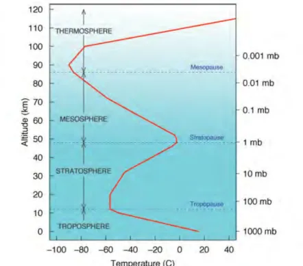
that pressure decreasing with altitude. Figure 2.1 presents the atmospheric struc-ture and temperastruc-ture profile: each altitude of temperastruc-ture inversion defines the separation between two layers. Because of the chemical composition of the atmo-sphere, the temperature profile changes with altitude. The layer extending from the surface to 7-15 km is called the Troposphere. This layer is the thinnest layer but contains about 80 % of atmosphere’s total mass and about 99% of the
atmo-sphere’s total water vapour. Temperature decreases by about -3 to -10 K km-1
with altitude according do the Ideal Gas Law because pressure decrease with al-titude. Vertical turbulent mixing is relatively frequent in this layer. The top of the troposphere is called the tropopause where temperature reaches a minimum, called the cold point tropopause (CPT). Then, temperature increases with altitude in the layer above the tropopause, called the Stratosphere. Thus, the tropopause is the level of transition between the two layers and will be defined precisely in sections 2.1.2 and 2.1.3. In the stratosphere, the temperature increases from 1 to
3 K km-1, and the layer can be defined between 10 and 50 km of altitude. This
layer has got the particularity of containing the greatest part of the ozone (O3), in
a intra-layer (called the ozonophere, with a maximum around 25 km of altitude).
The amount of O3 in the stratosphere is an important for the protection of living
organisms, by absorbing most of the sun’s ultraviolet radiation. Higher than the stratosphere, the mesosphere is found between 50 and 80 km, with temperature decreasing with height up to the mesopause where temperature is the lowest in at-mosphere. Above, the thermosphere reaches an altitude up to 620 km. This layer accommodates boreal aurora and the International Space Station.
2.1.2 Tropopause, a level: thermal and dynamical definitions
The tropopause can be considered as a level or a layer. This section present the definition of the tropopause level. The level of the tropopause is defined by a
2.1. STRUCTURE OF THE ATMOSPHERE AND TROPOPAUSE DEFINITIONS
Figure 2.1 – Schematic representation of the atmospheric structure and
tempera-ture (◦C) profil (red) as a function of altitude (km) and pressure (mb).
Source: c 2006. Steven C. Wofsy, Abbott Lawrence Rotch Professor of
Atmo-spheric and Environmental Science, lecture notes.
minimum of temperature (Figure 2.1). In the troposphere, an air parcel rises adi-abatically, cools down and expands with altitude up to high altitudes with cold temperatures such as in the troposphere top. In the stratosphere, because of the
large O3content, which absorbs the solar ultra violet (UV) radiation and converts
it to heat, temperature is back to increase with altitude. However, the level of the tropopause is used to be defined, in the extratropics, by the concept of dy-namical tropopause through potential vorticity surfaces. More precisely, as the tropopause can be considered as a boundary, separating troposphere and strato-sphere dynamical processes, numerical models have defined the tropopause as the break of the variability of the potential vorticity (PV). The PV describes the value of an air masses vorticity between two isentropic and adjacent surfaces. Thus, the
tropopause is defined as the altitude where the PV is about 2.10-6K m2kg-1.s-1(or
2.0 PV Unit (PVU)). In the tropics, the PV cannot be measured because of the PV surface goes to zero near the equator (Hoinka, 1998). Thus, within the tropics, the thermal definition is the only applicable criterion. Hoinka (1998) used both def-inition of the tropopause (thermal and PV defdef-initions) to get a global tropopause profile, as shown in Figure 2.2. Figure 2.2 illustrates the annual mean merid-ional profile of the zonally-averaged tropopauses (1979-93; 1200UTC): thermal tropopause (THE); dynamical tropopause with PV = 1.6 (PV1), PV = 2.5 (PV2), and PV = 3.5 (PV3) PVU, from Hoinka (1998).
Figure 2.2 – Annual mean meridional profile of the zonally-averaged tropopauses (1979-93; 1200UTC): thermal tropopause (THE); dynamical tropopause with 1.6 (PV1), 2.5 (PV2), and 3.5 (PV3) PVU. (Hoinka, 1998)
Following the World Meteorological Organization (WMO), the tropopause level is also defined as the lowest level at which the lapse rate decreases to 2
K km-1 or less, that is, the average lapse rate between this specific level and all
higher levels within 2 km does not exceed 2 K km-1.
2.1. STRUCTURE OF THE ATMOSPHERE AND TROPOPAUSE DEFINITIONS
Tropical Extra-tropical
Temperature Colder (-80°C) Warmer (-60°C)
Latitudinal
extension Between the two subtropical jet streams Between subtropical and polar jet streams
Height 18 km (80-100 hPa) 12 km (200-300 hPa)
Annual cycle
altitude Low amplitude of the annual cycle (lower in summer and higher in
winter from 0° to 10° N, and the opposite signal from 0° to 10°S)
Higher in summer and lower in winter
Radiation Radiative convective balance Baroclinic wave dynamics
Vertical transport Upward circulation Downward circulation
Table 2.1 – Characteristics of tropical and extratropical tropopauses streams. The change in horizontal temperature in a frontal zone creates a pres-sure variation at a given altitude. This tropospheric prespres-sure variation helps the increase of winds with altitude up to the tropopause level. The jets tends to be where the tropopause is more vertical than horizontal (see in Figure 2.3). In the stratosphere, however, the variation is opposite and the wind decreases. Thus, four jet streams characterizing the tropopause have been identified: the Arctic, the polar, the subtropical, and the equatorial jet streams (see in Figure 2.3).
Fur-thermore, if above the tropopause, the temperature gradient reaches -3◦C km-1,
then it is possible to define a second tropopause (as illustrated in Fig. 2.3). Thus, the troposphere can be separated to the stratosphere by multiples tropopauses as defined using the lapse rate definition (Randel et al., 2007). This phenomenon is observed is all season, all longitudes and mainly in the mid-latitude (Wang and Polvani, 2011).
Table 2.1 synthesizes specific differences between the tropical and the extrat-ropical tropopauses. As shown in Table 2.1, the altitude and the temperature of
the tropopause change as a function of the latitude and longitude (Randel et al., 2006b; Fueglistaler et al., 2009a; Suneeth et al., 2017), but it can be averaged
around 4-6 km (≈ 300 hPa) and -65◦C in polar regions, 8-12 km (≈ 200 hPa) and
near -55◦C in both hemispheres and around 15-18 km (≈ 100 hPa) and -85◦C in
the tropics (Rieckh et al., 2014; Graversen et al., 2014)). The latitudinal variation of the tropopause from the poles to the equator is schematically illustrated in Fig-ure 2.3 (Shapiro et al., 1987). In summer, because of the troposphere heating, the altitude of the extratropical tropopause is higher than in winter. However, while the tropopause temperature is stable, the tropopause height shows large variations with seasons, and day-to-day. Furthermore, in the tropics, the isentropic surface at 380 K is usually used as the tropopause level because this surface is located slightly above the surface representing the average level of zero radiative heating in clear sky (concept explained in detail in section 2.2.2.3).
2.1.3 Tropical Tropopause, a transition layer: the TTL
Many studies have tried to understand and define exactly what the tropopause is, and which method is the best for each region in the globe (Reed and Danielsen, 1958; Danielsen, 1959; Shapiro, 1980; Danielsen et al., 1987; Hoerling et al., 1991; Hoinka, 1998; Gettelman and Fothers, 2002; Fueglistaler et al., 2009a). Some authors define the tropopause, no longer as a level, but as a transition layer between the troposphere and the stratosphere, where an abrupt change in
tem-perature lapse rate (K km-1) usually occurs. Define the tropopause as a level has
been shown to be difficult because its thickness will vary as a function of differ-ent physical processes. For instance, Atticks and Robinson (1983) have proposed the large range of altitudes of the tropopause between 130 and 60 hPa from the study of tropical radiosonde profiles. Randel and Wu (2007) also describe the tropopause by considering that the sharp gradient in radiative cooling affecting
2.1. STRUCTURE OF THE ATMOSPHERE AND TROPOPAUSE DEFINITIONS
Figure 2.3 – Latitudinal variation of the potential vorticity discontinuity
tropopause altitude. The 40 m s-1 isotach (thin dashed line) encircles the cores
of the three jetstreams: the Artic, JA; the polar, JP; the subtropical, JS; and the
equatorial, JE. The secondary tropical tropopause shows the level of the thermal
tropopause. Fronts and the Inter-Tropical Convergence Zone (ITCZ) are marked by fine dashed lines. (Shapiro et al. (1987), Courtesy: American Meteorological Society)
the water vapour and ozone sharp gradient to the tropopause would be the main important mechanisms to sharp the tropopause.
In the tropics, because of strong convective activities (see section 2.2), the trop-ical tropopause layer presents a zone of mixing between the troposphere and the stratopshere. For that reason, and because the tropopause cannot be defined by the PV, special definitions have been given to the tropical tropopause layer (TTL). The most common definition of the TTL is from Fueglistaler et al. (2009a):
de-limited by the subtropical jets located around 30◦N and 30◦S, the layer is defined
between the surface of 150 hPa (about 350 K and 14 km) and the surface of 70 hPa (about 425 K and 18.5 km) knowing that the surface at 350 K is the level where the jets limit the horizontal transport between the tropics and the extratrop-ics (Haynes and Shuckburgh, 2000).