RESEARCH OUTPUTS / RÉSULTATS DE RECHERCHE
Author(s) - Auteur(s) :
Publication date - Date de publication :
Permanent link - Permalien :
Rights / License - Licence de droit d’auteur :
Bibliothèque Universitaire Moretus Plantin
Institutional Repository - Research Portal
Dépôt Institutionnel - Portail de la Recherche
researchportal.unamur.be
University of Namur
Symbolic dynamics in a binary asteroid system
Di ruzza, Sara; Daquin, Jerome; Pinzari, Gabriella
Published in:
Communications in Nonlinear Science and Numerical Simulation
DOI:
10.1016/j.cnsns.2020.105414
Publication date:
2020
Document Version
Peer reviewed version
Link to publication
Citation for pulished version (HARVARD):
Di ruzza, S, Daquin, J & Pinzari, G 2020, 'Symbolic dynamics in a binary asteroid system', Communications in
Nonlinear Science and Numerical Simulation, vol. 91, 105414. https://doi.org/10.1016/j.cnsns.2020.105414
General rights
Copyright and moral rights for the publications made accessible in the public portal are retained by the authors and/or other copyright owners and it is a condition of accessing publications that users recognise and abide by the legal requirements associated with these rights. • Users may download and print one copy of any publication from the public portal for the purpose of private study or research. • You may not further distribute the material or use it for any profit-making activity or commercial gain
• You may freely distribute the URL identifying the publication in the public portal ?
Take down policy
If you believe that this document breaches copyright please contact us providing details, and we will remove access to the work immediately and investigate your claim.
SARA DI RUZZA, J ´ER ˆOME DAQUIN, AND GABRIELLA PINZARI
Abstract. We highlight the existence of a topological horseshoe arising from a a–priori stable model of the binary asteroid dynamics. The inspection is numerical and uses correctly aligned windows, as described in a recent paper by A. Gierzkiewicz and P. Zgliczy´nski, combined with a recent analysis of an associated secular problem.
Contents
1. Purpose of the paper 1
2. Poincar´e mapping 7
2.1. Hyperbolic structures and heteroclinic intersections 8
3. Symbolic dynamics via covering relations 9
3.1. Covering relations and topological horseshoe 9
3.2. Existence of a topological horseshoe 12
4. Conclusions and open problems 13
Acknowledgments 14
A. The Hamiltonian 14
B. Numerical setups and results 15
B.1. Choice of the parameters 15
B.2. Flow 15
B.3. Poincar´e mapping P 16
B.4. Coordinates of the fixed–points of P 16
C. The Fast Lyapunov Indicator & dynamical timescales 17
References 19
Highlights
‚ The secular motions of binary asteroid system interacting with a planet is analysed. ‚ The perihelia of the ellipses of the asteroids afford stable unperturbed motions. ‚ A planet orbiting outside and coming close to the asteroids has a perturbing effect. ‚ The flow is reduced to a discrete map. Its phase–space is depicted.
‚ A topological horseshoe is constructed providing the existence of symbolic dynamics. Keywords: three–body problem; binary asteroid system; horseshoe and symbolic dynamics.
1. Purpose of the paper
This paper aims to highlight chaos in the secular motions of a binary asteroid system interacting with a planet whose orbit is external to the orbits of the asteroids. These chaotic motions turn to bifurcate from an a–priori stable configuration, in the sense of [1]. We shall not provide rigorous proofs, besides the heuristic arguments that we are going to present in this introduction. In fact, our study will be purely numerical. Moreover, we shall not implement any algorithm to control machine errors. We are however convinced that our computations are correct thanks to a–posteriori checks that we shall
This research is funded by the ERC project 677793 StableChaoticPlanetM.
describe in the course of the paper.
Let us describe the physical setting. Three point masses constrained on a plane undergo Newtonian attraction. Two of them (the asteroids) have comparable (in fact, equal) mass and, approximately, orbit their common barycentre. The orbit of a much more massive body (the planet) keeps external to the couple, for a sufficiently long time. We do not assume1any prescribed trajectory for any of the bodies, but just Newton law as a mutual interaction. We fix a reference frame centred with one of the asteroids and we look at the motions of the other one and the planet. As no Newtonian interaction can be regarded as dominant – as, for example, in the cases investigated in [3–7] and [8,9] – in order to simplify the analysis, we look at a certain secular system, obtained, roughly, averaging out the proper time of the reference asteroid. This means that we are assuming that the time scale of the movements of the planet is much longer. Beware that our secular problem has nothing to do with the one usually considered in the literature, where the average is performed with respect to two proper times (e.g., [10]). Let us look, for a moment, to the case where the planet is constrained on a circular trajectory. In such case, the only observables are the eccentricity and the pericentre of the instantaneous ellipse of the asteroid. Quantitatively, this system may be described by only two conjugate Hamiltonian coordinates: the angular momentum G (related to the eccentricity) and the pericentre coordinate g of the asteroidal ellipse. There is a limiting situation, which roughly corresponds to the planet being at infinite distance, where, exploiting results from [11–13], the phase portrait of the system in the plane pg, Gq reveals only librational periodic motions. Physically, such motions correspond to the perihelion direction of the asteroidal ellipse affording small oscillations about one equilibrium position, with the ellipse highly eccentric and periodically squeezing to a segment. The movements are accompanied by a change of sense of motion every half–period. The purpose of this paper is to highlight the onset of chaos in the full secular problem, when the planet is far and moves almost circularly.
The Hamiltonian governing the motions of three point masses undergoing Newtonian attraction is, as well known, H “ |y0| 2 2m0 ` |y1| 2 2µm0 ` |y2| 2 2κm0 ´ µm 2 0 |x0´ x1| ´ κm 2 0 |x0´ x2| ´ µκm 2 0 |x1´ x2| . (1.1)
Here, x0, x1, x2 and y0, y1, y2 are, respectively, positions and impulses of the three particles relatively
to a prefixed orthonormal frame pi, j, kq Ă R3; m
0, m1 “ µm0, m2 “ κm0, with yi “ mix9i, are
their respective gravitational masses; | ¨ | denotes the Euclidean distance and the gravity constant has been taken equal to one, by a proper choice of the unit system. In the sequel, in accordance to our problem, we shall take xi, yi P R2ˆ t0u » R2 and µ “ 1 ! κ, so that x0, x1 correspond to the
position coordinates of the asteroids; x2 is the planet. The Hamiltonian H is translation invariant, so
we rapidly switch to a translation–free Hamiltonian by applying the well known Jacobi reduction. We recall that this reduction consists of using, as position coordinates, the centre of mass r0of the system
(which moves linearly in time); the relative distance x of two of the three particles; the distance x1of
the third particle with respect to the centre of mass of the former two. Namely,
r0“ px0` µx1` κx2qp1 ` µ ` κq´1, x “ x1´ x0, x1 “ x2´ px0` µx1qp1 ` µq´1.
(1.2)
Note that, under the choice of the masses specified above, we are choosing the asteroidal coordinate x0 as the “starting point” of the reduction. This reverses a bit the usual practice, as x0is most often
chosen as the coordinate of the most massive body; see Figure 1. At this point, the procedure is classical: the new impulses pp0, y, y1) are uniquely defined by the constraint of symplecticity, with
p0 (“total linear momentum”) being proportional to the velocity of the barycentre. Choosing (as it
is possible to do) a reference frame centred at, and moving with, r0, so to have r0” 0 ” p0, after a
suitable rescaling, one obtains (see AppendixA) H “ 1 2m0 |y|2` σ 2m0 |y1|2´m 2 0 |x| ´ m20σ |x1` ¯βx|´ ¯ β β m20σ |x1´ βx|, (1.3)
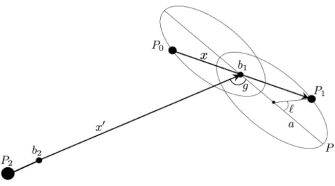
Figure 1. Schematic representation of the model we are dealing with. The model is composed by three bodies P0, P1, P2, where the first two have equal masses m0 and
the third body has the largest mass κm0, κ ą 1. The point b1 is the barycentre of
P0and P1, whilst b2is the barycentre of all the three points (close but different from
P2). with β “ κ 2 p1 ` µq µ2p1 ` µ ` κq , β “¯ κ2 p1 ` µq µp1 ` µ ` κq , σ “ κ3 p1 ` µq2 µ2p1 ` µ ` κq. (1.4)
The choice κ " µ “ 1 gives β “ ¯β " 1 and simplifies H to H “ |y| 2 2m0 ´m 2 0 |x| ` σ|y1|2 2m0 ´ m 2 0σ |x1` βx|´ m20σ |x1´ βx|. (1.5)
From now on, we regard β as mass parameter, with β „ κ and σ „ β2. By choosing a region of the phase–space where
|x1| ą |βx|, (1.6)
we ensure the denominators of the two last terms in (1.5) to be different from zero. The Hamiltonian (1.5) with x, x1, y, y1 P R2, has 4–degrees–of–freedom (DoF, from now on), but is SO(2)–invariant. We
choose a system of canonical coordinates which reduces this symmetry and hence lowers the number of DoF to 3. If k “ i ˆ j is normal to the plane of the orbits, we denote as
C “ x ˆ y ¨ k ` x1
ˆ y1¨ k
the total angular momentum, which is a constant of the motion. Then we take a 3–DoF system of coordinates, which we name pΛ, G, R, `, g, rq P R3
ˆT2ˆR, where pΛ, G, `, gq are “Delaunay coordinates for the asteroid, relatively to x1”, while pR, rq are “radial coordinates for the planet”. More precisely,
they are defined as $ ’ ’ & ’ ’ % Λ “am3 0a G “ x ˆ y ¨ k ` “ 2πSS tot g “ αx1,P , # R “ y1¨ x1 |x1| r “ |x1| (1.7)
where, considering the instantaneous ellipse generated by the first two terms in the Hamiltonian (1.5), a is the semi–major axis (see again Figure1), S and Stot are the area of the ellipse spanned from the
perihelion P and the total area and αx1,P is the angle between the direction of x1 and P relatively to
the positive direction established by x ˆ y. With these notations, ` represents the mean anomaly, G is the projection of the angular momentum of the asteroid on the direction of the unit vector k and g is the anomaly of the perihelion P with respect to the direction of x1. Using the coordinates (1.7),
condition (1.6) becomes ε ă 1 2 , ε :“ βa r (1.8)
as a body moving on an ellipse does not go further than twice the semi–axis from the focus of the ellipse. The canonical character of the coordinates (1.7) has been discussed, in a more general setting, in [11]. In terms of the coordinates (1.7), the Hamiltonian (1.5) reads
H “ ´m 5 0 2Λ2 ` σ 2m0 ´ R2`pG ´ Cq 2 r2 ¯ ´ σm 2 0 a r2` 2βarp ` β2a2%2 ´ σm 2 0 a r2´ 2βarp ` β2a2%2, (1.9)
where, for short, we have let
% “ %pΛ, G, `q “ 1 ´ e cos ξpλ, G, `q , p “ ppΛ, G, `, gq “ pcos ξ ´ eq cos g ´G
Λsin ξ sin g. Here, e “ epΛ, Gq “ c 1 ´G 2 Λ2
is the eccentricity, and ξ “ ξpΛ, G, `q denotes the eccentric anomaly, defined as the solution of Kepler’s equation
ξ ´ epΛ, Gq sin ξ “ ` .
The next step is to switch to the 2–DoF `–averaged (hereafter, secular) Hamiltonian, which we write as ¯ HpG, R, g, rq “ 1 2π ż T H d` “ ´m 5 0 2Λ2 ` σKpR, r, Gq ` σU pG, g, rq , (1.10) with KpR, r, Gq :“ R 2 2m0 `pG ´ Cq 2 2m0r2 ´2m 2 0 r U pG, g, rq :“ U`pG, g, rq ` U´pG, g, rq ` 2m20 r (1.11) where U˘pG, g, rq :“ ´m 2 0 2π ż2π 0 d` a r2˘ 2βarp ` β2a2%2. (1.12)
In (1.10) we have omitted to write Λ and C among the arguments of ¯H, as they now play the rˆole of parameters. Observe that the function U is π–periodic in g, as changing g with g ` π corresponds to swap U` and U´, as one readily sees from (1.9)–(1.12).
We do not provide rigorous bounds ensuring that the secular problem may be regarded as a good model for the full problem. Heuristically, we expect that this is true as soon as (1.8) is strengthened requiring, also,
r " β3{2a. (1.13)
Indeed, extracting r from the denominators of the two latter functions in (1.9) and expanding the resulting functions in powers of βar , one sees that the lowest order terms depending on ` have size
m20σβa r2 „ m 2 0 β3a r2 (recall that σ „ β
2). So, such terms are negligible compared to the size m20 a of the
Keplerian term, provided that (1.13) is verified. Neglecting the constant term ´m50
2Λ2 and, after a further change of time, the common factor σ in the
remaining terms, the secular Hamiltonian (1.10) reduces to ˆ
HpG, R, g, rq “ KpR, r, Gq ` UpG, g, rq . (1.14)
We now specify the range of parameters C, Λ and β and the region of the phase space for the coordinates pG, R, g, rq that we consider in this paper. In particular, we look for values of parameters and coordinates where the Hamiltonian (1.14) is weakly coupled, and describe the motions we expect to find in such region. As above, our discussion will be extremely informal.
First of all, we take Λ and C verifying
Λ ! C . (1.15)
This condition implies that also |G| ! C (as |G| ă Λ) and hence K affords the natural splitting K “ K0` K1, where K0“ R2 2m0 ` C 2 2m0r2 ´2m 2 0 r , K1“ GpG ´ 2Cq 2m0r2 . We consider a region of phase–space where r and R take values
r „ r0“ C2 2m3 0 , R „ 0 . (1.16)
These are the values where K0attains its minimum, and correspond to circular motions of the planet,
with r0being the radius of the circle. In the region of phase space defined by (1.16), the relative sizes
of K1 and U to K0 are }K1} ă c1 Λ C}K0} , } U } ă c2ε 2 }K0} , (1.17)
where ci are independent of m0, β, Λ and C. Even though (by (1.15) and (1.13)) K1and U are small
compared to K0, however, they cannot be neglected, as their sum governs the slow motions of the
coordinates G and g, which do not appear in K0. Remark that K1and U are coupled with K0, since
they depend on r. It is however reasonable to expect that, as long as the minimum of K0cages r to be
close to the value r0, the coupling is weak and the dynamics of G and g is, at a first approximation,
governed by the 1 DoF Hamiltonian
F pG, gq :“ pK1` U q|r“r0 .
(1.18)
To understand the global phase portrait of F in the plane pg, Gq, we need to recall some results from [13]. We go back to the functions U˘in (1.12), which enter in the definition of U . In [13, Section
3], it is proved that, under the assumption (1.8), the following identity holds U˘pG, g, rq “ ´m 2 0 2πr ż2π 0 p1 ´ cos ξqdξ a 1 ¯ εp1 ´ cos ξqt˘` ε2p1 ´ cos ξq2 (1.19)
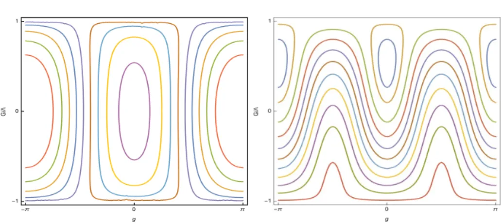
Figure 2. Left: the phase portrait of t`p¨, ¨, εq in the plane pg, G{Λq, for 0 ă ε ă 12.
Right: the phase portrait of F in the plane pg, G{Λq, with m0, C, Λ and β as in
(1.20). with ε as in (1.8) and t˘pG, g, εq :“ c 1 ´ G 2 Λ2 cos g ˘ ε G2 Λ2 .
The equality (1.19) has two main consequences. The former is that, even though the transformation (1.7) looses its meaning when G “ 0, however, U˘ keep their regularity, provided that (1.8) holds.
Indeed, the functions t˘ are regular at G “ 0 and, being bounded below by ´1 and above by 1, the denominator of the function under the integral never vanishes, under (1.8), as it is immediate to verify. Secondly, the phase portrait of the functions U`p¨, ¨, rq, U´p¨, ¨, rq coincides, a part for a
rescaling, with the one of t`p¨, ¨, εq, t´p¨, ¨, εq, respectively. In particular, U`p¨, ¨, rq and U´p¨, ¨, rq have
elliptic equilibria at pG, gq “ p0, 0q and pG, gq “ p0, πq, because this is true for t˘, as it is immediate
to check. The phase portrait of t`p¨, ¨, εq for ε ă 12 is shown in Figure2 (left); the one of t´p¨, ¨, εq is
specular, interchanging the equilibria. We now merge these informations, in order to build the phase portrait of the function F in (1.18). By the Implicit Function Theorem, one can argue that, for an open set of values of the parameters, due to the linear term in G in K1, the equilibria of U` and U´
are shifted along the G–axis, but are not destroyed. Quantifying this shift is not easy, as U has an involved dependence on t`, t´. Based on the ε–expansion of U , with
m0“ 1 , C “ 75 , Λ “
?
a “ 3 , β “ 40 (1.20)
(which comply with (1.8), (1.13), (1.15)) we obtain the phase portrait of F as in Figure2(right). We observe that, at contrast with the figure at left–hand side, where the motions are purely of elliptic kind, the phase portrait at right–hand side also includes rotational motions. The linear term of K1
is responsible of this fact, breaking the symmetry G Ñ ´G. We underline at this respect that the present framework is in a sense complementary to the one studied in [13], where the phase portrait of F has, in fact, only elliptic motions: in that case, the linear term of K1 does not exist, as C is fixed
to 0. Remark also that the vanishing of C in [13] affects condition (1.15) (which is not satisfied) and the motions generated by K0 (which are collisional, rather than circular).
The purpose of this paper is to show that, if the parameters are chosen about (1.20) and the energy is fixed to the level of a suitable initial datum pG‹, R‹, g‹, r‹q satisfying (1.16) (see AppendixB.1 for
the exact values), then, in the system (1.14) a topological horseshoe wakes up in the plane pg, G{Λq. The analysis will be purely numerical, based on techniques developed in [14], [15]. More details on the methodological strategy are given along the following sections.
2. Poincar´e mapping
From now on, we neglect to write the “hat” in (1.14). Moreover, for the purposes of the computation, we replace the function U with a finite sum
Uk “ k ÿ ν“1 qνpG, g, rq ´ βa r ¯ν (2.1)
where qνpG, g, rq are the Taylor coefficients in the expansion of U with ν “ 1, . . ., k. Using the parity
of U as a function of r, these coefficients have the form
qνpG, g, rq “ $ ’ ’ & ’ ’ % m2 0 r ν{2 ÿ p“0 ˜ qppGq cosp2p gq if ν is even 0 otherwise .
In our numerical implementation, we use the truncation in (2.1) with k “ kmax“ 10, so as to balance
accuracy and number of produced terms. We still denote as H the resulting Hamiltonian: HpG, R, g, rq “ KpG, R, rq ` UkpG, g, rq “ 1 2m0 ´ R2`pG ´ Cq 2 r2 ¯ ´2m 2 0 r ` k ÿ ν“1 qνpG, g, rq ´ βa r ¯ν . (2.2)
The study of the secular 2–DoF Hamiltonian in the continuous time t can be reduced to the study of a discrete mapping through the introduction of ad–hoc Poincar´e’s section [16]. The advantage consists in reducing further the dimensionality of the phase–space, and, in the case of n “ 2, to sharpen the visualisation of the dynamical system. In fact, for a 2–DoF system, the phase–space has dimension 4 and, due to the conservation of the energy (the Hamiltonian H itself), orbits evolve on a three– dimensional manifold M . By choosing an appropriate surface Σ transverse to the flow, one can look at the intersections of the orbits on the intersection of M X Σ, i.e., a two–dimensional surface. The surface Σ chosen is a plan passing through a given point pG‹, g‹, r‹q and normal to the associated
orbit, i.e., to the velocity vector pv‹
G, v‹g, vr‹q; it is defined by
Σ “ pG, g, rq : vG‹pG ´ G‹q ` vg‹pg ´ g‹q ` vr‹pr ´ r‹q “ 0(.
Let us now formally introduce the Poincar´e map. We start by defining two operators l and π consisting in “lifting” the initial two–dimensional seed z “ pG, gq to the four–dimensional space pG, R, g, rq and “projecting” it back to plan after the action of the flow–map Φt
H during the first return time τ . The
lift operator reconstructs the four–dimensional state vector from a seed on D ˆ T{2, where the domain D of the variable G is a compact subset of the form r´Λ, Λs. For a suitable pA, Aq Ă R2
ˆ R2, its definition reads
l : D ˆ T{2 Ą A Ñ D ˆ T{2 ˆ A z ÞÑ z “ lpzq,˜ where ˜z “ pG, g, R, rq satisfies the two following conditions:
(1) Planarity condition. The triplet pG, g, rq belongs to the plane Σ, i.e., r solves the algebraic condition v‹
GpG ´ G‹q ` vg‹pg ´ g‹q ` vr‹pr ´ r‹q “ 0.
(2) Energetic condition. The component R solves the energetic condition HpG‹, g‹, R‹, r‹q “ h‹.
The Hamiltonian is separable in R, so this condition amounts to solve a quadratic equation. If R2
ě 0, then we choose the root associated to the “positive” branch ` ?
R2. If R2
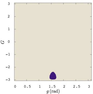
ă 0, then we are led to the notion of inadmissible seed. The set of admissible seeds, noted by A, for the chosen section Σ is portrayed in Figure3.
The projector π is the projection onto the first two components of the vector, π : D ˆ T{2 ˆ A Ñ D ˆ T{2
˜
The Poincar´e mapping is therefore defined and constructed as P : D ˆ T{2 Ñ D ˆ T{2 z ÞÑ z1“ P pzq “`π ˝ Φτ pzq H ˝ l ˘ pzq .
The mapping is nothing else than a “snapshots” of the whole flow at specific return time τ . It should be noted that the successive (first) return time is in general function of the current seed (initial condition or current state), i.e., τ “ τ p˜zq, formally defined (if it exists) as
τ pzq “ inf !
t P R`,`Gptq, gptq, rptq˘ P Σ
) , where `Gptq, gptq, rptq˘ is obtained though Φt
HpG, R, g, rq. The Poincar´e return map we described
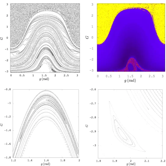
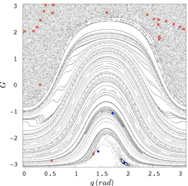
has been constructed numerically based on the numerical integration of the Hamiltonian equation of motions (the details regarding our numerical settings are presented in the AppendixB.) This mapping being now explicit, we are able to unveil the phase–space structures through successive iterations of P . Figure4presents the successive coordinates of tPnpzqu where the initial seeds z cover a discretisation of D ˆ T{2 domain (mesh) and n „ 103. The phase–space structures can be roughly categorised in three distinct zones. In the lower part, say for G ă ´2, we can distinguish one “pic” centred around g “ π{2. One elliptic zone is immersed inside this structure, surrounded by “scattered dots”, indicative of chaos. There is a large region of the phase–space foliated by circulational tori. The last upper region is a large zone where almost all regular structures have disappeared. The panel provided by Figure4 presents some magnifications of phase–space structures. The obtained phase–space structures have been confirmed using a finite time dynamical chaos indicator, the Fast Lyapunov Indicator (FLI) computed with the whole flow on an iso–energetic section (see AppendixC for more details). The FLIs computation relies on monitoring the growth over time of the tangent vector under the action of the tangent flow–map (variational dynamics). The final FLIs values are colour coded according to their values and projected onto the section to provide a stability chart. Stable orbits correspond to dark regions, orbits possessing the sensitivity to initial conditions appear in reddish/yellow color. As shown in Figure4, the FLIs confirm nicely the global structures depicted via the mapping. Moreover, numeric suggests that the lift of P on the variables pG, g, rq (i.e., the map obtained from ΦτH by
projection on pG, g, rq) is generically twist.
2.1. Hyperbolic structures and heteroclinic intersections. Equilibrium points of the mapping P (i.e., periodic orbits of the Hamiltonian system (2.2)), have been found using a Newton algorithm with initial guesses distributed on a resolved grid of initial conditions in DˆT{2 (again, see AppendixB for more details regarding the numerical setup). We found more than 20 fixed points x‹ whose coordinates have been reported in Appendix B.4. The eigensystems associated to the fixed points have been computed to determine the local stability properties. The point x‹ is hyperbolic when
one of its real eigenvalues has modulus greater than one, the other less than one (expanding and contracting directions, respectively). In the case of complex eigenvalues, the point is elliptical. The result of the analysis is displayed on Figure 5 along with the following convention: hyperbolic fixed points appear as red crosses, elliptical points are marked with blue circles. As intuitively expected, the hyperbolic points are embedded within the chaotic sea. On the contrary, the stable islands host the elliptic points. Note that even the fixed–point in the small stability island has been recovered with the Newton scheme. In the vicinity of the unstable fixed–points, the dynamics is dominated by the stable and unstable manifolds who have the eigenvectors of DP px‹q asymptotically tangents near
x‹. The local stable manifold associated to an hyperbolic point x‹,
Wloc.s px‹q “
!
x | kPnpxq ´ x‹k Ñ 0, n P N`, n Ñ 8
) ,
can be grown by computing the images of a fundamental domain I Ă Espx‹q, Espx‹q being the stable
eigenspace associated to the saddle point x‹. We considered the simplest parametrisation of I, namely
a normalised version of the eigenvector associated to the saddle point x‹. This allowed us to compute
a piece of Ws
Figure 3. The admissible points of the pg, Gq section are displayed in cream colour. They correspond to points satisfying the energetic condition H “ h‹ with R2 ě 0.
The complementary set (points leading to negative R2) appear in purple and define
the inadmissible seeds. See text for more details.
same computations are performed by reversing the time and changing Esby Eu. Finite pieces of those
manifolds are presented in Figure6for two saddle points. Following the well established conventions of the cardiovascular system (as reported in [19]), the stable manifolds are displayed with blue tones, unstable manifolds appear in red tones. As we can observe, those curves intersect transversally forming the sets of heteroclinic points, trademark of the heteroclinic tangle and chaos [20]. We now have at hands all the necessary ingredients and tools to prove the existence of symbolic dynamics using covering relationships and their images under P .
3. Symbolic dynamics via covering relations
In this section we prove the existence of symbolic dynamics for the considered model. The tools rely on ad–hoc covering relations that we present briefly following [14], in particular for the case n “ 2. 3.1. Covering relations and topological horseshoe. Let us introduce some notations. Let N be a compact set contained in R2and upN q “ spN q “ 1 being, respectively, the exit and entry dimension
(two real numbers such that their sum is equal to the dimension of the space containing N ); let cN :
R2
Ñ R2be an homeomorphism such that cNpN q “ r´1, 1s2; let Nc “ r´1, 1s2, Nc´“ t´1, 1uˆr´1, 1s,
N`
c “ r´1, 1sˆt´1, 1u; then, the two set N´“ c´1N pNc´q and N`“ c´1N pNc`q are, respectively, the exit
set and the entry set. In the case of dimension 2, they are topologically a sum of two disjoint intervals. The quadruple pN, upN q, spN q, cNq is called a h–set and N is called support of the h–set. Finally, let
SpN qlc “ p´8, ´1q ˆ R, SpN qrc “ p1, 8q ˆ R, and SpN ql “ c´1N pSpN q l
cq, SpN qr “ c´1N pSpN q r cq be,
respectively, the left and the right side of N . The general definition of covering relation can be found in [14]. Here we provide a simplified notion, suited to the case that N is two–dimensional, based on2 [15, Theorem 16].
2More precisely, Definition3.1is based on the proof of [15, Theorem 16]. Indeed, [15, Theorem 16] asserts that under
conditions (1), (3) and one of the inclusions in [15, (78) or (79)], one has Mùñ N in the sense of [f 14]. However, during the proof of [15, Theorem 16], inclusions [15, (78) or (79)] are only used to check the validity of (2).
Figure 4. Phase–space structures of the mapping P at different scales. Upper left: global phase–space; lower: microscales structures; upper right: the global phase– space analysis obtained by iterating the mapping P is confirmed by computing finite time chaos indicators based on the variational dynamics derived from the continuous model H.
Definition 3.1. Let f : R2
Ñ R2be a continuous map and N and M the supports of two h–sets. We say that M f –covers N and we denote it by M ùñ N if:f
(1) D q0P r´1, 1s such that f pcNpr´1, 1s ˆ tq0uqq Ă intpSpN qlŤ N Ť SpN qrq,
(2) f pM´qŞ N “ H,
(3) f pM qŞ N`“ H.
Conditions (2) and (3) are called, respectively, exit and entry condition.
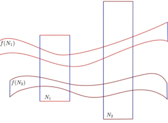
The case of self–covering is not excluded. The Figure7 shows two schematic examples of covering relation between two different sets N, M and a self–covering relation of N . The notions of covering relationships are useful in defining topological horseshoe (confer [14, 15]).
Figure 5. Phase–space of P together with its fixed–points. Hyperbolic points appear with red crosses, elliptical points appear with blue circles.
Figure 6. Finite pieces of manifolds of two hyperbolic fixed points q1, q2. Their
stable and unstable manifolds intersect transversally in (more than one) heteroclinic points. Stable manifolds are in blue while unstable manifolds are in red.
Figure 7. Examples of covering relations. On the left M
f
ùñ N . On the right, a case of self–covering N ùñ N is illustrated. In red the entry sets and their image aref represented, while in blue the exit sets and their images are represented.
Figure 8. An example of topological horseshoe where both N1, N2cover themselves
and each others. In red tones the entry sets and their images are represented, while in blue tones the exit sets and their images are represented.
Definition 3.2. Let N1 and N2 be the supports of two disjoint h–sets in R2. A continuous map
f : R2Ñ R2 is said to be a topological horseshoe for N1and N2 if
N1 f ùñ N1, N1 f ùñ N2, N2 f ùñ N1, N2 f ùñ N2.
Topological horseshoes are associated to symbolic dynamics as presented in Theorem 2 in [14] and Theorem 18 in [15], where the authors show that the existence of a horseshoe for a map f provides a semi–conjugacy between f and a shift map t0, 1uZ, meaning that for any sequence of symbols 0 and
1 there exists an orbit generated by f passing through the sets N1 and N2 in the order given by the
sequence, guaranteeing the existence of “any kind of orbit” (periodic orbits, chaotic orbits, etc.). From the Definition3.1, the covering relation N1
P
ùñ N2 is verified if the three following conditions
are satisfied:
(1) the image P pN1q of N1 lies in the strip between the top and the bottom edges of N2,
(2) the image of the left part of N´
1 lies on the left of N2,
(3) the image of the right part of N´
1 lies on the right of N2;
the conditions can be easily checked in Figure8 and, then, in Figure9.
3.2. Existence of a topological horseshoe. In this section we describe how we construct explicitly a topological horseshoe for the Poincar´e map of the Hamiltonian (1.10).
and vu, respectively, the stable and the unstable eigenvectors related to DP pqq. We construct a
parallelogram N containing q whose edges are parallel to vs and vu and thus we define N as
N “ q ` Avs` Bvu,
where A and B are suitable chosen closed real intervals. If the intervals A and B are sufficiently small, under the action of the map P , the parallelogram N will be contracted in the stable direction and expanded in the unstable direction. We denote by P pN q the image of N through the map P . In practice, we choose two hyperbolic fixed points q1 and q2 having the important property of
transversal intersection of their stable and unstable manifolds as shown in Figure 6. This property is a good indication of the existence of a topological horseshoe. Based on this couple of fixed points whose coordinates read
#
q1“ pg1, G1q “ p0.203945459, 2.06302430q,
q2“ pg2, G2q “ p0.278077917, 2.21418596q,
we define two sets N1, N2Ă R2which are supports of two h–sets as follows:
"N 1“ q1` A1vs1` B1v1u, N2“ q2` A2vs2` B2v2u, where # A1“ r´0.02, 0.08s Ă R, B1“ r´0.025, 0.01s Ă R, A2“ r´0.075, 0.025s Ă R, B2“ r´0.02, 0.01s Ă R, and vs
1, v1u, vs2, vu2 are the stable and the unstable eigenvectors related to q1, q2, respectively. Then the
following covering relations hold N1 P ùñ N1, N1 P ùñ N2, N2 P ùñ N1, N2 P ùñ N2,
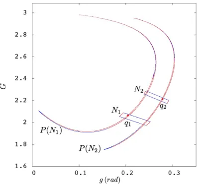
proving the existence of a topological horseshoe for P , i.e., existence of symbolic dynamics for P . The obtained horseshoe associated to q1 and q2with the aforementioned parameters is illustrated in
Figure9, providing the existence of symbolic dynamics.
4. Conclusions and open problems
This work originates from [11], where it has been pointed out that the average U` (1.12) of the
Newtonian potential with respect to one of the two mean anomalies is an integrable function which in turn may be written as a function of another function t`, whose dynamics is completely known. The
functional dependence (1.19) between these two functions, holding in the case of the planar problem, has been pointed out in [13, Section 3]. The identity (1.19) raises the very natural question whether and at which extent such relation has a consequence on the dynamics of the three–body problem. Giving an answer to such question is in fact demanding, as it requires to understand whether it is possible to find a region of phase space where the three–body Hamiltonian is well represented by its simple average (here “simple average” is used as opposite to “double average”, most often encountered in the literature, e.g., [5]) and, simultaneously, the kinetic term K in (1.11) does not interfere with U too much. In [13] it has been proved that if the total angular momentum C of the system vanishes, by symmetry reasons, and using a well–suited perturbation theory, the librational motions of t` reported in Figure2(left) have a continuation in the averaged three–body problem. In this paper we investigated the case C ‰ 0. With purely pioneering spirit, in order to simplify the analysis, we focused on the very peculiar situation where the two minor bodies have equal mass and we fixed an energy level once forever. We believe that both such choices can be removed without affecting the results too much, because, as informally discussed in the introduction, what really matters is the relative weight of K and U . Figures 2 and 4 not only show that, in our simplified model, this continuation is numerically evident, but also exhibit the onset of chaos in certain zones, clearly highlighted along
Figure 9. Horseshoe connecting the points q1 and q2 proving symbolic dynamics
for the map P . Red represents the entry sets and their images and blue the exit sets and their images.
the paper using techniques of [14]. Even though the results are encouraging, many questions are still pending (some of them have been pointed out in [13]), and we aim to face them in the future:
pQ1q If C ‰ 0, is there a choice of parameters and phase space where the phase portrait of F
includes only librational motions?
pQ2q In the case that the orbit of the planet is inner to the one of the asteroids, the phase portrait
of U` includes a saddle and a separatrix through it (see [13, Figures 1, 2 and 3]). How does
this affect the three–body problem motions?
pQ3q By [11], relation (1.19) has a generalisation to the spatial problem. What are the consequences
on the spatial three–body problem?
pQ4q Is the onset of chaos in the averaged problem present also in the full (non–secular) system?
pQ5q What can we prove analytically?
pQ6q What can we prove with computer–assisted techniques?
Acknowledgments
We are grateful to the anonymous reviewers for their stimulating remarks. We are indebted to C. Efthymiopoulos for a highlighting discussion about how to control errors (Section B.2) and to M. Guzzo for sharing his expertise on FLIs. We heartily thank U. Locatelli for an interesting talk during the meeting I-Celmech, that held in Milan, in February 2020. Figure2has been produced using the software mathematica R.
A. The Hamiltonian The impulses p0, y, y1 conjugated to r0, x, x1 in (1.2) are
p0“ y0` y1` y2 , y “ y1` µ 1 ` µy2´ µ 1 ` µp0 , y 1 “ y2´ κ 1 ` µ ` κp0 . (A.1)
If r0” 0 ” p0, the transformation of coordinates defined by (1.2) and (A.1) reduces to the injection $ ’ & ’ % x0“ ´1`µµ x ´1`µ`κκ x1 x1“ 1`µ1 x ´ 1`µ`κκ x1 x2“ 1`µ`κ1`µ x1 , $ & % y0“ ´y ´1`µ1 y1 y1“ y ´1`µµ y1 y2“ y1
and the Hamiltonian (1.1) becomes H “ 1 ` µ 2µm0 |y|2` 1 ` µ ` κ 2p1 ` µqκm0 |y1|2´µm 2 0 |x| ´ κm2 0 |x1` µ µ`1x| ´ µκm 2 0 |x1´ 1 µ`1x| . Rescaling the coordinates via
x Ñ p1 ` µqx , y Ñ µ
1 ` µy , x
1
Ñ β´1x1 , y1
Ñ µβy1,
with β as in (1.4) and multiplying the Hamiltonian H by p1 ` µq{µ, we obtain H as in (1.3). B. Numerical setups and results
B.1. Choice of the parameters. The analysis we have done is related to the choice of parameters and initial data we started with. The Hamiltonian (1.10) is composed by three parts
H “ H0` σK ` σU “: H0` P,
where the first one is the unperturbed and constant part depending on Λ, the second one represents the kinetic part and the third is the perturbing part. To ensure the non–resonant terms of P to be small with respect to H0we choose, as mentioned in the introduction,
$ ’ ’ ’ & ’ ’ ’ % m0“ 1, β “ 40, C “ 75.597 Λ “ 3.099. The initial datum is taken to be
$ ’ ’ ’ & ’ ’ ’ % G‹“ ´2.4915, R‹“ ´0.0039, g‹“ 1.4524, r‹“ 3132.069.
Note that R‹and r‹verify (1.16) but are not exactly centred at 0 and r0because the r–component of
the Hamiltonian vector–field vanishes for R “ 0, while it needs to be different from zero in order that the Poincar´e map is well defined. The values of G‹and g‹have been empirically chosen such that the
orbit from from pG‹, R‹, g‹, r‹q is approximately periodic and hence the Poincar´e map is well defined.
B.2. Flow. The Hamiltonian equations of motion have been numerically propagated using a fixed time–step RK4 method [21]. Even though the step has been kept fixed, no numerical issues have been encountered and the integration times were reasonable for the whole numeric exploration.
Under the choice of our time–step δ, the flow–map preserves the Hamiltonian itself, a conserved quantity (first integral ), with a relative error of about 10´14 for stable orbits and 10´12 for chaotic
orbits on a arc length of about τ „ 102orbital revolutions. Besides the first integral being numerically
well preserved, the quality of the integration has been assessed further using a forwards/backwards strategy. The method consists in propagating forwards in time (say on r0, τ s) the Cauchy problem
# 9
x “ vHpxq,
and then to back–propagate (from τ to 0) the new Cauchy problem
# 9
x “ vHpxq,
xpτ q “ xτ
where the initial seed xτ is obtained from the forward numerical flow–map, xτ “ Φτpx0q. Then the
relative error ∆ “ x0´ Φ´τ`Φτpx0q ˘ kx0k
is estimated. On a selection of orbits, we found ∆ to be of the order of 10´12 for regular orbits, 10´8
for chaotic orbits on timescale of about 102 orbital revolutions.
B.3. Poincar´e mapping P . The construction of the Poincar´e map P is based on the time evolution of the whole flow and a bisection procedure. Given an initial point z, to find its next state z1“ P pzq
we compute xptq “ Φt
px0q, x “ lpzq, until following conditions are met:
(1) Section condition: X “ px1ptq, x2ptq, x4ptqq P Σ up to a numerical tolerance εΣ“ 10´10. This
step relies on a bisection method halving the length of the numerical step δ until we drop under the tolerance εΣ.
(2) Orientation condition: The scalar product 9Xp0q ¨ 9Xptq is positive, meaning that the orbit is intersecting the plan Σ in the same direction as the starting point.
(3) First-return condition: for τ ă t, neither (1) and (2) are fulfilled.
B.4. Coordinates of the fixed–points of P . Below we provide the coordinates of the fixed–points of P (periodic orbits of H).
# Coordinates of the elliptic fixed points
# G g (rad)
#---2.49155 1.45245
-1.04685 1.73094 -2.91949 1.95066
# Coordinates of the hyperbolic fixed points # G g (rad) #---2.06302 0.20395 2.21419 0.27808 0.03851 0.33259 2.47589 0.34655 2.81488 0.40502 3.04924 0.43647 3.09865 0.44249 -2.84323 0.55513 2.75151 0.57177 3.05336 0.58816 3.09883 0.59055 -2.61168 1.35169 2.76024 1.61321 2.68138 2.39082 2.52039 2.51911 2.31386 2.60074 2.49651 2.61696 1.85433 2.62309 1.75010 2.62341 2.43689 2.75722 2.33537 2.90395 2.22839 3.01548
C. The Fast Lyapunov Indicator & dynamical timescales
The Fast Lyapunov Indicator (FLI) is an easily implementable tool suited to detect phase–space struc-tures and local divergence of nearby orbits. It has a long–lasting tradition with problems motivated by Celestial Mechanics [22]. The indicator can be used in the context of deterministic ODEs, map-pings, and is able to detect manifolds and global phase–space structures [23–25]. A large literature exists with the FLI tested on idealised systems (e.g., low dimensional quasi–integrable Hamiltonian system [23, 26], drift in volume–preserving mappings [27]) but also on many applied gravitational problems across a variety of scales, ranging from the near–Earth space environment [28] to exoplan-etary systems [29]. For simplicity, let us present the tool in the case of ODEs. Let us assume we are dealing with a n–dimensional autonomous ODE system. If the system is non–autonomous, we classically extend the dimension of the phase–space by 1 dimension. The FLI indicator is based on the variational dynamics in R2n,
# 9
x “ f pxq, 9
w “ Df pxq ¨ w, w P TxM , and is defined at time t as
FLIpx0, w0, tq “ sup0ďτ ďtlog kwpτ qk .
(C.1)
The FLI is able to distinguish quickly the nature of the orbit emanating from x0. Orbits containing the
germ of hyperbolicity will have their final FLI values larger than regular orbit (for the same horizon time τ ). More precisely, chaotic orbits will display a linear growth (with respect to time) of their FLIs, whilst regular orbits have their FLIs growing logarithmically. In order to reduce the parametric dependence of the FLIs upon the choice of the initial tangent vector, the FLIs are computed over an orthonormal basis of the tangent space (i.e., we compute Eq. (C.1) 4 times with a different initial w0)
and averaged [26]. As a rule of thumb, the FLI is computed over a few Lyapunov times τL, but in
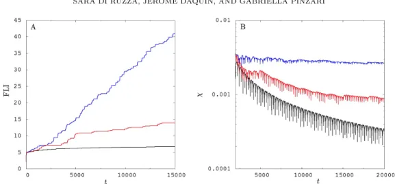
Figure 10. On the left: calibration of the finite time chaos indicators (FLI) for three distinct orbits. After a transient time of about t „ 5, 000 (i.e., „ 10 orbital revolutions) the discrimination of the nature of the orbits is sharp enough. On the right: time evolution of the maximal Lyapunov exponents χ. For chaotic orbits, they define Lyapunov timescales of about 0.76 orbital revolutions.
FLIs on discretised domains of initial conditions, the color coding of the FLIs (using a divergent color palette) reveals the global topology of the phase–space (e.g., web of resonances and preferred routes of transport, see [26]) furnishing a so–called stability map. The Lyapunov time τL is obtained as the
inverse of the maximal Lyapunov characteristic exponent (we refer to [30] for computational aspects related to characteristic exponents),
τL“ 1{χ,
where χ denotes the maximal Lyapunov characteristic exponent χpx0, w0q “ lim
tÑ`8
1
tlog kwptqk .
Stable orbits do satisfy χ Ñ 0 and hence τL tends to be large. On the contrary, chaotic orbits are
characterised by χ Ñ r P R‹
` and therefore τL converges to a finite value. The panel shown in
Figure10presents the calibration procedure based on three orbits. The stable orbit displayed in black (logarithmic growth of the FLI) admits for initial condition pG, gq “ p´2, πq. The two others orbits are chaotic but one (red) is less hyperbolic than the other (blue). The respective initial conditions read pG, gq “ p´2, 1.6q and pG, gq “ p2, πq. As it is observed, after a transient time of about t „ 5, 000 (i.e., 10 orbital revolutions), safe conclusions can be formulated regarding the stability of the orbits (left panel). The respective maximal Lyapunov characteristic exponents are presented in the right panel of Figure10. The inverse, the Lyapunov time, defines timescales of „ 380 for the most chaotic one (which is about 0.76 revolutions) and „ 1, 100 for the second chaotic one (2.2 orbital revolutions).
References
[1] L. Chierchia, G. Gallavotti, Ann. Inst. H. Poincar´e Phys. Th´eor. 1994, 60, 144.
[2] R. I. Paez, U. Locatelli, Monthly Notices of the Royal Astronomical Society 2015, 453, 2177– 2188.
[3] V. Arnold, Russian Math. Surveys 1963, 18, 85–191.
[4] J. F´ejoz, Ergodic Theory Dynam. Systems 2004, 24, 1521–1582.
[5] J. Laskar, P. Robutel, Celestial Mech. Dynam. Astronom. 1995, 62, 193–217. [6] G. Pinzari, PhD thesis, Universit`a Roma Tre, 2009.
[7] L. Chierchia, G. Pinzari, Invent. Math. 2011, 186, 1–77.
[8] A. Giorgilli, U. Locatelli, M. Sansottera, Regular and Chaotic Dynamics 2017, 22, 54–77. [9] M. Volpi, U. Locatelli, M. Sansottera, Celestial Mechanics and Dynamical Astronomy 2018,
130, 36.
[10] J. F´ejoz, M. Guardia, Archive for Rational Mechanics and Analysis 2016, 221, 335–362. [11] G. Pinzari, Celestial Mechanics and Dynamical Astronomy 2019, 131, 22.
[12] G. Pinzari, Discrete and continuous dynamical systems 2020, DOI10.3934/dcds.2020165. [13] G. Pinzari, J Nonlinear Sci (2020) 2020, DOI https : / / doi . org / 10 . 1007 / s00332 020
-09624-x.
[14] A. Gierzkiewicz, P. Zgliczy´nski, Celestial Mechanics and Dynamical Astronomy 2019, 131, 33. [15] P. Zgliczynski, M. Gidea, Journal of Differential Equations 2004, 202, 32–58.
[16] J. Meiss, Reviews of Modern Physics 1992, 64, 795.
[17] C. Sim´o in Les M´ethodes Modernes de la M´ecanique C´eleste. Modern methods in celestial mechanics, 1990, pp. 285–329.
[18] B. Krauskopf, H. M. Osinga, E. J. Doedel, M. E. Henderson, J. Guckenheimer, A. Vladimirsky, M. Dellnitz, O. Junge in Modeling And Computations In Dynamical Systems: In Commemo-ration of the 100th Anniversary of the Birth of John von Neumann, World Scientific, 2006, pp. 67–95.
[19] J. Meiss, Pramana 2008, 70, 965–988.
[20] A. Morbidelli, Modern celestial mechanics : aspects of solar system dynamics, 2002.
[21] W. H. Press, S. A. Teukolsky, B. P. Flannery, W. T. Vetterling, Numerical recipes in Fortran 77: volume 1, volume 1 of Fortran numerical recipes: the art of scientific computing, Cambridge university press, 1992.
[22] C. Froeschl´e, E. Lega, R. Gonczi, Celestial Mechanics and Dynamical Astronomy 1997, 67, 41–62.
[23] C. Froeschl´e, M. Guzzo, E. Lega, Science 2000, 289, 2108–2110.
[24] M. Guzzo, E. Lega, SIAM Journal on Applied Mathematics 2014, 74, 1058–1086.
[25] E. Lega, M. Guzzo, C. Froeschl´e in Chaos Detection and Predictability, Springer, 2016, pp. 35– 54.
[26] M. Guzzo, E. Lega, Chaos: An Interdisciplinary Journal of Nonlinear Science 2013, 23, 023124. [27] N. Guillery, J. D. Meiss, Regular and Chaotic Dynamics 2017, 22, 700–720.
[28] J. Daquin, I. Gkolias, A. J. Rosengren, Frontiers in Applied Mathematics and Statistics 2018, 4, 35.
[29] R. I. P´aez, C. Efthymiopoulos, Celestial Mechanics and Dynamical Astronomy 2015, 121, 139– 170.
[30] C. Skokos in Dynamics of Small Solar System Bodies and Exoplanets, Springer, 2010, pp. 63– 135.
Dipartimento di Matematica Tullio Levi–Civita Current address: via Trieste, 63, 35121, Padova Email address: [email protected]
Dipartimento di Matematica Tullio Levi–Civita Current address: via Trieste, 63, 35121, Padova Email address: [email protected]
Dipartimento di Matematica Tullio Levi–Civita Current address: via Trieste, 63, 35121, Padova Email address: [email protected]