On Multi-Contact Dynamic Motion Using Reduced Models

(1)

HAL Id: tel-01706651

https://tel.archives-ouvertes.fr/tel-01706651

Submitted on 12 Feb 2018

HAL is a multi-disciplinary open access archive for the deposit and dissemination of sci-entific research documents, whether they are pub-lished or not. The documents may come from teaching and research institutions in France or

L’archive ouverte pluridisciplinaire HAL, est destinée au dépôt et à la diffusion de documents scientifiques de niveau recherche, publiés ou non, émanant des établissements d’enseignement et de recherche français ou étrangers, des laboratoires

Models

Hervé Audren

To cite this version:

Hervé Audren. On Multi-Contact Dynamic Motion Using Reduced Models. Robotics [cs.RO]. Uni-versité de Montpellier, 2017. English. �tel-01706651�

(2)

TH `ESE POUR OBTENIR LE GRADE DE DOCTEUR

DE L’UNIVERSIT ´E DE MONTPELLIER

En Robotique ´Ecole doctorale I2S

Unit´e de recherche CNRS-AIST JRL UMI3218

On Multi-Contact Dynamic Motion Using Reduced Models

Présentée par Hervé AUDREN

Le 14 Novembre 2017

Sous la direction de Abderrahmane KHEDDAR

Devant le jury compos´e de

Philippe BIDAUD, Professeur, Universit´e Paris 6-ONERA Rapporteur Nicolas MANSARD, Directeur de Recherche, LAAS-CNRS Rapporteur

Yacine CHITOUR, Professeur, Universit´e Paris Sud Pr´esident du Jury Kris HAUSER, Associate Professor, Duke University _Examinateur

Fumio KANEHIRO, Senior Researcher, AIST Examinateur Luis SENTIS, Associate Professor, The University of Texas at Austin Examinateur

(3)

(4)

Acknowledgements

I would like to thank all members of JRL whose contributions were invaluable in preparing this dissertation: our discussions were instrumental in shaping this the-sis. Thank you Adrien, Benjamin, Damien, Hoa, Joris, Pierre, Stanislas, Thomas, for welcoming me at the lab, and making my stay in Tsukuba an unforgettable one. Special thanks have to go to my advisor, Prof. Kheddar for providing guidance in navigating the world of research, and always encouraging me to go further.

Thank you Mehdi, Rafael, Stéphane for sharing with me your research: it opened my eyes to new areas of research.

I would like to thank my family, my parents and siblings who made me who I am today, and provided unyielding support throughout all those years.

Finally, a special word goes to Amandine, for always being besides me and supporting me, even during the busiest times of this Ph.D.

(5)

(6)

Abstract

In the context of (multi)-legged robotics, equilibrium (static or dynamic) often called

stability is of critical importance. Indeed, as such robots have a non-actuated floating

base they can fall. Notice that this is also the case of robot arms ported on wheeled robots. To avoid falling, we must be able to tell apart stable from non-stable motion. This thesis approaches stability from a reduced model point-of-view: that is to say, our main interest is the Center of Mass, as for now, it is commonly used to compute predictive trajectory for dynamic motions. We show how to compute stability regions for this reduced model, at first based on purely static stability. Although geometrical in nature, we show how they depend on the admissible contact forces.

Then, we show that taking into account robustness, in the sense of acceleration (or contact forces) uncertainties, we can transform the usual two dimensional stability region into a three dimensional one. To compute this shape, we introduce novel recursive algorithms.

We show how we can apply computer graphics techniques for shape morphing in order to continuously deform the aforementioned regions. This allows us to approximate changes in the parameters of those shapes, but also to interpolate between shapes when such stability polyhedron are computed for two distinct contact sequence. Finally, we exploit the effective decoupling offered by the explicit computation of the stability polyhedron to formulate a linear, minimal jerk model-predictive control problem. We also propose another linear MPC problem that exploits more of the available dynamics, but at an increased computational cost.

We then adopt a hierarchical approach, and use those CoM results as input to our whole-body controller. Results are obtained on real hardware and in simulation.

(7)

(8)

Résumé

Pour les robots marcheurs, c’est-à-dire bipèdes, quadrupèdes, hexapodes... la notion d’équilibre statique et dynamique (que l’on nommera abusivement stabilité) est pri-mordiale. En effet, ces robots possèdent une base flottante sous-actionnée : il leur faut prendre appui sur l’environnement pour se mouvoir. Toutefois, cette caractéristique les rend vulnérables : ils peuvent tomber. C’est aussi les cas de bras robotique portés par une base mobile à roues. Il est donc indispensable de pouvoir différencier un mouvement stable d’un mouvement non-stable.

Dans cette thèse, la stabilité est considérée du point de vue d’un modèle réduit au Centre de Masse, ou Centre de Gravité, noté CoM, car il est communément utilisé pour calculer des trajectoires d’une commande prédictive. Nous montrons dans un premier temps comment calculer la zone de stabilité de ce modèle dans le cas statique. Bien que cette région soit un objet purement géométrique, nous montrons qu’elle dépend des forces de contact admissibles.

Ensuite, nous montrons qu’introduire la notion de robustesse, c’est-à-dire une marge d’incertitude sur les accélérations (ou les forces de contacts) transforme la forme plane du cas statique en un volume tridimensionnel. Afin de calculer cette forme, nous présentons de nouveaux algorithmes récursifs.

Nous appliquons ensuite des algorithmes provenant de l’infographie qui permettent de déformer continûment ces objets géométriques. Cette transformation nous permet d’avoir une approximation des changements dans les variables influençant ces formes. Calculer le volume de stabilité explicitement nous permet de découpler les accéléra-tions des posiaccéléra-tions du CoM, ce qui nous permet de formuler un problème de contrôle prédictif linéaire. Nous proposons aussi une autre formulation linéaire qui, au prix de calculs plus coûteux, permet d’exploiter pleinement la dynamique du robot.

Enfin, nous appliquons ces résultats dans une approche hiérarchique qui nous permet de générer des mouvements du corps complet du robot, aussi bien sur une véritable plateforme humanoïde qu’en simulation.

(9)

(10)

List of Figures

3.1 Schema for two non-aligned contacts . . . 26 3.2 Plot of the inequalities with highlighted intersection points. The left

plot was realized with α1= 0.4,α2= 0.4 while the right one uses α1=

0.5,α2= 0.4. Dashed lines represent ±mg . arctanµ ≈ 0.46 . . . . 27

3.3 Error between theSHRINKalgorithm and the generic recursive projection algorithm on 1000 random samples. . . 34 3.4 Pie chart showing as angular sections the repartition of computation

time for 150 iterations: total time 1.87 s . . . 38 3.5 Example of angle-based morphing between convex polygons. Note how

such a morphing generates unnecessary rotations in the bottom-right and bottom-left corners. . . 42 3.6 Example of EGI-based morphing between convex polygons. Note how

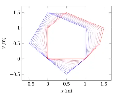
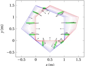
non-monotonous the morphing is. . . 43 3.7 Stability 2D polygon morphing: Ps in blue, Pd in red, the green and

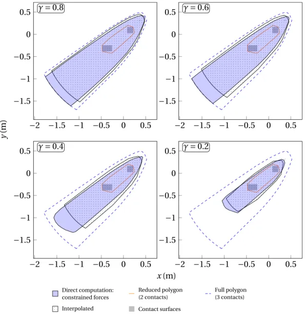
black arrows show the motion and the normals directions of the edges respectively. . . 45 3.8 Comparison between direct computation of the constrained static

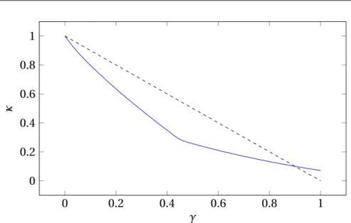
sta-bility polygon and interpolation. . . 46 3.9 Interpolation coefficient as a function of the force constraint coefficient

for a 3-contact scenario. Dashed line represents κ = 1 − γ. . . . 47 3.10 Climbing the stairs with HRP-2 Kai: with neither the constraint nor

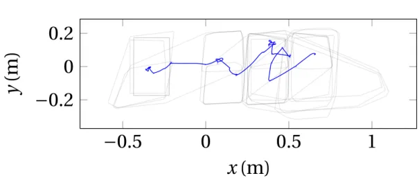
gripper torque task activated (left), with only the task (middle) and with both (right) . . . 51 3.11 In blue, the CoM trajectory during the experiment. In transparent grey,

the successive static stability polygons. The CoM notably interacts with the constraint at around (−0.25,0) and (0.5,0.05). . . 52 3.12 Still frames of HRP2 successfully climbing the stairs using the handrail.

(15)

3.13 Force (magnitude) applied on left hand during stairs climbing. Data was low-pass filetred by an order 2, Butterworth filter with a critical fre-quency of 10Hz. For phases, a,m,r stand for “add”, “move” and “remove” respectively while R,L,F,H stand for “Right”, “Left”, “Foot”, “Hand”. . . . 54 3.14 Snapshots of the force control experiment with HRP-2 to smoothly

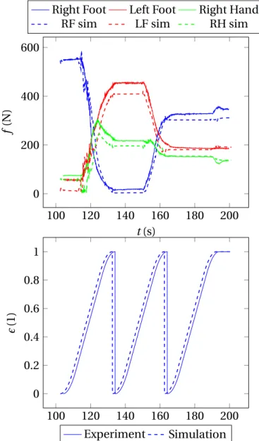
re-move the right foot. The CoM is smoothly pushed forward by the shrink-ing of the stability region, while the foot itself is admittance-controlled. No force distribution between the hand and left hand is given. . . 55 3.15 Results of multi-contact experiment and simulation. Top: normal force

applied on all contacts during motion. Bottom: interpolation index. . . 56 4.1 Illustration of the problem annotated with the variables. We propose

algorithms to compute the robust static stability P for the CoM c, know-ing the space G of the CoM’s accelerations ¨c. Individual contact forces are not named here. Instead, we only consider the set of all contact forces, denoted f . Contact surfaces are represented by green disks with the contact points and their normals, represented by the blue friction cones. p is the static stability polygon as computed in [Bretl and Lall, 2008]. . . 60 4.2 One iteration of the algorithm. (a) Initial state: the outer approximation

is a tetrahedron (transparent red). The search direction is perpendicular to the base: the extremal blue point is found, while the intersection by the new plane forms the three green points. (b) The inner approximation is now the blue tetrahedron. (c) Exploded view of the final state. The red tetrahedron is now outside of the outer approximation. The inner tetrahedron’s facets form three prismatoids with intersecting trapezoidal bases (thick orange, thin green, and transparent grey) by cutting the remaining outer approximation. . . 67 4.3 The robust static stability polyhedron as an intersection of oblique

prisms, for a residual radius gm= 3.55ms−2while the acceleration enve-lope is defined by G = {±gm,±gm, g }. . . . 73 4.4 Comparison of different P for different acceleration polytopes G

gener-ated by gm. Only the inner approximations Pinnerare rendered (in red),

but are almost superimposed with Pouter. The black dots with yellow

cones represent contact points with associated friction cones. . . 74 4.5 Comparison of different P for different acceleration spheres of radius

r . Only the inner approximations Pinnerare rendered (in red), but are

almost superimposed with Pouter. The black dots with yellow cones

(16)

List of Figures

4.6 Stability polygon in 2D (in red). The black dots with yellow cones repre-sent contact points with associated friction cones. . . 74 4.7 Computation times for 3 contacts, polytope with 4 vertices and 3 point

contacts. 50 iterations, total time 1.29s (clock time, without interpreter set-up and teardown). Final error: 0.043 m3. . . 75 4.8 Comparison between the convex hull of sampled points and the

com-puted P at various residual radiuses for different number of vertices of G . Sampled points were tested for stability with_{|G | = 18 . . . .} 77 4.9 Precision reached as a function of the number of iterations while

ap-proximating a sphere. . . 78 4.10 Number of iterations required to test random points compared to naive

sampling. The blue line represents the average number of iterations, the shaded area corresponds to the mininimum-maximum envelope. The red line represents the naive sampling: one iteration per query. The dashed lines reprensent the number of iterations necessary to reach the indicated precision using algorithm 3. . . 81 4.11 Morphing between two different robust static stability polyhedrons. . . 82 4.12 Comparison of morphing with direct computation for different keypoints. 84 4.13 Comparison between: the statically stable prism in light blue, the robust

static polyhedron with a G generated using gm = 2.6ms−2 in red and the prism formed by the robust polygon at the same margin and height 0.1 m in dark blue. Note that the scale is non-uniform across axes. . . . 85 4.14 Compare 2D robust and 3D robust at different heights (in meters).

Dashed lines represent volumes error, while solid lines represent ar-eas error. . . 86 4.15 Results obtained using posture generation. From left to right, both feet,

feet and right forearm, left foot and right forearm, each pair is first non-robust, labelled S, then non-robust, labelled R. The same robust polyhedron is displayed in both images of each pair. . . 87 4.16 Illustration of the inequality morphing from P0(dashed) to P1

(dot-dashed). The intermediate dilatations are in solid black. The interpolate at κ is filled in transparent red. . . . 89 4.17 Climbing the stairs under robust static stability constraints. In this

scenario, the weight of the CoM task is set to the lowest possible, 10. The current interpolate of the polyhedron is depicted in transparent green. Note how the robot tilts backwards: the CoM is only pushed forward by the constraint. . . 92 5.1 HRP-2 leaning: representation of variables used in modeling. . . 99 5.2 Data flow for MPC . . . 103

(17)

5.3 Multi-contact motion planning architecture. . . 106 5.4 HRP-2 going over a ridge: contact stances and transitions are illustrated. 111 5.5 HRP-2 Walking on uneven ground while carrying an object. . . 112 5.6 Uncontrolled momentum derivative ˙Lzcomputed on the whole-body

model (thin red) and reduced model (thick grey) with superposition of computed trajectories (multicolor transparent) . . . 113 5.7 Schema of the polyhedron CoM preview control. Left shows the

spa-tial trajectory going through three different polygons. Right shows the evolution of the integer variable with time. . . 114 5.8 Keyframes of HRP2-Kai crossing a ridge: the blue ribbon represents the

current CoM trajectory being tracked. . . 118 5.9 Keyframes of HRP2-Kai climbing the stairs: the blue ribbon represents

(18)

List of Tables

4.1 Computation time of 50 SOCP problems when considering a spherical G compared to the linearization. In the latter case, it is a function of the number of vertices of G . . . 76 4.2 Influence of the CoM task weight on success of stairs climbing, with and

without the polyhedral constraint activated . . . 92 5.1 Weights and Stiffness used in CoM Preview . . . 110

(19)

(20)

Introduction

The overarching theme of this thesis is to generate stable motion for legged robots, particularly humanoids. Those robots have the great advantage of being able to perform multi-contact motion: they can use a number of support points on the environment with any potential part of their bodies. They can thus theoretically walk, climb, crawl... while potentially carrying payloads. Yet, they have a fundamental defect compared to fixed platforms: they can loose balance and fall. This problem makes them unreliable, and it is what prevents them from being widely used.

In the industry, robots have been everywhere for decades: most of them are fixed arms, operating at high speeds, and performing high-precision tasks. Those robots must interact with the physical world and manipulate heavy payloads. However they do so without having to consider stability: even when perturbed, there is no way they will not be able to resume operation short of mechanical failure. The other categories of robots that are currently at the center of commercial projects are autonomous cars and drones. The former are inherently stable, the latter can freely move in space without contact.

Nowadays, most homes are equipped with a robotic solution. The most popular home “robotics” applications remain focused on artificial intelligence and are mainly tasked with speech and image recognition. However a close contender are a domotic solutions: a wheeled robot, that performs vacuuming, lawn mowing, pool cleaning, etc. They are naturally stable due to their structure: they all present a large base and are very short. This ensures their stability, especially on flat terrains. Another category of robots is spreading in homes: toys. Whether light remote controlled drones, boats, or spherical robots, they do not need to properly consider stability. Moreover, they present a low number of degrees of freedom.

Finally, service robots are starting to appear and serve as guides, receptionists, and personal assistants. They are often composed of a wheeled base surmounted by an humanoid torso. As they are top-heavy, their stability is not guaranteed but is controlled by properly accelerating the base. Yet, they are not designed to handle

(21)

physical contact, and cannot lift heavy charges.

Thus technologies more recently adopted are closer to humanoid robotics, and require more advanced notions of stability. Yet, an important range of applications is not addressed by those platforms:

• Locomotion across rough terrains, including stairs, ladders and narrow catwalks. • Manipulation of heavy payloads in an unstructured environment.

Those scenarios will typically arise in disaster recovery scenarios, as evidenced by the Darpa Robotics Challenge1, where a robot will typically have to cross rough terrain, clear heavy debris to access an objective, typically a switch, valve or control panel. However, those use cases are not only exceptional, but an everyday occurrence in manufacturing scenarios. Indeed, on construction sites, in shipyards and in airplane assembly factories, the only way to get around is on foot, as there are no ramps to change floors, and the floor itself is often not complete. Finally, in those places it is very important to be robust to external perturbations as the robot will interact not only with unstructured terrain but humans.

To generate robotic motion, most approaches so far have either considered one of two options:

• Generating stable keyframes and interpolating between them. This interpo-lation generally does not guarantee stability, which means that the motion is often hand-tuned to obtain a satisfying result.

• Generating a stable trajectory. Note that as the trajectory is often composed of a finite number of waypoints, a similar problem to the above point is raised. However, those waypoints are usually very close to one another, which makes the assumption of stability in between them more reasonable.

Yet, in both cases, no notion of stable affordances was introduced: the generated motion could be only marginally stable. This means that any outside perturbation, or any error in the execution (due to imperfect actuation) could lead to falling.

Hence, in this thesis we will generate motion that is not only stable on a point-to-point basis, but that is constrained to a known region of stability. We will also introduce the notion of affordances that will give us a region of robust stability. As those regions are

(22)

projections of high-dimensional convex bodies defined by inequalities, obtaining their explicit representation requires a special set of tools and algorithms to be computed efficiently. Thus, we focus on developing new algorithms to compute those regions and to use them within a multi-contact control framework.

The first chapter of this thesis thus presents the basis of the notion of stability, or equi-librium. Starting from the equations of motion, we show that they are not sufficient to properly discriminate between stable and unstable motion. As this notion is central to the field of legged robotics, we also present the relevant prior work and introduce our ideas.

In the second chapter, we recall some well-known mathematical notions that are central to this thesis.

In the third chapter, we show that we can compute a region of static equilibrium, that is to say a set of acceptable positions supposing that the robot is not moving. This region can be deformed according to the set of acceptable contact forces: this prove to be useful to determine how to move the robot in order to obtain the desired contact force. Moreover, we introduce computer graphics algorithms that continuously deform this region. Finally, this deformable region is integrated in our control framework, and the results evaluated on a real hardware.

In the fourth chapter, we show that introducing the notion of stability affordances results in a substantial increase of complexity: whereas the static equilibrium region is a right prism whose base can be computed in 2 dimensions, the robust static

equilibrium region is a general 3-dimensional shape. We show the different ways to

compute this shape, and, similarly to the previous chapter, which algorithms can be used to continuously deform it. This can be used for scaling up or down the affordances and for multi-contact control.

Finally, the fifth chapter introduces two different, yet related, methods to perform multi-contact trajectory generation. The first one is a general method to perform multi-contact motion that takes advantage of the whole dynamics of the robot. The second one is based on the notion of robust static equilibrium: it is very efficient in terms of computation time but does not exploit the full extent of the robot dynamics. However, as it includes a notion of affordances, it can be seen as safer in the sense that it is resilient to perturbations.

Finally, we conclude our work and present some ideas for extensions and future works. Enhancements of both a technical and theoretical nature are discussed together with new applications.

(23)

In the next chapter, we review the state of the art and contrast it to the works presented in this thesis.

(24)

1 State of the Art

Stability is of prime importance for legged robots, and in particular humanoid robots. As they are under-actuated systems, it is important to retain controlability of the non-actuated floating base. Indeed, a fall is a failure that can cause serious dam-age to the robot’s structure. Even if some promising approaches are currently re-searched to limit the damage received during a fall [Samy and Kheddar, 2015] and to autonomously stand back up [Fujiwara et al., 2003], they are not sufficient to make falling safe. Moreover, in industrial scenarios, such as those envisioned in the Darpa Robotics Challenge1, falling can have catastrophic, non-recoverable consequences, especially if falling from a great height or into sharp debris. Similarly, the European research project COMANOID2aims at performing multi-contact motion inside an in-construction airplane. Falling would damage the airplane, and is unnaceptable. Thus, the notion of stability has been extensively studied throughout the years, and many different approaches have shed light on how to retain control of a moving legged robot.

To better understand the mathematical challenges underlying stability, let us go back to the rigid-body dynamics that describes the evolution of the robot’s state as it interacts with its environment.

H(q) ¨q +C(q, ˙q) ˙q + g(q) = J(q)Tf + τ (1.1)

This equation shows us that joint accelerations are linked in a non-linear fashion to contact forces, torques and the non-linear Coriolis and gravity terms [Featherstone,

1_{http://archive.darpa.mil/roboticschallenge/} 2_{http://comanoid.cnrs.fr/}

(25)

2008]. By adding a Coulomb friction cone constraint, we can construct a full model of the robot’s motion:

° °B f

°

°≤ uTf (1.2)

This form can be considered locally linear in ¨q and f , that is to say, if we consider q

and ˙q to be constants as well as discretizing the friction cones. Making this constraint

linear makes it easy to use it in a convex optimization program, such as a quadratic program (QP), without any simplifcation of the robot model. This kind of programs are very fast to solve, in the order of a millisecond for about a hundred variables, making it a great tool to be used in real-time, whole-body, multi-contact applications. This quasi-static interpretation is at the heart of most tasks-based controllers. Some are strictly prioritized task-space controllers [Sentis et al., 2010, Saab et al., 2012]. Others are weighted task-space controllers [Collette et al., 2007, Salini et al., 2010, Ott et al., 2011, Bouyarmane and Kheddar, 2011a, Righetti et al., 2013, Vaillant et al., 2016]. Both approaches are similar, and only slightly differ in capabilities. Although, controller robustness depends heavily on the numerical solver they use (generally off-the-shelf [Gill et al., 1986, Turlach, 1998] or customized [Escande et al., 2014] QP solvers), they were used with great success in a variety of scenarios. Indeed, some of the best performing teams at DRC used such an approach [Feng et al., 2014, Kuindersma et al., 2015, Koolen et al., 2016] as part of their control pipeline in order to perform egress/ingress from a car. Other works [Bouyarmane and Kheddar, 2012, Vaillant et al., 2016] exploited with success such approaches to access confined spaces in more complex scenarios.

However, this approach has many limitations, the main one being that it does not directly prevent the robot from falling. Indeed, setting ˙q, f and τ to zero gives us

a perfectly acceptable solution where the robot accelerates in the gravity field, i.e. free falls. This problem can become very acute when using the above quasi-static approach: if the robot ventures in an area where the only solution is falling, it is unlikely that it will be able to correct its course. In that sense falling is an attractor of the motion, albeit an undesirable one and Equation 1.1 does not describe stability but rather the notion of compatibility, that is to say, is an oracle to tell us if some contact forces are coherent with some joint accelerations in a given robot state.

A second issue is that transitions between contacts is a discrete event, that cannot be captured by local regulation schemes. Indeed, transitioning between contacts requires modifying the force distribution, but (1.1) is not sufficient to judge the feasibility of a force distribution.

(26)

1.1. Using a stronger stability criterion

To tackle these problems, most solutions fall into one of two categories:

• Instead of using general dynamic stability, use a stronger local stability criterion that will reject falling as an unacceptable solution.

• Instead of only considering the local time, look for a solution over a time horizon. This will automatically reject the falling trajectories as they will come with a high cost: it is in general impossible to follow a given objective while falling.

Of course, some solutions may use both. We will see in the following sections that using reduced models leads to great improvements in computation times. This fact can be exploited for real-time operation or for computing more than one solution, sometimes all solutions, in the alloted time.

1.1 Using a stronger stability criterion

In order to smoothly transition between contacts, we want to specify only a desired force profile on a given contact without endangering stability.

Whole body controllers typically solve an optimization problem that aims at finding compatible joint accelerations, ¨q and contact forces λ by minimizing a set of task

errors under constraints. Stability is typically enforced by controlling the position of the Center of Mass, or a derived quantity.

On the one hand, the current frameworks can not handle an unified force - stability objective. Indeed, let us consider a general stability objective that depends on the generalized coordinates and their derivatives, q, ˙q, ¨q and the contact forces f . Then,

we will see in chapter 2 that typical frameworks transform this general task error X into a quadratic objective FX in ¨q and f . However, this is not possible in our case, as one must differentiate the general objective with respect to time. This would entail derivating f , but f are part of our optimization variables.

On the other hand, separate objectives require carefully setting each objective:

• A task to minimize the 2-norm of λ will not result in modification of angular values: the best local solution is redistributing the internal torques to fall as little as possible.

• Controlling the CoM will require to set gains that will interfere with almost all the other tasks, such as end-effectors trajectories.

(27)

This is why several works [Ott et al., 2011, Lee and Goswami, 2012, Righetti et al., 2013, Herzog et al., 2014] have proposed efficient force regulation control strategies in multi-contact configurations, but in all of those cases, the CoM was regulated independently.

Instead of considering the whole dynamics, we can employ a stronger stability criteria that will lead to simpler, faster, computations.

A very well known reduced-model criterion is the Zero-Moment Point. The original ZMP criterion [Vukobratovi´c and Borovac, 2004] is the extension of the convex hull

criterion and has been widely used in biped locomotion on flat grounds assuming high

friction, e.g. [Kajita et al., 2003]. Unfortunately, it is only applicable for locomotion on flat ground and does not take friction into account. The ZMP is better defined in [Goswami, 1999], and its similarity to the Center of Pressure (CoP) is highlighted in [Sardain and Bessonnet, 2004].

One can enforce stability in multi-contact by controlling the Center of Pressure (CoP) at each contact to remain within the convex hull of its area [Sentis et al., 2010, Righetti et al., 2013, Herzog et al., 2014, Audren et al., 2014, Feng et al., 2014, Hyon and Cheng, 2007, Wensing et al., 2013, Nori et al., 2015]. This strategy similarly requires controlling the contact forces. In these implementations, the CoM objective was given as a high-level task, and the CoP or contact forces were regulated in the null-space or in conjunction with the CoM task. Yet, the CoP is not defined when the normal force applied on the contact is nil, and is not easily extensible to bilateral contacts.

Thus let us consider an even simpler criterion: static stability [McGhee and Frank, 1968]. We rewrite the whole-body problem (1.1) as:

g (q) = J(q)Tf + τ (1.3)

While keeping the Coulomb friction constraint (1.2). This allows us to characterize all postures that are undefinitely (in terms of time) sustainable by the robot being considered. However, this entirely disregards the dynamics of the motion.

Using this formulation, one can formulate a non-linear optimization problem in q and

f that will aim at finding compatible joint angles (including free-flyer position) and

contact forces [Escande et al., 2013, Brossette et al., 2015, Bouyarmane and Kheddar, 2012, Brossette et al., 2016]. Such a problem is often referred to as posture generation. However, keeping such a non-linear formulations requires an expensive optimization process to be run to find one solution, making it ill-adapted at real-time applications,

(28)

1.2. Going further than locally

but a perfect match for offline planning applications. Indeed, it does not simplify the kinematics, can be refined to include constraints such as joint limits, torque limits, and will automatically find the position of the contacts.

Yet, to actually perform the motion, one needs to design a controller that will allow to move from one planned stance to the next. In general, stability is not guaranteed in-between the stances, and even basic feasibility is not granted.

Thus, we want to find a region of stability inside which stability is guaranteed. Remain-ing in this region would be a hard constraint. We can then add a CoM objective among the tasks to be achieved at best with a low priority to guide the controller towards a particular solution.

We have shown in [Audren et al., 2016] and chapter 3 that static stability can be leveraged, for complex multi-contact motion because it is easy to find every statically stable position of the CoM given a set of contacts. Indeed, at least three techniques are available to compute the region of static stability: direct projection based on double-description [Fukuda and Prodon, 1996a], recursive projection [Bretl and Lall, 2008] and a quasi-analytic formulation [Or and Rimon, 2016]. We will moreover show that the computation of this set of positions depends on the allowed contact forces, and can be leveraged to perform multi-contact force regulation. It is then a matter of designing a controller that can enforce the correct constraints.

1.2 Going further than locally

One usual way to circumvent the local-view issue is to use a preview controller to enhance the motion with a flavor of dynamics [Audren et al., 2014, Dai et al., 2014], but slow multi-contact motion can be achieved without preview [Vaillant et al., 2016], using only a closed-loop local task-based controller.

Trajectory optimization is a very rich field, that provides the ability to look ahead, and find a solution that is not only locally optimal, but a motion that is optimal over a time interval. This enforces stability by making sure that we reach a goal: if the robot fell midway, it will never reach the desired target. However, generic trajectory optimization remains a slow process. The most general methods do not make any assumptions on the model nor the motion, but can be very slow to optimize a whole-body trajectory [Lengagne et al., 2013, Kudruss et al., 2015, Posa et al., 2014], on the order of several minutes to reach a solution.

(29)

Hauser, 2014] on a single core. Even approaches that leverage the high-parallelism ca-pabilities of Graphic Processing Units (GPU) cannot keep up with real-time [Chrétien et al., 2016].

Although well-suited for planning, those approaches are not reactive. Indeed, the longer the trajectory optimization process takes, the slower the robot will respond to external perturbations. A very popular technique to compensate for perturbations of the current state while taking into account its repercussions into the future is Model Predictive Control (MPC) also known as Model Preview Control or also as Receding Horizon Control.

Appearing about 30 years ago [Clarke et al., 1987] for industrial plant control applica-tions, the technique aims at finding control inputs over a time horizon that minimize an objective function based on the output of the plant model. The model is thus inherently recursive, as successive control inputs will affect the rest of the preview horizon: state feedback is taken into account over the whole horizon. This also gives the opportunity to compensate for modelling errors: if the preview horizon is chosen to be much larger than the computation time, only the beginning of the trajectory will be used. The next optimization will start from the current state, which will differ from the model-based prediction of the plant state.

In robotics, time scales are generally short (from the millisecond to the second) while industrial plant applications operate on a larger scale (from the second to the week). Thus, careful selection of the predictive model is essential to make sure that recom-putation of the preview control can happen in time. One of the most well-known application of predictive control is ZMP preview control [Kajita et al., 2003] for hu-manoid bipedal locomotion. In that case, the reduced model used for predictive modelling is a very simple cart-table model: the robot is assimilated to a single rigid body (the cart) that can only move in a plane of fixed height (the table). This allows for linear formulation of the ZMP dynamics, and thus for very fast resolution, by reducing to an unconstrained Linear Quadratic Regulator problem. A whole-body controller based on Inverse Kinematics (IK) is then applied to track the generated ZMP trajectory. This application set a high performance standard even if it entirely neglects friction constraints, is only applicable to flat ground locomotion, and necessitates as input a target ZMP trajectory.

Since then, the area of predictive control strives to solve more general problems. Using a more complex model, the Spring-Loaded Inverted Pendulum (SLIP), [Mordatch et al., 2010] used this approach to realize more challenging motion and various gaits, from walking to running with full-flight phases. However, this approach was still limited to walking applications and was not real-time, due to the underlying whole-body

(30)

1.3. Handling the non-linearity

controller.

To further improve the performance of such a controller, [Ibanez et al., 2014] proposed to extend the state with a set of integer variables that allow for discrete decision making. This controller is able to automatically choose the position of the feet which allows to choose a gait in reaction to changes in desired velocity and external disturbances. Then, in our work [Audren et al., 2014] that we will elaborate on in chapter 5 we propose a CoM preview-control formulation to extend this formalism to multi-contact locomotion, that takes into account contact friction. It relies on reducing the robot to a freewheel model, that is to say a single body with mass and inertia, located at the center of mass. Then by solving an optimization problem on the CoM acceleration and contact forces, considered as the command inputs, we are able to generate 3-dimensional trajectories. However, this solution is limited by the necessity to fix the acceleration of the CoM in a particular direction and results in uncontrolled momentum over one axis.

Even when the whole-body dynamics is reduced to its center-of-mass [Orin et al., 2013, Audren et al., 2014], the resulting equations exhibit the angular momentum of the body as a cross-product between the contact forces and the CoM position; an operation that is neither linear nor convex:

¨c =X i fi (1.4) ˙L = X i fi× (c − pi) (1.5)

To avoid this, two approaches remain: go back to a simpler, but stricly stronger criterion, or try to deal with this non-linearity head-on.

1.3 Handling the non-linearity

Going back to preview control, it would be interesting to design three dimensional, unconstrained trajectories. However, one needs to take a particular approach to handle the non-linearity that appears when considering the dynamics of the flywheel model.

Some approaches solve head-on the non-linear problem, for example [Caron and Kheddar, 2017]. Specialized optimization techniques are employed to make the

(31)

reso-lution very fast [Serra et al., 2016].

To do so, [Herzog et al., 2015] propose to solve the momentum non-linear dynamics head-on by using a dynamic programming scheme but lose the real-time capabilities of the system as they need several passes of quadratic programming and inverse kinematics to reach their goal. In later works [Herzog et al., 2016], the authors modify their approach to better isolate non-linearity of the problem at the cost of increased complexity in the constraints, turning it into a Quadratically Constrained Quadratic Program (QCQP) but in doing so highly reduce the complexity class of their problem, rendering it linear in the number of timesteps. Now, they have developped a convex approximation of the dynamics [Ponton et al., 2016], by approximating the non-convex quadratic constraint part by a difference of convex functions.

Another solution is to decouple the acceleration from the contact forces. By restricting either the center of mass acceleration or position to lie within a convex polytope, one can compute the convex envelope of the other.

Our idea is to compute a hull P for the CoM, such that ∀ CoM ∈ P , the stability is guaranteed to be robust w.r.t to a given set of accelerations G . That is to say, for all possible CoM positions that lie within P and, there exist a set of contact forces that can generate any acceleration in G . In other words, we compute the intersection of G with the set of all possible motions. We show that this intersection results in a convex volume that we project in the CoM space. Hence, by defining G , the CoM acceleration and its position are decoupled. Other restrictions can been set to obtain such a decoupling. One of the most stringent is to set the CoM acceleration to zero, resulting in the static stability criterion as in the previous section.

Static stability can be expressed as a function of the gravity orientation. Indeed [Mat-tikalli et al., 1996, Mosemann et al., 1997] present a way to find all the gravity ori-entations that satisfy static stability of assemblies: it is a convex region defined by inequalities. They apply early vertex enumeration techniques —that we also use, to compute the acceptable region. Yet, the objects were fixed and not actuated.

The next step was to extend the idea of the ZMP and convex hull to multi-contact motion. This gave us a new criteria: the resultant wrench of the contact forces must remain in a polyhedral convex cone. Pioneered by [Saida et al., 2003], it formed the basis of the work in [Hirukawa et al., 2006] ostensibly titled “Adios ZMP”. It is applicable to multi-contact motion while remaining linear and global. This criterion is more clearly and properly established and applied to multi-contact motion in [Caron et al., 2015, Caron et al., 2017]. In the latter works, a new ZMP-like criterion (a pseudo-ZMP) that has to remain in the two-dimensional projection of the convex polyhedral wrench

(32)

1.3. Handling the non-linearity

cone is proposed. It is applicable to multi-contact motion and takes into account friction. Note that, similarly to the ZMP and the CoP, the pseudo-ZMP support area depends on the instantaneous CoM position.

Constraining the CoM to remain in the static stability polygon p is a global, CoM based, and linear criterion. Unfortunately, static stability (equilibrium) criterion does not imply dynamic stability [Garcia et al., 2002, Audren et al., 2016]. Indeed tracking a statically stable trajectory with changes in acceleration may induce falling. Thus, static stability is marginal, i.e. not robust to changes in the total acceleration.

Instead, our approach, presented in chapter 4 imposes constraints on the resultant acceleration and finds a linear, global corresponding constraint on the CoM. It the natural extension of the previous chapter chapter 3: instead of computing regular static stability regions, we add explicit stability margins.

We propose algorithms to compute a robust stability region P for a given G . This decoupling will be exploited in a MPC formulation in chapter 5.

In what can be seen as the dual of our approach, restricting the CoM position results in the volume of accelerations being an intersection of cones, as presented in [Caron and Kheddar, 2016].

Note that other non-linearities arise when allowing more parameters to vary: the timing of steps, as in [Ibanez et al., 2014], but also the position of the contacts [Deits and Tedrake, 2015, Kuindersma et al., 2015]. In both cases, using integer variables to change between discrete values allows to keep the problem linear. For timings, another approach is to first (linearly) compute an acceptable trajectory over the contacts, and then compute a Time Optimal Path Parametrization [Pham, 2014] to obtain the timings of the change in contacts [Caron and Pham, 2016, Hauser, 2014].

(33)

(34)

2 Preliminaries

Before delving into the contributions of this thesis, important building blocks have to be presented:

• Optimization, and a few typical programs as a way to find numerical solutions to generic problems.

• Posture generation as a tool to generate key postures and to find contacts.

• Task-based inverse dynamics to perform whole-body control.

2.1 Optimization

Optimization is a field of mathematics that is concerned with minimizing a certain function, called the objective or the cost function. The input is thus a function, f :

F :E7→ R (2.1)

x 7→ F (x)

And the output is a x∗_{such that:}

F (x∗) = min

x∈E F (x) (2.2)

(35)

is denoted in short hand as:

min.

x F (x) (2.3)

As x can take any value in E, the above problem is an instance of an unconstrained program. In the general case, the acceptable values of x will be restricted through the use of constraints: min. x F (x) (2.4) s.t. l ≤ C (x) ≤ u Where C is a function: C :E_{7→ R}n (2.5) x 7→ C (x) (2.6)

And l, u are vectors inRn_{that represent the bounds on C . If there exists a x ∈ E such} that l ≤ C (x) ≤ u, then the problem is said to be feasible.

If F and C have analytical expressions, it might be possible to analytically derive the optimal value of the optimization problem. However, most often, we can only numeri-cally compute the value of the objective and constraints, as well as their derivatives: we will solve numerical optimization problems.

If F and C have no specific form over E = Rn_{, we will refer to the problem they form} as a non-linear optimization problem. If F is a quadratic function i.e. if there exists a positive semi-definite matrix Q and a vector v such that:

∀x ∈ Rn, F (x) =1 2x

T_{Qx + v}T_x _(2.7)

And if C is a linear function, i.e. there exists a matrix A such that:

(36)

2.2. Posture Generation

Then the program:

min. x 1 2x T_{Qx + c}T_x _(2.9) s.t. l ≤ Ax ≤ u (2.10)

Is said to be a quadratic program.

If F is a linear function, i.e. if there exists a vector v inRn_{such that:}

∀x ∈ E, F (x) = vTx (2.11)

And C represents l2cones i.e. there exists a sequence of matrices Ai, vectors bi and

vi: C (x)₌     kA0x + b0k2− v₀Tx .. . kAnk + bkk2− vkTx     (2.12)

Then this optimization problem is a second-order cone program, SOCP in short-hand. Note that if F is convex, it has only one global minimum, whereas a general F can present many local minima. Thus if F and C are convex (i.e. F is a convex function over a convex set), the problem is said to be a convex optimization problem. It can generally be solved faster than generic problems, and the solution is guaranteed to be globally optimal. For more details on how to solve such programs, refer to e.g. [Boyd and Vandenberghe, 2004].

2.2 Posture Generation

Posture generation (PG) in the context of legged robotics consists in finding a robot

posture: it is a generalized inverse kinematics problem. Indeed, solving a PG problem

not only results in a set of generalized coordinates q but also in a set of contact forces

f that satisfies a set of constraints. Those constraints typically comprise:

• Contact constraints: the contact forces f can only be applied at points where the robot’s body touches the environment. Moreover, they must obey Coulomb’s friction law.

(37)

within their limits, and the resulting momentum at the center of mass must be null.

• Collision constraints: they prevent self-intersection and undesirable contacts with the environment.

• Joint limits: the joint angles q must remain within their acceptable range.

The objective function can be varied, but will often encode:

• Distance to a usual posture • Force distribution on contacts

• Specific bodies orientation or position

Finding such a set q, f can be reduced to solving a non-linear optimization problem, possibly over non-euclidian manifolds [Escande et al., 2013, Brossette et al., 2015, Brossette et al., 2016]. Indeed rotations live in the special orthogonal group and not in an euclidian space.

Due to its non-linear nature, and because a humanoid robot has a high number of degrees of freedom, solving a PG problem cannot be done in real-time: it takes around a second to do so whereas the robot control loop runs at around 500 Hz. Moreover, posture generation is static by nature, and thus cannot be used to generate motion. The next section will present a generic approach to do so.

2.3 Task-based inverse dynamics

Task-based inverse dynamics, or tasks-based controller, or also QP controllers aim at finding optimal accelerations to realize certain tasks under constraints. They are most often formalized as a QP over the joint accelerations ¨q and contact forces f . The

QP formulation allows to formulate objectives in terms of distance (in the sense of

l2norm) but does not compromise performance. Indeed, the programs presented below can be solved in the order of the millisecond by off-the-shelf solvers [Gill et al., 1986, Turlach, 1998].

The first constraint of any motion is of course dynamic compatibility. Rigid body dynamics, as presented in (1.1) can be considered linear in ¨q, f ,τ: this is true if and

(38)

2.3. Task-based inverse dynamics

amount to consider small accelerations ¨q. In discrete time, it amounts to assuming

that q, ˙q is constant over one timestep. In both cases, it means that variations of q, ¨q

are slow with respect to the time period.

Then, the Coulomb friction constraint (1.2) can also be linearized by considering poly-hedral cones instead of l2cones. To do so, a possible parametrization is to consider a new set of variables, λ that represent the force intensity along each generator of the polyhedral cones. Thus,

f = Nλ (2.13)

is guaranteed to be inside the polyhedral cone iff:

λ_{≥ 0} (2.14)

We also need to consider torque limits:

τl≤ τ ≤ τu (2.15)

This can be used to eliminate the τ variable, and form the motion constraints of our problem:

τ_l_{≤ H(q) ¨q +C(q, ˙q) ˙q + g (q) − J(q)}T_{N λ ≤ τ}u (2.16)

0 ≤ λ (2.17)

We now need to form additional constraints and objectives: those will often be speci-fied in the operational space. Thus, the task can be specispeci-fied by:

• A reference Xd, and eventually a speed reference ˙Xdand an acceleration refer-ence ¨Xd.

• A non-linear function X (q), its jacobian (derivative w.r.t q) JX and ˙JX.

The objective is to make X (q) converge to Xd. Because X does not depend on ¨q and because it is non-linear, it cannot be used directly in our QP objective. To transform it,

(39)

we first reveal the dependency to ¨q by deriving twice the error:

²_{= X}d− X (q) (2.18)

˙² = ˙Xd− JXq˙ (2.19)

¨² = ¨Xd− ˙JXq − J˙ Xq¨ (2.20)

We then implement a task-space proportional derivative control: finding ¨q that

mini-mizes: FX=°°Kp²− K_d˙²− ¨² ° ° 2 (2.21)

Will bring X to Xd without violating constraints.

Note that FX is a quadratic function in ¨q and is suitable for a QP objective. To combine different objectives, we use a weighted average: instead of minimizing a single FX, we consider a set of FXi and corresponding positive weights wi:

F =X wiFXi (2.22)

The same definition of ² can be used in inequality constraints: suppose that we want to enforce X (q) ≥ Xd. Then, by ensuring that:

˙

X (q) ≥ 0 (2.23)

we will ensure that X is increasing, and thus stay away from the bound. As we do not want to keep this constraint activated at all times, we only activate it under some interaction threshold ²i.

We use an integral formulation to ensure that ˙X is increasing at the next step:

JXq + dt ¡ ˙J˙ Xq + J˙ Xq¢ ≥ 0¨ (2.24)

To avoid strong discontinuities, we introduce a damping term ξ:

JXq + dt ¡ ˙J˙ Xq + J˙ Xq¢ − ξ(²) ≥ 0¨ (2.25)

The damping is a positive term, that is equal to 0 when ² = 0 and large when ² = ²i. We can then solve the optimization problem composed of a F defined by (2.22), a motion constraint of the form Equations (2.16) to (2.17), and possibly more constraints

(40)

2.3. Task-based inverse dynamics

of the form (2.25). This yields the optimal ¨q and λ. If the robot being considered

is torque-controlled, it is straightforward to reconstruct τ from ¨q and λ using (1.1).

Otherwise, if the robot is position controlled, integrating ¨q twice yields joint angles q

that are in turn fed to the joint-level controller of the robot.

The QP can then be solved at each timestep, and produce complete trajectories in real-time. For more details, see [de Lasa et al., 2010, Bouyarmane and Kheddar, 2012, Vaillant et al., 2016].

(41)

(42)

3 Static equilibrium and interpolation

As presented in chapter 1, we will study how static stability can be used in multi-contact control. This chapter presents three key aspects: computation of the static stability polygon, development of an optimal matching for interpolation and integra-tion with our multi-contact control framework. Finally, experimental results will be presented.

In this chapter, we will limit our developments to multi-contact, quasi-static motion. Hence, constraining the CoM to remain within the frictional static stability polygon is an acceptable criterion. Chapter 4 will extend this work to dynamic motion by taking into account acceleration of the Center of Mass.

Although computation of the static stability polygon is well-known, its dependency on the admissible contact forces has not extensively treated. Thus, we show in section 3.1 how the static stability polygon deforms as a function of the admissible forces, first on simple cases, then in the general case.

As we will integrate this CoM stability region as a hard constraint in our controller, it is necessary to avoid discontinuities. Indeed, if the constraint is not continuous, it might get suddenly violated, thus triggering a controller failure. To solve this problem, we introduce we introduce the notion of polygonal morphing in section 3.2. This technique, based on optimal matching, will allow us to approximate changes in the admissible contact forces (c.f. section 3.3).

Finally, section 3.4 will present how the previous points are used in our controller. In subsection 3.4.1 we present how to use the morphing as a constraint. Then we demonstrate how to climb stairs in subsection 3.4.2. We present a way to efficiently combine force control tasks with this constraint in subsection 3.4.4 and present results obtained in another multi-contact scenario in subsection 3.4.5.

(43)

3.1 Computation of the constrained stability polygon

In the typical case, the static stability region only depends on the geometrical and frictional properties of the contacts. How does this shape evolve as we restrict the admissible contact forces? We will first present simple examples in sections 3.1.1 to 3.1.4 before presenting generic algorithms in sections 3.1.5 and 3.1.6.

In each case, the region is naturally described by a set of inequalities and equalities in c and f . The goal is to find the extremal values of c. This amounts to a problem of

vertex enumeration. Indeed, a set of linear inequalities describes a convex polyhedron,

while a set of equalities amounts to projecting on a subspace. The question is thus: what are the vertices of this projection?

3.1.1 1D CoM - 2 aligned forces

We consider a 2D case with a robot whose coordinates are:

c =hcx czi (3.1)

It has two contact points with the environment, with their associated contact forces (expressed in the world frame):

p1= h p₁x 0i→ f1= h f₁z f₁xi (3.2) p2= h p₂x 0i_{→ f}2= h f₂z f₂xi (3.3)

The Newton-Euler equations are:

f1+ f2= mg (3.4)

(c − p1) × f1+ (c − p2) × f2= 0 (3.5)

As the contact points have vertical normals, the friction equations become:

|f1x| ≤ µf1z (3.6)

(44)

3.1. Computation of the constrained stability polygon

We then project every equation on every axis:

f₁x+ f2x= 0 (3.8) f₁z_{+ f}₂z_{= mg} (3.9) f₁xcz_{+ f}₂xcz_{= 0} (3.10) f₁z(cx− px1) + f2z(cx− p2x) = 0 (3.11) f₁x_{≤ µf}₁z (3.12) f₂x_{≤ µf}₂z (3.13) −f1x≤ µf1z (3.14) −f2x≤ µf2z (3.15)

We want to find the boundaries of cx, i.e. min(cx) and max(cx). Notice that f₁x_{= f}₂x_{= 0} satisfies all the equations in which they appear, and thus any value of czis acceptable. We reorganize (3.11) to isolate cx: cx(f₁z_{+ f}₂z) − p1xf1z− p2xf2z= 0 (3.16) cx= p x 1f1z+ px2f2z mg (3.17)

Thus x can only be the barycenter of p1and p2weighted by f₁zand f₂z. As f₁zand f₂z

are both positive and their sum is non-zero, we are sure that cx_∈£

px

1, p2x

¤

. If we limit the intensity of f₁zand f₂zto ¯f, we then have:

x ∈ ·_p 1¯f+p2(mg − ¯f) mg , p1(mg − ¯f) + p2¯f mg ¸ (3.18)

Indeed, there are only two ways to saturate the inequality constraints: either saturate

f₁zfirst and then f₂zor the converse. If ¯f < 0.5mg then there is no solution.

3.1.2 1D CoM - 2 non-aligned forces

We consider a slightly more general case: we keep the same model as in the previous section, but the contact normals are no longer vertical. We denote them n1and n2,

they respectively form an angle α1and α2with the horizontal. See section 3.1.2 for an

(45)

x y p1 p2 α₁ _α₂ f1 f2 CoM

Figure 3.1 Schema for two non-aligned contacts

In that case, the Newton-Euler equations remain the same:

f₁x_{+ f}₂x_{= 0} (3.19)

f₁z+ f2z= mg (3.20)

f₁xz + f2xz = 0 (3.21)

f₁z(cx_{− p}1) + f2z(cx− p2) = 0 (3.22)

And we can still deduce that:

cx₌ f

z

1p1+ f2zp2

mg (3.23)

But the Coulomb friction equations are more involved:

|sinα1f1z− cosα1f1x| ≤ µ ¡ sinα1f1x+ cosα1f1z ¢ (3.24) |sinα2f2z− cosα2f2x| ≤ µ ¡ sinα2f2x+ cosα2f2z ¢ (3.25)

Meaning that indeed, the CoM is still the barycenter of the contact points weighted by the vertical forces, but finding the maximum value for each force is not evident. We can remove the absolute value by considering both options:

sinα1f₁z− cosα1f₁x≤ µ¡sinα1f₁x+ cosα1f₁z¢ (3.26)

−sinα1f1z+ cosα1f1x≤ µ

¡

sinα1f1x+ cosα1f1z

¢

(46)

3.1. Computation of the constrained stability polygon

And similarly for f2. This can be rewritten in shorthand:

f₁xa1+ f1zb1≥ 0 (3.28)

f₁xc1+ f1zd1≥ 0 (3.29)

By using the two last lines of Euler-Newton we can reduce it to a set of four inequalities in two variables, f₁z, f₁x:

f₁xa1+ f1zb1≥ 0 (3.30)

f₁xc1+ f1zd1≥ 0 (3.31)

−f1xa2+ (mg − f1z)b2≥ 0 (3.32)

−f1xc2+ (mg − f1z)d2≥ 0 (3.33)

We can plot this in the f₁x, f₁zspace, see section 3.1.2. It highlights the fact that the interval we look has basically two forms: if g is in the friction cones, it is £px₁, px₂¤ . Otherwise, it is a much smaller interval, that is hard to determine analytically. Indeed, the combinatoriality of the above system cannot be reduced: one has to make assump-tions to deduce an actual bound. Supposing that all of the inequality coefficients are strictly positive and thatb1a2

a1b2 > 1, d1a2 c1b2 > 1, b1c2 a1d2 > 1, d1c2 c1d2> 1 the bound on f z 1 is: f₁z_{≤ min(} mg a1 a1b2− b1a2, mg c1 c1b2− d1a2, mg a1 a1d2− b1c2, mg c1 c1d2− d1c2) (3.34) 400 200 0 200 400 400 200 0 200 400 12 3 4

Figure 3.2 Plot of the inequalities with highlighted intersection points. The left plot was realized with α1= 0.4,α2= 0.4 while the right one uses α1= 0.5,α2= 0.4. Dashed

lines represent ±mg. arctanµ ≈ 0.46

Then, to find the range of possible cx, one has to find the intersection of the constraint with the aforementioned inequalities. In the case of a normal force limitation fl, it

(47)

will be a line of equation: f₁z₌ f l_{− sinα} 1 cosα1 f x 1 (3.35)

In the case of a norm limitation, it will be a circle of radius fl.

This example shows that for a very general case, the static stability region does not have an analytical closed form. The complexity of the enumeration problem is amplified when taking into account contact forces constraints. We will thus focus on keeping the contact normals vertical, and see if we can derive a general result. We will present general numerical methods in later sections.

3.1.3 2D CoM - 3 aligned forces

We consider a 2D case with a robot whose coordinates are:

c =hcx cy czi (3.36)

It has three contact points:

p1= h p₁x 0 0i→ f1= h f₁x f₁y f₁zi (3.37) p2= h p₂x 0 0i→ f2= h f₂x f₁y f₂zi (3.38) p3= h p₃x 0 0i_{→ f}3= h f₃x f₁y f₃zi (3.39)

The Newton-Euler equations write:

f1+ f2+ f3= mg (3.40)

f1× (c − p1) + f2× (c − p2) + f3× (c − p3) = 0 (3.41)

The friction equations are: ° °f₁x+ f y 1 ° °≤ µf₁z (3.42) ° °f₂x+ f y 2 ° °≤ µf₂z (3.43) ° °f₃x+ f y 3 ° °≤ µf₃z (3.44)

(48)

3.1. Computation of the constrained stability polygon By projection of newton-euler: f₁x+ f2x+ f3x= 0 (3.45) f₁y_{+ f}₂y_{+ f}₃y_{= 0} (3.46) f₁z_{+ f}₂z_{+ f}₃z_{= mg} (3.47) f₁z(cy_{− p}₁y) + f2z(cy− p y 2) + f3z(cy− p y 3) −¡ f₁ycz_{+ f}₂ycz_{+ f}₃ycz¢ = 0 (3.48) f₁z(cx_{− p}₁x) + f2z(cx− p2x) + f3z(cx− px3) −¡ f₁xcz_{+ f}₂xcz_{+ f}₃xcz¢ = 0 (3.49) f₁x(cy_{− p}₁y) + f2x(cy− p2y) + f3x(cy− p3y) −¡ f₁y(cx− p1x) + f2y(cx− p2x) + f3y(cx− p3x)¢ = 0 (3.50)

We can see that cz_{has no influence, as we can simplify (3.48), (3.49) using (3.45), (3.46)} to equations that do not require it.

We want to find the boundaries of cx and cy, i.e. enumerate vertices of the region. Reorganize (3.48), (3.49) to isolate cx_{and c}y_:

cx₌ f z 1px1+ f2zp2x+ f3zpx3 fz 1 + f2z+ f3z = fz 1px1+ f2zp2x+ f3zpx3 mg (3.51) cy= f z 1p y 1+ f2zp y 2+ f3zp y 3 f₁z_{+ f}₂z_{+ f}₃z = f₁zp₁y+ f2zp y 2+ f3zp y 3 mg (3.52)

Thus the 2D projection of c can only be the barycenter of p1, p2, p3weighted by f₁z,

f₂z, f₃z. As f₁z, f₂z, f₃z are both positive and their sum is non-zero, we are sure that (cx,cy) ∈CONV(p1, p2, p3). As for f₁x, f₂x, f₃x, f₁y, f₂y, f₃y, they need to satisfy the friction

constraints and (3.50). By simplifying (3.50):

f₁xp₁y_{+ f}₂xp₂y_{+ f}₃xp₃y_{− f}₁yp₁x_{− f}₂yp₂x_{− f}₃ypx₃_{= 0} (3.53) It is obvious that setting to 0 all tangential components is an acceptable solution. Then, if we add a new unilateral constraint (On f₁z, but without loss of generality):