Measuring fish activities as additional environmental data during a hydrographic survey with a multi-beam echo sounder

HAL Id: hal-02169379

https://hal-amu.archives-ouvertes.fr/hal-02169379

Submitted on 1 Jul 2019

HAL is a multi-disciplinary open access

archive for the deposit and dissemination of

sci-entific research documents, whether they are

pub-lished or not. The documents may come from

teaching and research institutions in France or

abroad, or from public or private research centers.

L’archive ouverte pluridisciplinaire HAL, est

destinée au dépôt et à la diffusion de documents

scientifiques de niveau recherche, publiés ou non,

émanant des établissements d’enseignement et de

recherche français ou étrangers, des laboratoires

publics ou privés.

Measuring fish activities as additional environmental

data during a hydrographic survey with a multi-beam

echo sounder

Marie Lamouret, Arnaud Abadie, Christophe Viala, Pierre Boissery, Nadège

Thirion-Moreau

To cite this version:

Marie Lamouret, Arnaud Abadie, Christophe Viala, Pierre Boissery, Nadège Thirion-Moreau.

Mea-suring fish activities as additional environmental data during a hydrographic survey with a multi-beam

echo sounder. OCEANS 2019, Jun 2019, Marseille, France. �hal-02169379�

Measuring fish activities as additional

environmental data during a hydrographic survey

with a multi-beam echo sounder

Marie Lamouret

Seaviews La Ciotat (13), France

and

SIIM LIS, UMR CNRS 7020 SeaTech - Toulon (83), France

lamouret@seaviews.fr

Arnaud Abadie

Christophe Viala

Pierre Boissery

Nad`ege Thirion-Moreau

SIIM Signal, Image & Modeling LIS UMR CNRS 7020 SeaTech - UTLN Toulon (83), France

thirion@univ-tln.fr

Abstract—The modern multi-beam echo sounders (MBES) are advanced instrumentation for active underwater acoustic surveys that can be boarded on oceanic vessels as well on light crafts. Although their versatility allows scientists to perform various environmental studies, their potential is seldom fully exploited. A single data acquisition cruise is not only able to display the seabed backscatter, but also provide an estimation of the fish activities from an underwater site thanks to water column imagery. This work is aiming at developing some (automatic) signal processing techniques to detect, analyse and classify objects observed in the water column with a focus on fish activities to provide fish accumulation and classification but also some comparative analyses along with the seafloor classification.

Index Terms—Multi-beam echo sounder, Water column imag-ing, Underwater mappimag-ing, Fishery, Data sciences.

I. INTRODUCTION

Designed in the late 1970s, multi-beam echo sounders (MBES) perform depth measurements on numerous points along a line, the swath, perpendicular to the ships heading. According to the angular distribution of the beams, it is possible to collect data along a swath five longer as the depth under the ship. The developments of MBES over the last decades has led to significant improvement in hydrographic surveys with high resolution wide swaths that can cover a larger seabed area in a shorter time with a higher precision than a single-beam echo sounder. A bathymetry survey becomes thereby efficient and effective with a MBES for covering very large areas for all possible depth ranges. An example of a bathymetric survey rendering realised with a MBES is provided in the Fig. 3, the zone of 0.8 km2 _{is covered with}

only 15 km of navigation.

MBES are also able to record simultaneously other data among which backscattering images and water column

im-agery [1]. Various applications are derived from the backscat-ter imagery, since the seafloor natures (e.g. sand, rocky ground, muddy floor) can be determined using-specific backscatter sig-natures [2]. Based on this theory, detection and inspection have been led on natural and artificial structures (e.g. shipwrecks, archaeology, mines, rocks, reefs) but also classification have been led on marine habitats (e.g. sediments, seagrass meadows, rocky habitats).

The WCI stand for the time series of the acoustic backscat-ters from all the elements present in each beam during the reception time. In other words, the seabed backscatter is a little part of the WCI, that is the strongest backscatter of a ping, which is truncated from the other previous lower backscatter and from the time series until the end of the receipting time. They also have a lot of applications in various fields among which are the biological application (including fishery) as well as geophysical and oceanographic sectors [3]. In the case of fishery, even if the fish size is small as compared to the water column height, their flesh and swim bladder are strong acoustic scatter that allow to detect individuals and schools [4] [5]. An example of a fish school is visible on the third WCI of the Fig. 1. In the same way, fish schools form acoustic targets studied in the WCI. Their shape, size and morphology have been already considered and catalogued [6]. Individual fish behaviours in a group have been identified [7] as well as global comportment of schools in front of a predator [8]. Evaluation of the fish biomass is a current topic too. By definition, the biomass estimates the weight of fishes in a fixed volume using the target strength. This topic is complex to deal with because of (i) the fishes orientation that modifies the backscatter strength [9]; (ii) the fishes’ avoidance moves on the path of the vessel that may lead to an under-estimation

of their biomass [10] and finally (iii) the harsh calibration of the backscattering strength with the quantitative fish stock assessment [11].

Since the standard bathymetric MBES does not seem fully adapted to advanced fishery surveys, specific MBES have been designed like the ME70 of Simrad [12] or the Seapix of iXblue [13]. However, the WCI provided by the standard compact MBES such as the R2Sonic 2022 are sufficiently accurate to be processed for acoustic target detection. Keeping in mind that this standard MBES cannot fulfil the role of equipment specifically designed for fishery monitoring, they are still able to provide additional data on areas of fish accumulation and to classify the detected individuals and fish schools. In the end, it is thus possible to collect, in a single acquisition transect, the bathymetry, the backscatter imagery and the WCI to map the fish accumulations areas. The ultimate aim would be to correlate the detected marine organism with the seafloor nature.

In order to reach this goal, the main purpose of this work is to develop a target detection method dedicated to WCI based on signal and image processing techniques coupled with a statistical analysis of the results. Here, the main targeted appli-cation is the mapping of fish accumulation for environmental conservation. Another aim is to provide some preliminary tools for classification and to draw some interpretation of the biological activity. Furthermore, these new developments will allow us to improve ViewSMF and ViewMap [14]. These two specific software - developed by Seaviews - are dedicated to the processing and mapping of MBES data and to the seafloor classification. We intend to add a new functionality to exploit the WCI, namely, an automated target (fishes or whatever) detection tool.

This article is organised as follows. The first section is dedicated to the presentation of the area chosen to illustrate the method. The whole acquisition system set up is also described as well as the formatting techniques used to map the seabed morphology and nature. Then, in the second section, we detail the processing suggested to handle the water column data for fish activity applications. Example will be provided all along this article to illustrate some results. Finally, a conclusion will be drawn and a discussion will be delineated on methods, on interpretation limits and on further development and analyses.

II. DATA ACQUISITIONANDSEABED MAPPING A. Areas of interest

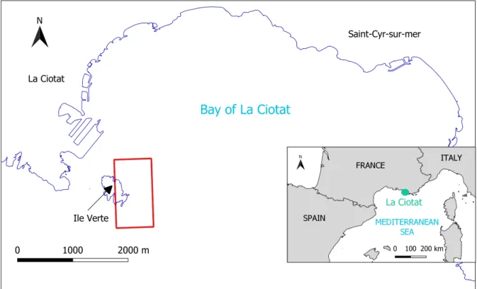
The chosen study site is called “Les Pierres”. It is located in the bay of La Ciotat (Provence-Alpes-Cˆote d’Azur, France), on the east of the island “Ile Verte”, see Fig. 2. Well-known by the scuba divers, the 0.8 km2 zone includes nine sub-zones (falls and reefs) which each presents an important marine fauna and various marine habitats (e.g. seagrass meadow, rocks with algal covers, coralligenous communities) between 10 and 60 m depth. The data sets were collected during spring and summer 2016 with the acquisition system described in the next subsection. During the surveys, bathymetric data, backscatter imagery and WCI were recorded.

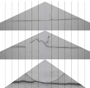
Fig. 1. Examples of WCI with different targets. Seabed is represented as a dark horizontal line. Top: sailing yacht (wreck, mast and spreaders); middle: bubbles from diver(s); bottom: school of fishes.

B. Acquisition system

As already mentioned, the MBES used for this acquisition campaign is a R2SonicT M _{2022. The R2Sonic swath is}

composed of 256 beams distributed over a maximal opening angle of 180◦, but usually over a 140◦ opening angle in a more common usage. The acoustic signal, emitted with a chosen frequency of 450kHz during a very short pulse length (15µs), was adapted to map with a high resolution (0.9°×0.9◦ angular opening) in shallow water (less than 100 m) [15]. The MBES was coupled with an inertial navigation system (INS) AplanixT M I2NS and a full Real Time Kinematic (RTK) Global Navigation Satellite System (GNSS). The whole devices provided a positioning precision of 1.0 cm on XY axes and 1.5 cm vertically, a rolling and pitching precision of 0.015◦ and a precision for heading trajectories of 0.02◦.

Two GPS antennas AeroAntenna Inc. AT1675-540 were used for satellite signal reception and navigation heading. Each offset of the whole system (sounder and positioning devices) was carefully measured at the vessels conception phase and regularly checked to avoid constant accuracy errors.

The navigation during acquisition was operated by a Ray-marine ACU 200 autopilot synchronised with the RTK GNSS using ViewMap, a Geographic Information System (GIS) and navigation software developed by C. Viala [14] which allows to trace and follow precise trajectories during acoustic data acquisition. The whole navigation system has an accuracy of 0.5 m to follow trajectories. Underwater sound velocity was constantly checked using a Valeport Ltd miniSVS sound velocity sensor mounted on the MBES. Additional underwater sound velocity profiles were performed with another miniSVS

Fig. 2. Location of the “Les Pierres” study site (red frame) on the French Mediterranean coast in the La Ciotat bay, near the “Ile Verte” island.

Fig. 3. Bathymetric 3D survey of the south-west part of the “Ile Verte” at La Ciotat bay (France), represented with a colour gradient. Red areas have a depth lower than 15m, yellow ones are between 15m and 30m depth, seabeds in blue are at least 45m depth. The zone corresponds to a 500m × 500m area.

to detect the possible presence of a thermocline or fresh water layers impacting on the sound propagation.

The whole acquisition system was finally composed of the R2Sonic 2022 MBES, the Aplanix I2NS INS, the two GPS antennas, the two sound velocity sensors and computers for the navigation, configuration of the MBES and acquisition-storage data. All these devices were boarded on the Seaviews One, a small vessel (6 m long) specifically designed for hydrographic surveys with a central shaft for the sounder, the navigation unit and the sound velocity probe. This light craft allows to follow the shore as close as needed with its low draught.

C. Mapping the seabed morphology and nature

After each survey, the data collected by this set of ac-quisition systems are first checked then merged before being mapped.

GNSS positioning data were post-treated with the open source program package RTKLIB. By taking into account the accuracy of each sensor, i.e. the RTK GNSS, the inertial navigation system, the MBES, the sound velocity sensor and the sound velocity profiles leading to horizontal and vertical errors, we obtained a XY accuracy of ± 0.078 m, and a Z total accuracy calculated according to

Zaccuracy= 0.009 + 0.0066 × D (1)

where Zaccuracy (in m) is the vertical error and D (in m) is the

depth.

Using the ViewSMF software [14], outliers and seabed miss-tracking points were also removed from the bathymetric data with the help of some filters.

Backscatter data were corrected in angle of incidence by using the sound velocity constant measurements and profiles. A time variable gain (TVG) was also run to avert noise from ping overload. Snippets (i.e. time series of data samples per beam) were computed too, in order to reduce the noise generated by the beam spreading on the bottom and thus, to increase the overall resolution of backscatter images.

Once all these pre-processing performed, the bathymetric maps have been realised. A 3D rendering of the south part of the “Les Pierres” site is presented in Fig. 3. The acoustic

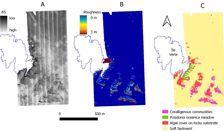
Fig. 4. Data from the acquisition survey mapped. A: the acoustic backscatter map, “sonar image”, the strength values are a no-dimension intensity. B: the computed roughness, with metric values. C: classification of the seabed nature.

backscatters are also mapped (Fig. 4A) and the roughness of the seabed is evaluated with the bathymetric soundings (Fig. 4B). According to this three maps (bathymetry, sonar and roughness), an automated classification of the seabed is established [16]. Ground thruth data were collected by scuba diving on the each rocky reefs as well on seagrass meadows that had not a high acoustic signature on the rocky substrate. The results are provided on the Fig. 4C.

III. DATA PROCESSING A. Introduction

As already said in the introduction, in the medium to long term, there are several reasons justifying a further exploitation of WCI. First, to endow the software that with develop, with new competitive tools for the detection and study of the fish activities from hydrographic MBES data. Secondly, to be able to realise environmental studies in addition to hydrographic surveys. And finally, to extend the tools devoted to the detection and the analysis of fish activities to any kind of WCI targets.

In order to demonstrate the feasibility and the interest of the aforementioned points, the software suite composed of ViewSMF and ViewMap was endowed with interfaces and extensions to handle this data set in 2017 [17], yet, the initial treatments were performed purely manually. At that time, with our software, it was possible to display the map of fish accu-mulation zones and then to perform fish classification before

correlating this information with the seabed. However, this manual method and more precisely the fish classification stage was time-consuming and had to be automated. To produce these maps - either with the manual or semi-automated method -, several successive stages are required:

• The reduction of the WCI to the part of interest (see

subsection III-B),

• The detection of pings exhibiting any activity (III-C), • The mapping of the fish accumulation zones (III-D), • The manual (III-E) or semi-automated (III-F)

classifica-tion of fishes and the mapping of the results.

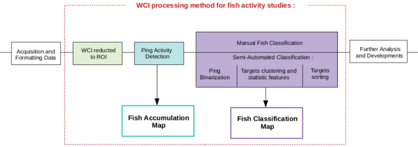
The Fig. 5 is a graphical depiction of the whole processing chain applied to WCI when fish activity studies are considered. B. Choice of the useful part of the WCI

The manual approach is not performed on the whole water column images: only their upper part is kept. It corresponds to the portion of the WCI which is not altered by the signal returned from the seafloor in interaction with the beam pattern-specific side-lobes. The limit between these two parts is fixed by the Minimum Slant Range (MSR) which stands for the shortest radial distance between the sonar transducer and the seafloor1. It is easier to detect and analyse targets above the

1_{For the record, the depth is a measure of the vertical distance below a}

system reference water level, whereas the range is a measure of the distance of the seabed to the MBES by taking into account the incidence angle.

Fig. 5. Block diagram of the global data processing chain applied to MBES. The first block “Acquisition and formatting data” refers to the section II. The block depicted by a dotted red line represents the successive stages needed to exploit the WCI, whereas the blocks behind arrows are the two produced maps. *ROI: region of interest.

minimum slant range also known as the “validity arc”, due to a better Signal-to-Noise Ratio (SNR).

For the calculation of the minimum slant range, two variants have been implemented in the ViewSMF software:

• The Standard Minimum Slant Range (SMSR) in (2) is

determined for every swath by the range of the minimum depth range point:

SMSR(p) = argmin

b∈[1,Nbm]

Dp,r(b) (2)

where SMSR(p) (in m) stands for the SMSR of the p-th ping, Dp,r(b) (in m) are the bathymetric points in range

distance r (in m) for the b-th beam of the p-th ping and Nbm is the beam number,

• The Gliding Minimum Slant Range (GMSR) in (3) is determined for every swath by the minimum of the SMSR along the previous-next i neighbour pings:

GMSR(p) = argmin

i∈[±10]

SMSR(p − i) (3) where GMSR(p) (in m) stands for the GMSR of the p-th ping.

It turns out that these two MSR are meaningful. Most of the time, the SMSR is sufficient and well determined. But, because of the side-lobes effect, a persistence phenomenon due to the bottom shape can appear in the WCI. Generally, it does not provoke any bottom miss-tracking, but some bottom persistent interferences overflow in the validity arc which can lead to a miss-interpretation of targets. That is why the GMSR, by taking into account the previous-next pings, is more robust than the MSR with regards to this possible persistence problem. An example of these two variants of the MSR in the case of a persistent bottom is provided on the Fig. 6. C. Ping activity detection

In order to evaluate the biological activity in a WCI, two indexes have been introduced: the average biomass (denoted

Fig. 6. An example of water column ping including fishes (indicated by the two grey circles) and some bottom persistent interference. The bathymetric points are marked by green points. The two different minimum slant ranges (symbolised by a yellow arc) are drawn (calculation based on the SMSR (top) or the GMSR (bottom)). The WCI had been thresholded at -70 dB above the MSR. Detected targets appear in white (fishes and a part of the interference).

by BAv) and the maximal biomass (denoted by BM ax). Here,

the “biomass” term, in an acoustic meaning, refers to the whole objects and living organisms that sign in a WCI, not the weight of the living organisms. The average biomass given in (4) estimates the average value of all the impulse intensity responses (in dB) within the validity arc:

BAv(p) = 1 Nbm× Nsp Nbm X i=1 Nsp X j=1 BSi,j(p), (4)

where BAv(p) (in dB) is the average biomass for the p-th

samples number in a beam before the MSR, BSi,j(p) is the

validity arc in backscatter strength value.

The value BAv should give an account of all the suspended

objects (e.g. fish, zoo-plankton) while the maximal biomass gives only an account of the strongest target signatures in the same zone. The maximal biomass is estimated by storing the n strongest intensity (in dB) samples among all the samples within the validity arc (the hyper parameter n is typically fixed at 100 in (5)). From the max-biomass, it is possible to compute the maximum, the minimum and the average among these n values: BM ax(p) = argmax BS0_{⊂BS,card(BS}0_)=n X bs∈BS0 |bs| (5)

where BM ax(p) (in dB) is the maximal biomass for the p

-th ping. The set BS is -the backscatter streng-th values of -the validity arc, i.e. BS = {BSi,j(p), ∀i ∈ {1, . . . , Nbm}, ∀j ∈

{1, . . . , Nsp}}. The subset of the n higher backscatter strength

values of BS is denoted by BS0. Its n elements are stored in a vector denoted by bs.

The biomass values from the ping in Fig. 6 are reported in the Table I.

TABLE I

COMPARISON OF THEBAvANDBM axVALUES VERSUS THEMSR

VARIANT. VALUES OBTAINED ON THEWCIGIVEN INFIG. 6 Biomass index MSR: Minimum Slant Range

Standard MSR Gliding MSR BAv(dB) -84.3 -87.9

BM ax- min (dB) -60.4 -66.9

BM ax- avg (dB) -58.3 -61.7

BM ax- max (dB) -53.2 -55.4

The difference between the MSR led to some differences in the biomass values. Especially in the BAv because the large

persistence near the bottom had higher backscatter intensities than the background noises, that skewed therefore the average, in the SMSR, which should be closer to the background noise value. The BM ax index was less affected by the bottom

per-sistence because its value was computed from the n strongest samples that can come either from the fishes or the persistence. Hence, since at least one target in a WCI is enough to make BM ax really higher than BAv, it is quite easy to distinguish

between pings exhibiting at least one target and those which do not. When there is no target in the WCI, the minimum of BM ax is much more close to BAv. So, it is easy to fix a

threshold value: 15 dB above BAvseems a good choice. Here,

in Fig.6, the threshold has been set at -70 dB, highlighting the targets that are present and sign with a higher value computed as the average value of BM ax.

D. Fish accumulation mapping

Once the biomass indexes are computed for each ping of the survey, this information can be charted. Each ping is represented by an intensity colour point on a map and positioned according to the vessel path. Since most paths do not exhibit fish activities, they are not drawn to better

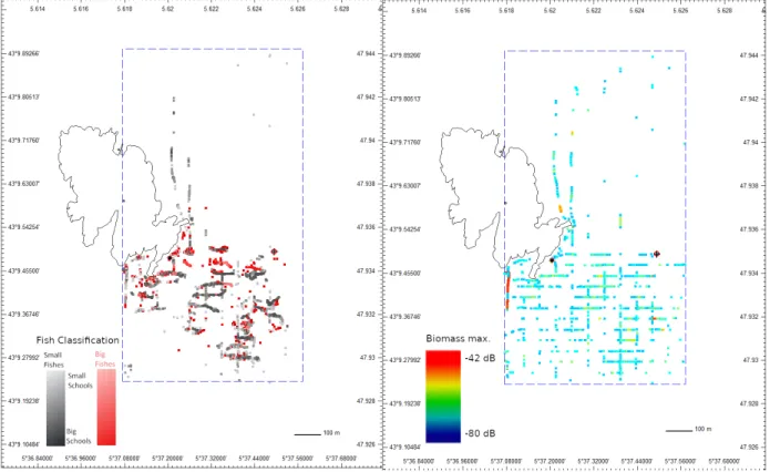
emphasise the pings with fish echoes and thus to better delimit the different fish accumulation areas. The fish accumulation map of the summer 2016 survey is given on the left side of Fig. 7. It tends to show that fishes are visibly concentrated on the south of the site “Les Pierres” where reefs are located. E. Manual fish classification

Since WCI provided sufficient details about individuals and fish schools, a classification was attempted. Actually, from on ping to one other, fishes swum at different depths, had various sizes and evolved within more or less large schools. The manual classification was established according to these three parameters. The software ViewSMF, dedicated to the MBES data processing, was endowed with an interface to quickly browse the pings including any detected fish and then to assign the targets to a class. Targets were spotted in the frame by circling them (as in the Fig. 6). Four sizes of circle were available for classifying the size of the schools but also two colours for classifying the fishes in little or big categories. The position of the circle in the frame automatically classified the targets according to their depth - surface, column and near seabed. An example of a result of the manual classification is visible on the right of Fig. 7.

This first manual method for the mapping of fish accumu-lation areas and fish classification proved that studying fish activities in very shallow water with a hydrographic MBES is utterly practicable. However, this manual classification was really fastidious and time-consuming and had to be automated prior to any other improvement of the rest of the method. This is described in the next paragraphs.

F. Semi-automated fish classification

The automation of any method generally requires more pre-processing to be really efficient. Thus, a semi or completely automated classification still could not be done from the data at the end of the ping activity detection step III-C. In fact, this stage had to take a binary decision about the WCI content -empty or not -empty (i.e. containing fish target or whatever)) - but was not yet designed to detect all the targets. In this subsection, the first step is to binarize properly the WCI with any target, then to cluster the different target(s) before computing for each of them, the statistical features that were used to sort the fishes as previously described. At the end of this semi-automated classification, the results should be roughly equivalent (or better since less subject to assessment errors).

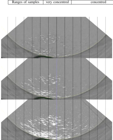
1) Ping binarization: After considering the whole data set, we chose to manually threshold the WCI. In average, the values of the background noise ranged between 90 dB and -100 dB. The strongest backscatter objects have samples which start to be detected at -65 dB, whereas from -80 dB, nearly all the samples of a target are effectively detected. A too high value threshold (like -70 dB) does not seem to be adapted since the targets are still incomplete. On the contrary, a too low value threshold (like -90 dB) might not be adapted either since it may happen that close targets are merged in one single

Fig. 7. Left: fish accumulation areas on the site “Les Pierres” represented by the value of the maximal biomass of every ping (summer 2016 survey). Right: fish classification on the site “Les Pierres” categorising fishes detected during the summer 2016 survey in four classes (big or small individuals in large or small fish schools).

target. Finally, a fixed threshold with a value between the aforementioned cited values is often a good compromise, even if some false alarms may appear and considered as targets like the fishes. An example of different values for the threshold is provided in Fig. 8.

Thus, at that time, a range of several threshold values adapted to the current survey was evaluated by hand during the data discovery and then fixed as an “hyperparameter” for the rest of the method.

2) Targets clustering and statistical features: Once the WCI thresholded, it is possible to agglomerate the samples into cluster corresponding to the detected targets (even the false alarms). The method simply browses the WCI values until it finds a sample above the threshold value and then search the neighbouring samples which belong to the same cluster (and also the target). For further treatments, only the coordinates - depth range and angle, corresponding respectively to row and column of a classical image - of the clustered samples are stored. From these clusters and their coordinates, some statistical features are computed. The aim of these features is then to sort the targets into two classes: i) detection of interest (like fishes), ii) detection that do not interest us in this application (e.g. wake, noise, scuba diver bubbles) and false alarms. The chosen statistical features are divided into three components: the depth range, the angle of the beam and the backscatter intensity. For each components of every targets, the minimum and maximum value are stored but also the mean

and the standard deviation. Thanks to these statistical features, it is then possible to compute the centroid and the size of every targets and then to establish sorting rules.

3) Sorting the targets: Since it is a semi-automated classi-fication, the rules to sort the targets were fixed heuristically. The knowledge of the survey data can allow to express the distinction between targets that interests us - fishes - and those which do not. As an example, fishes can be recognised by their small amount of samples and a round shape (angle and range sprawls are close) when false alarms correspond to very few samples and noise do not exhibit a constant form (persistence: very large patches, arc side lobes: an angle sprawl bigger than this in range). The table II of sorting rules for different targets is given below as examples. Afterwards, the fishes can be classified according to different parameters: i) their position in the water column thanks to the computed centroid (range position), ii) their size thanks to the quantity of samples and finally according to iii) the size of the schools taking into account the number of fishes detected in the WCI.

IV. DISCUSSION

Our main goal was to give an estimation of the fish activity -accumulation areas and classification - during a survey realised with a hydrographic MBES. A manual method was developed in 2017 and implemented in our software through GUIs. It allowed to obtain, as results, the maps of fish accumulation

TABLE II

VARIOUSWCITARGETS DISCRIMINATED ACCORDING TO THEIR COORDINATES AND INTENSITY.

Features WCI Targets

False alarm Arc side-lobes Fish Vessel Wake Bottom persistence Number of samples very few - fixed range of few a large number a large number Centroid of samples - - - near the surface near the bottom Backscatter intensity very low low in the edges, higher in center - -

-Angles of samples very concentred very sprawling concentred - -Ranges of samples very concentred concentred concentred -

-Fig. 8. WCI exhibiting fish school for different values of the chosen threshold: 70 dB (top), 80 dB (middle), 85 dB (bottom).

and classification and thereby to assert the feasibility of the proposed approach.

On the WCI collected by a well-resolved MBES in very shallow water, it is currently possible to visually distinguish the fish echoes from other targets echoes (e.g. bubbles, moor-ing line, wake, bottom persistence, etc.) [18]. Moreover, the fish schools can be distinguished from the individuals and then, the individuals can be classified according to their size. This evaluation remains therefore essentially qualitative since fish size can not be precisely estimated due to i) the WCI resolution and ii) the fact that the fish signatures do not necessarily reflect the whole fish since it is essentially the swim bladders that sign.

The suggested approach developed in this work provides the fish biomass map (in an acoustical meaning) of the studied areas and enables to identify the sub-areas where fishes are concentrated. Although this type of maps cannot achieve the estimation of the quantity of all the present fishes

-i.e. only fishes in the water column, rocky reef fishes can not be detected - it remains sufficient to locate the main fish pelagic living zones. The cross-analysis of bathymetry, marine habitats and fish biomass maps have led to retrieve some hardly surprising facts. Over the last decades, numerous studies have highlighted that fish accumulations are more likely located on sites with complex seascapes (such as rocky reefs and seagrass meadows) than on flat deeper zones [19] [20]. Likewise, the surveys, realised at different seasons in a year, allow to correlate the water temperature with the size of the fishes and their schools [21] [22]. In summer, with a thick thermocline, there were larger schools with big fishes than in winter, where little fishes seem to swim in small schools. This remark allowed to assert the second purpose of this study which was to correlate the fish activities with their environment (seabed morphology and nature).

Our results also suggest that it is possible to compare the areas with each other. For examples, the fish abundance within or at the edge of a protected marine area can be mapped. This type of study had been realised in 1995 not far from our study site (Carry-le-Rouet, France) by monitoring two types of species [23]. In this case, acoustical measures could complete visual evaluations. Likewise, it is possible to compare the areas over time. For examples, it would consist of realising a seasonal monitoring to attest that fishes have settled on artificial reefs [24] or to compare their attractiveness against the one of natural reefs [25].

At that point, the analysis process described previously does not allow any precise abundance evaluation or species identifi-cation of fish schools without additional information. It offers benefits nevertheless. As an additional data of hydrographic surveys, it remains a way to quickly acquire fishery data for the first time in a wide area. Once the fish accumulation have been drawn, it can lead to more specific surveys where traditional fish counting methods can be used. In this way, measuring fish accumulation do not replace specific fishery monitoring techniques, but provides additional spatial data through the analysis of biological indexes. For instance, if fish assemblage tracking and counting is now possible with cameras which can be fixed and active for a long time, they are efficient only if they were set up in the interesting places [26] that our method can highlight.

Gaining in precision for abundance evaluation and species identification of fishes is conceivable in the future. It will not be possible without additional information however. For the

first task, it requires a calibration of the MBES with targets of known size. This is made possible with underwater cameras or by scuba divers. For the second task, it requires the knowledge of locals divers, fishermen, environmental administrators who are familiar with the main local marine species and their habits.

This study has a great potential for current and coming applications as described above, but also a technical po-tential since the method still remains mostly manual. More Specifically, the manual classification was fastidious and time-consuming. For this reasons, more autonomous techniques were required and thus a semi-automatic classification was presented. This new contribution brought two major advan-tages: (i) when the manual classification could take day(s) to be properly done, the new one takes a few minutes at worst; (ii) this allowed to deepen the exploitation of the WCI and prepare the data to be used with more autonomous techniques (like machine learning).

Before going further in the WCI exploitation, other steps of the process need a deeper study. Among others, the number of pings considered for the gliding-MSR and the number of strongest samples kept to compute the BM ax value were this

time fixed by hand. For the gliding-MSR, the number of ping had to be adapted to the situation since the bottom persistence can liner more or less longer according to the intensity of the original bottom. About the number of samples kept to the maximal biomass (n=100), n was fixed with an absolute value, but it should be adapted to the size of the WCI above the minimum slant range which can vary from one ping to another. Finally, the thresholding pre-processing before the clustering should be automatically computed prior to the gliding-SMR or the maximal biomass modification. Actually, with a well-chosen threshold, the ping activity detection and the ping binarization could be done in one stage for a WCI being always truncating with the standard-MSR.

The main difficulties to properly automatically threshold the WCI, from survey to survey and from ping to ping, are raised by the background noises due to the inhomogeneous and randomly distributed sea clutter2. Since the noises do not follow a Gaussian distribution and vary with the depth, classical methods such as the Otsu binarisation (adaptive image thresholding method) or global thresholding techniques were not really suitable. Thus, local thresholding techniques may be considered such like adaptive methods with a median kernel, or the use of a wavelet method as proposed in [28], and else combining image and learning methods like in [29].

CONCLUSION

The innovative WCI technique of analysis developed in this work, and its future improvements, have the potential to provide in a near future exhaustive surveys of the seafloor, as

2_{The sea clutter is a term used for unwanted echoes in electronic systems,}

particularly in reference to radars. This term can be extended to sonars since the sea is a noisy environment due to the characteristics of underwater acoustic and to various noise origins (i.e. marine traffic, rain and surface waves, marine organisms, thermal noise) [27].

well as of the water column, thanks to a single sensor: the multibeam echosounder. Combining high resolution maps of marine habitats with fish assemblages are mandatory to fall in the scope of the global effort to investigate, monitor and evaluate the ecological status of fundamental coastal marine ecosystems. This is especially true in the framework of the European Marine Strategy Framework Directive (MSFD) that aims to apply an ecosystems-based approach in the regulation and management of the marine environment, marine natural resources and marine ecological services. In the Mediterranean Sea, the MSFD targets, among others, the fundamental ecosys-tems based on P osidonia oceanica meadows as well as those relying on coralligenous communities. As demonstrated in this study, compact MBES have the potential to provide a complete spatial evaluation of these habitats, even when they are mixed with other habitats such as rocky and sedimentary substrates. Overall, such an approach allows to decrease the cost of environmental underwater studies by increasing their efficiency in connection with the size of the area exhaustively investigated.

ACKNOWLEDGMENT

This work has been made possible thanks to the Agence de l’Eau RMC which financed the hydrographic surveys in 2016 at La Ciotat and the first research works on the underwater biological activity. Special thanks as well to the Association Nationale de la Recherche et de la Technologie (ANRT) for the “Convention industrielle de formation par la recherche (CIFRE)” service allowing the funding of a tripartite PhD thesis between a PhD student, a society and a research laboratory.

REFERENCES

[1] Abadie A., Viala C., “Le sondeur multifaisceaux en hydrographie : utilisations actuelles et futures”. XYZ 157, pp. 17-27, Dec. 2018 [2] Hassan R.C., Ierodiaconou D., Laurenson L., Schimel A., “Integrating

Multibeam Backscatter Angular Response, Mosaic and Bathymetry Data for Benthic Habitat Mapping”. PLOS ONE, Volume 9, Issue 5, May 2014.

[3] Colbo K., Ross T., Brown C., Weber T., “A review of oceanographic applications of water column data from multibeam echosounders”. Estuarine, Coastal and Shelf Science, vol. 145, pp 41-56, 2014 [4] Løvik A., Hovern J.M., “An experimental investigation of swimbladder

resonance in fishes”. The Journal of Acoustical Society of America, 66, pp 850-854, 1979.

[5] Chu D., “Technology evolution and advances in fisheries acoustics”. Journal of Marine Science and Technology, 19, pp 245-252, 2011. [6] Innangi S., Bonanno A., Tonielli R., Gerlotto F., Innangi M., Mazzola

S., “High resolution 3D shapes of fish schools: a new method to use the water column backscatter from hydrographic Multi-beam Echo Sounders”. Applied Acoustics, 111, pp 148-160, 2016

[7] Holmin A.J., Handegard N.O. Korneliussen R.J., Tjosthein G., “Simula-tion of multi-beam sonar echos from schooling individual fish in a quiet environment”. The journal of Acoustical Society of America, Vol 132, Issue 6, 2012.

[8] Nøttestad L., Fern¨o A., Mackinson S., Pitcher T., Misund O.A., “How whales influence herring school dynamics in a cold-front area of the Norwegian Sea”. ICES Journal of Marine Science, 59, pp 393-400, 2002 [9] Cutter G., Demer D.A., “Accounting for scattering directivity and fish behaviour in multibeam-echosounder surveys”. ICES Journal of Marine Science, Vol. 64, pp 1664-1674, 2007.

[10] Misund O.A., Aglen A., “Swimming behaviour of fish schools in the North Sea during acoustic surveying and pelagic trawl sampling”. ICES Journal of Marine Science, Vol. 49, Issue 3, pp 325-334, 1992.

[11] Gurshin C.W., Jech J.M., Howell W.H., Weber T.C., Mayer L.A., “Measurements of acoustic backscatter and density of captive Atlantic cod with synchronized 300-kHz multibeam and 120-kHz split-beam echosounders”. ICES Journal of Marine Sciences, Vol. 66, pp 1303-1309, 2009.

[12] Trenkel V.M., Mazauric V., Berger L., “The new fisheries multibeam echosounder ME70: description and expected contribution to fisheries research”. ICES Journal of Marine Sciences, Vol. 65, Issue 4, pp 645-655, may 2008.

[13] Mosca F., Matte G., Lerda O., Naud F., Charlot D., Rioblanc M., Corbi`eres C., “Scientific potential of a new 3D multibeam echosounder in fisheries and ecosystem research”. Fisheries Research, 2015. [14] Viala C., ViewMap and ViewSMF softwares. 2015. https://seaviews.fr/

en/services-3/software-development [Accessed 18th April 2019] [15] Sonic 2024/2022 Broadband Multibeam Echosounders, Operation

Man-ual V5.0, 2014.

[16] Abadie A., Marty P., Viala C., “BATCLAS index: a new method to identify and map with high resolution natural and artificial underwater structures on marine wind turbine sites. 3rd Wind Energy and Wildlife seminar”. Artigues-pr`es-Bordeaux, France, pp 120-127, 2017. [17] Viala C., Abadie A., “Mesure de l’activit´e biologique par sondeur

multifaisceau”. Study report from Seaviews to Agence de leau RM& C. 51 pages, 2017.

[18] Schneider von Deimling J., Weinrebe W., “Beyond Bathymetry: Water Column Imaging with Multibeam Echo Sounder Systems”. Hydro-graphische Nachrichten, Vol. 31, pp 6-10, feb 2014.

[19] Cal`o A., F´elix-Hackradt F.C., Garcia J., Hackradt C.W., Rocklin D., Trevi˜no Ot´on J., Charton J.A.G., “A review of methods to assess connectivity and dispersal between fish populations in the Mediterranean Sea”. Advances in Oceanography and Limnology, Vol. 4, Issue 2, pp 150175, 2013.

[20] Charbonnel E., Serre C., Ruitton S., Harmelin J.-G., Jensen A., “Effects of increased habitat complexity on fish assemblages associated with large artificial reef units (French Mediterranean coast)”. ICES Journal of Maritime Sciences, Vol. 59, pp 208213, 2002.

[21] Palomera I., Olivar M.P., Salat J., Sabat´es A., Coll M., Garc´ıa A., Morales-Nin B., “Small pelagic fish in the NW Mediterranean Sea: an ecological review”. Prog. Oceanogr, Vol. 74, Issue 2-3, pp 377396, 2007. [22] Sabat´es A., Mart´ın P., Lloret J., Raya V., “Sea warming and fish distribution: the case of the small pelagic fish, Sardinella aurita, in the western Mediterranean”. Global Change Biology, Vol. 12, Issue 11, pp 22092219, 2006.

[23] Harmelin J.G., Bachet F., Garcia F., “Mediterranean Marine Reserves: Fish Indices as Tests of Protection Efficiency”. Marine Ecology, Vol. 16, Issue 3, pp 233-250, Sept. 1995.

[24] Clark S., Edwards A.J., “Use of Artificial Reef Structures to Rehabilitate Reef Flats Degraged by Coral Mining in the Maldives”. Bulletin of Marine Sciences, Vol. 55, numbers 2-3, pp 724-744, Sept. 1994. [25] Carr M.H., Hixon M.A., “Artificial Reefs: The Importance of

Compar-isons with Natural Reefs”. Fisheries Magazine, Vol. 22, Issue 4, pp 28-33, April 1997.

[26] Boom J.B. et al, “Long-term underwater camera surveillance for mon-itoring and analysis of fish populations”. International Conference on Visual observation and Analysis of Animal and Insect Behaviour, 4 pages, Jan. 2012.

[27] Lurton X., “Acoustique sous marine : presentation et applications”. Edition Quae, Plouzan´e, France, 1998.

[28] Karthikeyan K., Chandrasekar C., “Speckle Noise Reduction of Medical Ultrasound Images using Bayesshrink Wavelet Threshold”. International Journal of Computer Application, Vol. 22, Issue 9, pp 8-14, may 2011. [29] Hofmann, M., Tiefenbacher P., Rigoll G., “Background segmentation with feedback: the pixel-based adaptative segmenter”. IEEE Computer society Conference on Computer vision and pattern recognition work-shops, 2012.