HAL Id: hal-01893141
https://hal-amu.archives-ouvertes.fr/hal-01893141
Submitted on 11 Oct 2018
HAL is a multi-disciplinary open access
archive for the deposit and dissemination of
sci-entific research documents, whether they are
pub-lished or not. The documents may come from
teaching and research institutions in France or
abroad, or from public or private research centers.
L’archive ouverte pluridisciplinaire HAL, est
destinée au dépôt et à la diffusion de documents
scientifiques de niveau recherche, publiés ou non,
émanant des établissements d’enseignement et de
recherche français ou étrangers, des laboratoires
publics ou privés.
To cite this version:
Y. Trardi, Bouchra Ananou, Z. Haddi, M. Ouladsine. Multi-Dynamics Analysis of QRS Complex
for Atrial Fibrillation Diagnosis. 2018 5th International Conference on Control, Decision and
In-formation Technologies (CoDIT), Apr 2018, Thessaloniki, France. �10.1109/CoDIT.2018.8394935�.
�hal-01893141�
Abstract—This paper presents an effective atrial fibrillation (AF) diagnosis algorithm based on multi-dynamics analysis of QRS complex. The idea behind this approach is to produce a variety of heartbeat time series features employing several linear and nonlinear functions via different dynamics of the QRS complex signal. These extracted features from these dynamics will be connected through machine learning based algorithms such as Support Vector Machine (SVM) and Multiple Kernel Learning (MKL), to detect AF episode occurrences. The reported performances of these methods were evaluated on the Long-Term AF Database which includes 84 of 24-hour ECG recording. Thereafter, each record was divided into consecutive intervals of one-minute segments to feed the classifier models. The obtained sensitivity, specificity and positive classification using SVM were 96.54%, 99.69%, and 99.62%, respectively, and for MKL they reached 95.47%, 99.89%, and 99.87%, respectively. Therefore, these medical-oriented detectors can be clinically valuable to healthcare professional for screening AF pathology.
I. INTRODUCTION
AF or A-fib is the most common type of cardiac arrhythmia, which has a severe impact on life quality and increases the risk of stroke, and heart failure [1]. Rapid and efficient method of diagnosis is required to create a flexible machine that can detect the AF occurrence in ECG signal. Further, different algorithms have been proposed in the literature for automatic AF detection and classification. Most reported studies are based only on inter-beat time series. These inter-inter-beats are usually called RR segments by the cardiologist community, which can be computed by measuring the time difference between two successive R-peaks (detected in the QRS complex). The RR segments can be considered as a dynamic that describes the rhythmic behavior of the heartbeat signal. Indeed, we have addressed four dynamics of the QRS complex. This new methodology was first proposed by [2], which was focused on the analysis of different characterizations within the time series interval of the heartbeat signal. Further, we could assume that each dynamic is considered as a sensor that produces more knowledge about database characteristics. Several methods have been proposed in the literature for automatic cardiac arrhythmia detection and classification, such as Neural Network [3], Fuzzy C-Means clustering [4], Wavelet Transform and Support Vector Machine [5], Autoregressive Modeling [6], Bayesian methods [7], and many others. These reported studies focused on variables extracted from RR interval time series or the analysis of the ECG
Y. Trardi, B. Ananou, Z. Haddi and M. Ouladsine are with Aix-Marseille Univ, Université de Toulon, CNRS, LIS UMR 7020, Marseille, France. (phone : 0033-753-992782 ; e-mail : [email protected]).
signal. However, the current study proposes a multivariate analysis that aimed to couple fourteen linear and nonlinear functions with the four aforementioned dynamics. Finally, for an effective AF detection, we applied support vector machine (SVM) and multiple kernel learning (MKL) classification algorithms using a combination of 56-feature.
II. MATERIAL AND METHODS
A. Database treatment
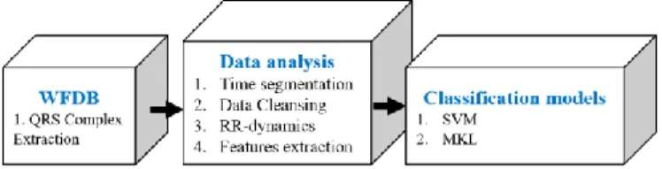
The proposed methods in this paper was evaluated on PhysioBank free accessible databases, called Long-Term AF Database including 16078 AF and 18502 NSR episodes. The operation procedures performed in this study were separated into three parts as shown in (Fig. 1). The first part is ECG signal processing to extract the QRS complex; the second part is dedicated for data analysis; and finally, the last part is for the training of classification models.
Figure 1. The data reprocessing and classification blocks
1) The QRS complex extraction
Figure 2. Thresholding peaks in signal
Firstly, WFDB (WaveForm DataBase) Software Package-Physionet is used to extract the QRS complex from each ECG recording. WFDB is a set of MATLAB functions and wrappers
Multi-Dynamics Analysis of QRS Complex for Atrial Fibrillation
Diagnosis
for reading, writing, and processing files in the PhysioBank databases formats. The WFDB process is used to generate two vectors: the first one concerns R-peaks location in the QRS complex (Fig. 2) and the second shows the annotations of each interval.
2) Data analysis
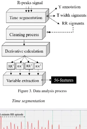
We have developed a data reprocessing algorithm containing four operational blocks described by: time segmentation; cleaning process; RR dynamics calculation; and features extraction; as shown in (Fig. 3). This process takes the R-peaks interval as input and provides the following outputs: RR segments; a repertory called T contains the width of each segment extracted from the R-peaks signal; a repertory called Y contains the annotations affected to each segment. Generally, Y could have several arrhythmias that are exchanged. In our study, we targeted NSR and AF rhythms.
Figure 3. Data analysis process
a) Time segmentation
Figure 4. Illustration of 1-minute segmentation process
The R-peaks signal extracted by the WFDB process must be segmented, we have chosen a 1-minute window to divide it into a set of RR segment as defined by equation (1).
RRR(2N) R(1 N 1) (1) Where N is the total number of components in the R-peaks signal. Another important parameter that must be chosen is the slip pitch. Generally, the slip pitch must be lower or equal to the splitting window. In the current study, we choose a slip pitch equal to 1-minute, as showed in Fig. 4.
b) Cleaning process
Each 1-minute segment RR is subjected to some constraints that must be respected. Firstly, the components of the 1-minute segment RR are bounded. All RR(n) values must be included in [0.3s, 2s], which means that, between two successive R-peaks, we cannot have a duration greater than 2 seconds or less than 0.3 second. Secondly, the duration of 1-minute segment RR should not exceed T(60 ) seconds. In this study, we have fixed equal to 2 seconds. This constraint is of great importance when a timeout is encountered during the ECG recording (or messing peak’s detection).
c) RR-dynamics
The dynamics employed in this investigation are described as follow:
- The first dynamic is redescribed as: 1 RR R(2N)R(1N 1), (2) - Second dynamic:
2 1 1 RR abs RR (2N)RR (1N 1) (3) - Third dynamic:
3 2 2 RR abs RR (2N)RR (1N 1) (4) - Fourth dynamic:
4 3 3 RR abs RR (2N)RR (1N 1) (5) d) Variable extractionVarious measures of complexity were developed to compare time series and distinguish regularity, chaotic and random behavior. Linear and nonlinear variables are used for the analysis of heartbeat time series signal.
The extracted features, used in this study, correspond to those listed in previous related works. All of them are applied to each of the four dynamics. For a better understanding, we use an index (i) to differentiate between dynamics, and we use the parameter N to represent the number of components in the ith dynamics.
(1) Linear analysis
RMSSD: is a time-domain method used to quantify the heart variability (HRV). This refers to the root mean square of successive RR components within each segment. The equation to describe RMSSD is giving: N i n 1 1 RMSSD RR (n) N
(6) MMedians: This refers to the median of medians, calculated by dividing the RR interval into three segments. Each segment was centralized by subtracting his own average value. Next, we calculate the median for each segment. And finally, a median of the three medians was calculated.SDSD: This refers to the standard deviation of differences between the adjacent RR components within each segment.
Kurtosis: is the ratio of the fourth moment and the second moment squared.
N i 4 n 1 2 N i 2 n 1 (RR (n) Mean) Kurtosis N (RR (n) Mean)
(7)Skewness: is the ratio of the third moment and standard deviation cubed.
N i 3 n 1 3 2 N i 2 n 1 (RR (n) Mean) Skewness N (RR (n) Mean)
(8) (2) Non-Linear analysisNine nonlinear methods were also investigated to characterize the studied arrhythmia. Four of them were based on the scatter plot of the RR segment [8].
VAI: Vector Angular Index is calculated as: N
n n 1
VAI
45 N (9) Where n is the angle between the line plotted from every scatter point to the original point and the x-axis, N is the number of scatter points.VLI: Vector length Index is calculated as:
N 2
i n 1
VLI
(lL) N (10) Where l is the length between every scatter point and the i original point, L is the mean of all the l , and N is the number of i scatter points.SD1: is the standard deviation calculated as:
i i
n 1 n
SD1var RR RR 2 (11) SD2: is the standard deviation calculated as:
i i i
n 1 n
SD2var RR RR 2 2 Mean(RR ) (12)
Where RRin RR (1i N 1), RRin 1 RR (2i N), and the
Var . is the standard deviation.
The five remaining variables were based on different types of entropy which provide a valuable tool for quantifying the regularity of physiological time series. For each type of entropy, a set of certain common parameters is needed to be initialized: embedding dimension m, tolerance threshold r and time series length N.
Following recommendations of some works dealing with these parameters [9], m was set at 2 and r represents 20 or 25% of the standard deviation RR segment. In the present study, we have used the following entropy methods.
ApEn: Approximate entropy was developed by Pincus [9,10] as a measure of regularity to quantify levels of complexity within time series.
SampEn: like ApEn, Sample entropy is a measure of complexity. But it is different from ApEn mainly by two points: (1) SampEn does not count self-matches; (2) SampEn does not use a template-wise approach [11,12].
FuzzyEn: Fuzzy entropy, a new measure of time series regularity. Like the two existing related measures ApEn and SampEn, FuzzyEn is the negative natural logarithm of the conditional probability excluding self-matches and considering only the first N-m vectors of length m. There are three parameters that must be fixed for each calculation of FuzzyEn: m, r and n defined as the gradient of the boundary of the exponential function [11].
COSEn: called coefficient of sample entropy, has a high degree of accuracy in distinguishing AF from NSR in 12-beat calculations performance [13].
QSE: Quadratic entropy rate, based on densities rather than probability estimates. To normalize the value of r, SampEn was modified by dividing the probability by the length of the overall tolerance window 2r [13]. All these 14-linear and nonlinear features were applied on each dynamic. As results, a set of 56 features was formed. In particular, three features were eliminated because they contain many of indeterminate value components given by the three methods SampEn, QSE, and COSEn. Once the data preprocess is done, the next obvious step is classification methods. SVM and MKL based algorithms were developed for the classification task. We should notice that we have created our own algorithms based on the same theory given in each method.
B. Classification methods
1) Support Vector Machine (SVM)
Currently, support vector machines (SVM) have proven to be an extremely effective tool for solving learning problems such as classification or regression [14]. The SVM, introduced by Vladimir Vapnik in the 1990s is a category of supervised algorithms designed to constructs a hyperplane or a set of
hyperplanes in a high- or infinite- dimensional space [15]. In the classification problems, we are given a training data set of couple-subject:
x , y ,1 1
, x , y
n n
, where x a vector i subject and yi 1 a target indicating to which class belongs each subject x . The traditional problem of SVM algorithm is to i establish a characteristic function able to identify correctly all the learning dataset:D x
yi. In general, the decision function is written as:
T
D x sign w xb , (13)
Where the equation w xT b is the characteristic function, with w p and b are the parameters that defined the optimal hyperplane. For a given C0 [16] and [17] have suggested the following optimization problem:
n T i i 1 w,b, T i i i i 1 min w w C 2 subject to : y (w x b 1 , 0, i
Where n is the total number of subjects,
xi is a nonlinear function that maps the training patterns into high-dimensional feature spaces. The parameter i is a slack variable and C is the penalty parameter of the error term, which must be adjusted in order to maintain the compromise between a better margin of separation and a better generalization of the decision. To solve (14) we adopt the Lagrangian formulation with constraints defined as follows:
n n i j i j i j i i, j 1 i 1 i n i i i 1 1 min y y K x , x 2 0 C subject to : ; i y 0
(15)Where the kernel function is K x , x
i j
T
xi
xj , which represents the scalar products in feature space, and i are Lagrange multipliers. Once the optimization is done, these Lagrange multipliers are produced and used to determine the parameters w and b that define the optimal separator hyperplane:
k s s s s 1 w y x
(16)
k n s r r r s s 1 r 1 1 b y y K x , x k
(17)Where each index (s) defines the active constraints at the optimum, where y (ws T
xs b)1. These indices (s) are obtained by extracting the positions of the Lagrangian multipliers that are strictly greater than zero (called support vectors indices). Then, the classification decision for a test
x which was not included in the training set is given by:
n
s s s s 1 y x sign y K x, x b
(18)2) Multiple Kernel Learning (MKL)
MKL was first proposed by Lanckriet et al, considered conic combinations of kernel matrices for binary classification, resulting to a convex quadratically constrained quadratic programming problem [18]. Most published studies on MKL are focused on two issues, (i) how to improve the classification accuracy of MKL, and (ii) how to improve the learning efficiency. Several approaches were proposed to learn an appropriate kernel combination, including ℓ1-norm [19], ℓp-norm [20], entropy-based [21], and mixed ℓp-norms [22]. The reasons to use MKL is their ability to learn from a larger predefined set of kernels and parameters an optimal linear (or nonlinear) combination of kernels. In order to identify a robust resolution of a machine learning problem. As well, instead of creating a new kernel, MKL algorithm can be used to combine kernels already established.
In this study, we have applied the MKL theory for the binary classification, that was developed by [23]. For any problem of kernel algorithms, the solution of the learning problem is always given by (18). Where the kernel K(.,.) is a convex combination of basis kernels given by:
M
M m m m m m 1 m 1 K x, x ' d K x, x ' , for d 0, d 1
(19)Where M is the total number of kernels. The problem of the data representation through the kernel is then transferred to the choice of weights d . m
The used MKL algorithm is a weighted ℓ2-norm regularization, or the ℓ1-norm constraint on the vector d is a sparsity constraint that will force some weights d to be zero. In m the MKL framework, the decision function f(x)
m mf (x) is a combination of different fm(x) functions each affected to a kernel K . Further, the solution of the primal MKL problem is m calculated by solving the following convex equations:m 2 m i f ,b, ,d m m i i m i i i m m m m 1 1 f C min 2 d y f (x ) b 1 0 subject to: d 1 d 0 m
(20)To solve (20) we consider the following constrained optimization problem:
m m
d m
Where: m 2 m i f ,b, ,d m m i i m i i i m 1 1 f C min 2 d J(d) y f (x ) b 1 0 i
(22)Then we give the Lagrangian formulation of (22) with the combined kernel as:
n M n i j i j m m i j i i, j 1 m 1 i 1 i n i i i 1 1 y y d K x , x max 2 0 C subject to : ; i y 0
(23)To solve (21) we use a simple gradient method. Then, to solve (23) we put all dm 1 M , and we follow the same structure process adopted in the SVM algorithm.
J(d) is considered as the optimal objective value of (23). Because of the strong duality, J(d) is also the objective value of the dual problem:
n M n i j i j m m i j i i, j 1 m 1 i 1 1 ˆ ˆ ˆ J(d) y y d K x , x 2
(24) Where ˆ maximizes (23). After J(d) has been calculated, we solve (21). We start by calculating the derivatives of J(d) as if ˆ does not depend on d.i j i j m i j i, j m J 1 ˆ ˆ y y K (x , x ), m d 2
(25)Then we compute the reduced gradient of J(d) as follow:
m red m m m J J for m d d J J J for m d d
(26)Where d is the greatest component of the vector d and its index. Next, the descent direction for updating d is given by:
m m m m m m m m m d 0 J J 0 if d 0 and 0 d d J J D if d 0 and m d d J J if d 0 and m d d
(27)Once the gradient of J(d) and the descent direction D were computed, we start the process of updating d by using:
max
d d D (28) Where max is the maximal admissible step size headed by D, and calculated by: max dv Dv (29) Where: m m m m/ D 0 v arg min d / D (30) If we replace the value of max in (28) we get
v v
d d ( d D ) D (31) The Eq. 31 in a matrix form is given by
v v 1 1 1 v v v v v v v M M M ( d D ) D d d ( d D ) D d d ( d D ) D d d (32)
We can notice that component v of the vector d becomes null. After the first update, now we compute J (d)* using an SVM solver with K
md*mK ,m where d* d maxD, and we check if the objective value decreases or not
*
J (d)J(d) . In the first iteration we set J (d)* J(d). If the objective value
decrease, d is updated using the formula d d maxD, which implies that dv0 and we set J(d)J (d).*
This procedure is repeated until *
J (d) stops decreasing. To end up this process, we calculate an optimal step size by applying the golden search method on the interval between 0 and
max,
with an appropriate stopping criterion, such as the Armijo rule. Then the last adjustment is executed to compute the optimal value of d as d d D.
Finally, the whole algorithm procedure is terminated when a stopping criterion is achieved. This stopping criterion can be either based on the duality gap, the KKT constraints, the variation of d between two consecutive steps, or, a maximal number of iterations. In this current study, we used MKL duality gap giving by:
n i j i j m i j m i, j 1 n * i j i j m m i j i, j 1 mDyalGap DualOne DualTwo ˆ ˆ DualOne max y y K x , x Where : ˆ ˆ DualTwo y y d K x , x
(33)Consequently, we stop the process when DualGap, where a tolerance threshold.
III. RESULTS
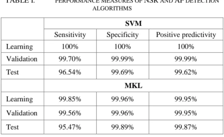
Tab.1 summarizes the performance obtained for SVM and MKL algorithms. In this study, two rhythms episodes of AF and NSR were extracted from Long-Term AF Database. SVM and MKL based-algorithms were optimized by using various configurations including the kernel function (Linear function, polynomial function, radial basis function), its corresponding adjustment coefficients, and the regularization parameter C. In order to get the optimal classification efficiency, setting of the aforementioned parameters must be conducted on a training dataset and validated on the test dataset. The best result for SVM was obtained by using a radial basis kernel function with σ equal to 10, and a C equal to 2400. However, for MKL the best selected configuration is obtained for C equal to 5800 and by using a combination of a teen radial basis kernel functions with σ equal 1 to 10. The data size used is represented by 8039 AF and 9251 NSR episodes are used in learning and validation; and 8039 AF and 9251 NSR episodes are used to test the models. From Tab.1, the MKL and SVM algorithms demonstrate excellent cardiac classification results. What makes this work very unique is the application of a multi-dynamic analysis of the heartbeat time series intervals. The coupling of four signals derived from R-peaks signal and applying fourteen linear and non-linear functions to feed the classification methods shown to be extremely effective.
TABLE I. PERFORMANCE MEASURES OF NSR AND AF DETECTION ALGORITHMS
SVM
Sensitivity Specificity Positive predictivity Learning 100% 100% 100% Validation 99.70% 99.99% 99.99% Test 96.54% 99.69% 99.62% MKL Learning 99.85% 99.96% 99.95% Validation 99.56% 99.96% 99.95% Test 95.47% 99.89% 99.87% IV. CONCLUSION
In this paper, an effective automatic atrial fibrillation arrhythmia diagnosis was proposed, based on the combinations of multi-dynamics analysis of the QRS complex. Indeed, 14 linear and nonlinear functions were combined with four derivatives of R peaks signal to yield a set of 56 features. These features were used to discriminate the AF rhythm from NSR through two efficient algorithms namely SVM and MKL classifiers. Both methods have been proved to be successfully efficient to automatically detect an atrial fibrillation episode. The obtained results showed that MKL algorithm outperformed the SVM in terms of specificity and the positive predictivity. Therefore, these medical-oriented detectors can be of great importance to healthcare professional for AF diagnosis.
REFERENCES
[1] S. Levy, G. Breithardt, RW. Campbell, AJ. Camm, JC. Daubert, M. Allessie, et al. Atrial fibrillation: current knowledge and recommendations for management. Working Group of Arrhythmias of the European Society of Cardiology, European Heart Journal, 19, (1998), 1294-320.
[2] J.F. Pons, Z.Haddi, J.C. Deharo, A. Charaï, R. Bouchakour, M. Ouladsine & S. Delliaux. Heart rhythm characterization through induced physiological variables. Scientific Reports, 7, (2017), 5059.
[3] Z. Haddi, J.F. Pons, S. Delliaux, B. Ananou, J.C Deharo, A. Charaï, R. Bouchakour, M. Ouladsine. A Robust Detection Method of Short Atrial Fibrillation Episodes, Computing in Cardiology,44, (2017), 1-4. [4] N.A.H. Haldar, F.A. Khan, A. Ali, H. Abbas, Arrhythmia Classification
using Mahalanobis Distance based Improved Fuzzy C-Means Clustering for Mobile Health Monitoring Systems, Neurocomputing, 220, (2017), 221-235.
[5] S. Asgari, A. Mehrnia, M. Moussavi, Automatic detection of atrial fibrillation using stationary wavelet transform and support vector machine, Computers in Biology and Medicine, 60, (2015), 132–142.
[6] K. Padmavathia, K.Sri Ramakrishnab, Classification of ECG Signal during Atrial Fibrillation Using Autoregressive Modeling, Procedia Computer Science, 46, (2015), 53-59.
[7] R.J Martis, U. Rajendra Acharya, H. Prasad, C. Kuang Chua, C. Min Lim, Automated detection of atrial fibrillation using Bayesian paradigm, Knowledge-Based Systems, 54, (2013), 269–275.
[8] R. Xiuhua, L. Changchun, L. Chengyu, W. Xinpei, L. Peng, Automatic detection of atrial fibrillation using R-R interval signal, BMEI, 2, (2011), 644 – 647.
[9] L. S, X. Chen, JK. Kanters, IC. Solomon, KH. Chon. Automatic selection of the threshold value R for approximate entropy. IEEE Trans Biomed Eng, 55, (2008), 1966-72.
[10] S.M. Pincus, Approximate Entropy as a Measure of System Complexity, Proc. Natl Academy Sci. USA, 88, (1991), 2297–2301.
[11] C. Weiting, W. Zhizhong, X. Hongbo, Y. Wangxin. Characterization of Surface EMG Signal Based on Fuzzy Entropy. IEEE Transactions on Neural Systems and Rehabilitation Engineering, 15, (2007).
[12] JS. Richman, JR. Moorman, Physiological time-series analysis using approximate entropy and sample entropy, American Journal of Physiology, Heart and Circulatory Physiology, 278, (2000), 2039.
[13] DE. Lake, JR. Moorman, Accurate estimation of entropy in very short physiological time series: the problem of atrial fibrillation detection in implanted ventricular devices, Am J Physiol Heart Circ Physiol, 300 (2011), H319-25.
[14] Z. Haddi, A. Amari, F. E. Annanouch, A, Ould Ali, N. El Bari, B. Bouchikhi, Potential of a Portable Electronic Nose for Control Quality of Moroccan traditional fresh cheeses, Sensor Letters, 9, (2011), 2229-2231. [15] A. Ben-Hur, D. Horn, H. Siegelmann, V. Vapnik, Support vector clustering,
Journal of Machine Learning Research, (2), 125–137.
[16] C. Cortes, V. Vapnik, Support Vector Networks, Machine Learning, 20, (1995), 273-297.
[17] Boser. B, Guyon. I, Vapnik. V, A training algorithm for optimal margin classifiers, Proceedings of the fifth annual workshop on Computational learning theory – COLT '92, 144.
[18] G. Lanckriet, N. Cristianini, P. Bartlett, and L.E. Ghaoui, Learning the kernel matrix with semi-definite programming, J. Mach. Learn. Res, 5, (2004), 27–72.
[19] S. Sonnenburg, G. Rätsch, and C. Schäfer, A general and efficient multiple kernel learning algorithm. NIPS, (2006), 1273–1280.
[20] M. Kloft, U. Brefeld, S. Sonnenburg, and A. Zien, lp-Norm multiple kernel learning, J. Mach. Learn. Res, 12, (2011), 953–997.
[21] Z. Xu, R. Jin, S. Zhu, M. Lyu, and I. King, Smooth optimization for effective multiple kernel learning, in Proc. AAAI Artif. Intell., 2010.
[22] M. Kowalski, M. Szafranski, and L. Ralaivola, Multiple indefinite kernel learning with mixed norm regularization, in Proc. 26th ICML, Montreal, QC,
Canada, (2009), 545–552.
[23] A. Rakotomamonjy, F. Bach, S. Canu, Y. Grandvalet, SimpleMKL, Journal of Machine Learning Research, Journal of Machine Learning Research, 9, (2008), 2491.