Towards the development of a methodology for designing helicopter flight control laws by integrating handling qualities requirements from the first stage of tuning

HAL Id: hal-01094364

https://hal.archives-ouvertes.fr/hal-01094364

Submitted on 12 Dec 2014

HAL is a multi-disciplinary open access

archive for the deposit and dissemination of

sci-entific research documents, whether they are

pub-lished or not. The documents may come from

teaching and research institutions in France or

abroad, or from public or private research centers.

L’archive ouverte pluridisciplinaire HAL, est

destinée au dépôt et à la diffusion de documents

scientifiques de niveau recherche, publiés ou non,

émanant des établissements d’enseignement et de

recherche français ou étrangers, des laboratoires

publics ou privés.

Towards the development of a methodology for designing

helicopter flight control laws by integrating handling

qualities requirements from the first stage of tuning

J.C. Antonioli, A. Taghizad, T. Rakotomamonjy, M. Ouladsine

To cite this version:

J.C. Antonioli, A. Taghizad, T. Rakotomamonjy, M. Ouladsine. Towards the development of a

methodology for designing helicopter flight control laws by integrating handling qualities requirements

from the first stage of tuning. 40th European Rotorcraft Forum (ERF 2014), Sep 2014,

SOUTHAMP-TON, United Kingdom. �hal-01094364�

TOWARD THE DEVELOPMENT OF A METHODOLOGY FOR DESIGNING HELICOPTER FLIGHT CONTROL LAWS BY INTEGRATING HANDLING QUALITIES REQUIREMENTS

Jean-Charles Antonioli ONERA Air Base 701 13661 Salon de Provence France Armin Taghizad ONERA Air Base 701 13661 Salon de Provence France Thomas Rakotomamonjy ONERA Air Base 701 13661 Salon de Provence France Mustapha Ouladsine LSIS – Av. Escadrille

Normandie Niemen 13397 Marseille

France Abstract

Piloting a helicopter is a demanding task for human operators: autopilots have been introduced by manufacturers to assist pilots in their piloting task. Designing the gains of the associated control laws – taking into account Handling Qualities requirements from standards such as the ADS-33 – is a difficult industrial problem. NASA has already led many studies on this area. These works have led to the development of CONDUIT© (Control Designer’s Unified Interface), a computer aided design tool for rotary and fixed wing aircrafts control laws using interactive optimization techniques. The tool has demonstrated its benefits in terms of time of development reduction. ONERA has been working for several years to the establishment of another process. One of the first ideas was to lead local sensitivity studies, and use the results as design guidance. Then these results have been confronted with some analytical developments led on simplified models. This paper shows how these analytical studies can be used to initialize the gain tuning process efficiently, taking into account the structure of the system and the requirements from handling qualities standards (ADS-33). A tool has been developed: it generates charts of Flying Qualities. Thanks to the charts generated for each case of study, the gains of the control laws can be efficiently initialized for the simplified models, with Flying Qualities objectives. The expected results are compared with those obtained with the full linear model. Sensitivities can then be used to help in designing more precisely the gains. Finally, full nonlinear simulations are led in order to compare the results with the expected Flying Qualities. As a conclusion, all these studies seem to lead to a full and efficient process of gain tuning taking into account the constraints from the control law structures and the requirements from the handling qualities standard. Furthermore, the procedure can be applied from the very first stage of tuning: the initialization of the gains.

1. INTRODUCTION

1.1 Piloting assistances

Helicopters are naturally unstable systems. Pilots must make considerable efforts to stabilize the aircraft. Piloting assistance systems are now available on board (Autopilots (AP), Automatic Flight Control Systems (AFCS), Fly By Wire / Fly By Light control systems (FBW/FBL)). They are designed to improve the system pilotability and safety. In this goal, the development of the associated flight control laws must be addressed carefully. More precisely, tuning the gains of the control laws is crucial and remains expensive in terms of time of development.

1.2 Handling Qualities (HQ) and Flying Qualities (FQ)

The pilotability can be evaluated using criteria of Handling Qualities (HQ) [1]: “those qualities or

characteristics of an aircraft that govern the ease and precision with which a pilot is able to perform the tasks required in support of an aircraft role”.

Thanks to years of studies of numerical simulations and analyzes of flight tests around the world, the HQ can now be evaluated using qualitative and

associated quantitative criteria. Today, these criteria are defined, explained and plotted in the Aeronautical Design Standard (ADS) [2]. A helicopter showing good results with respect to these criteria is said to have good Flying Qualities (FQ): this means the helicopter shows good performances – not only statically – but dynamically as well.

Designers usually tune the gains of the control laws in order to handle at best the requirements from this standard.

1.3 Techniques for tuning the gains of the control laws with FQ objectives

No classical synthesis method (such as LQ, LQG, LQG/LTR, H∞, LMI, µ synthesis, etc. [3]) seems to solve this problem. Indeed, these techniques do not manage the specificity of the control laws and the specificity of the requirements. NASA has already led many studies for years to establish methods of tuning taking into account criteria from standards which have led to the development of CONDUIT© [4]: a computer aided design tool for rotary and fixed wing aircrafts control laws using interactive optimization techniques.

It is well known that the usual tuning process used by manufacturers (Fig. 1) can be time consuming.

Fig. 1 Usual method of tuning

ONERA has been working for several years to the establishment of processes contributing to the reduction of the control laws development cycles by integrating HQ requirements from the early phase of gains design (Fig. 2) [5] [6] [10].

Fig. 2 Direct method of tuning focused by ONERA

2. MATERIALS AND PROBLEM STATEMENT

2.1 Notations

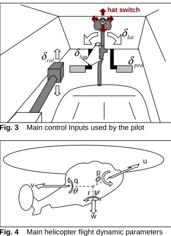
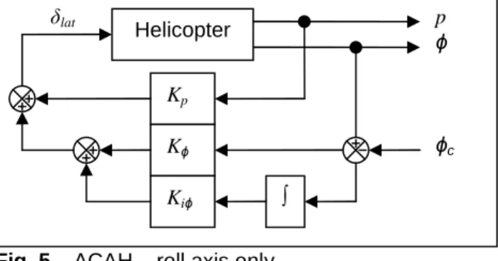
On Fig. 3 the main control inputs used by helicopter pilots are presented. The Fig. 4 shows the main dynamical variables used to represent the flight dynamics of a helicopter. Tab. 1 lists the parameters used for the establishment of the state space representation of the natural system.

Tab. 1 List of main parameters

δcol Collective input /1 δlat Lateral cyclic input /1 δlon Longitudinal cyclic input /1 δped Pedals input /1

u Longitudinal speed m/s

v Lateral speed m/s

w Vertical speed m/s

p Roll rate rad/s

q Pitch rate rad/s

r Yaw rate rad/s

ɸ Bank angle rad

θ Pitch angle rad

Ψ Heading angle rad

2.2 Basis of piloting a helicopter

The collective stick is connected to the swash-plate and permits the control of the rotor lift force magnitude by modifying the average component of the blades pitch angle. The cyclic stick allows changing the 1-per-rev harmonics of the blades pitch angle, and thus controlling the roll and pitch moments of the rotor. This results in the orientation of the rotor around its roll axis when acting on the lateral cyclic input, and on the pitch axis when acting on the longitudinal cyclic input. The pedals allow the

control of the anti-torque (or tail) rotor, and the motion of the helicopter around its yaw axis.

Fig. 3 Main control Inputs used by the pilot

Fig. 4 Main helicopter flight dynamic parameters 2.3 State Space representation of a

helicopter

The establishment of this kind of representation is well known [7] [8]. Let U, X, and Y respectively be the input, state and output vectors of the state space representation of a helicopter. Then, the inputs and the states of the helicopter are:

(1)

[

]

[

]









=

=

t t ped lon lat col

r

q

p

w

v

u

X

U

ψ

θ

φ

δ

δ

δ

δ

,

,

,

,

,

,

,

,

,

,

,

Moreover, A, B, C, D are respectively the state, command, observation and input/output matrices. Using usual linear assumptions around equilibrium, they can be calculated from full representative nonlinear flight dynamic models or identified from dedicated flight tests. In this study, authors have used HOST© (Helicopter Overall Simulation Tool [9]), a modelling and simulation tool developed by Airbus Helicopters, and jointly improved by ONERA. (2)

A

∈

M

_9x9

B

∈

M

_9x4

C

=

I

_9x9

D

=

0

_4x9 HQ test good Implementation Tuning bad p u

φ

q

θ

v r

ψ

w hat switch col

δ

lat

δ

lon

δ

ped

δ

Design and tuning process HQ specifications Implementation

Then, we can write the state space representation of the helicopter (3). (3)







=

+

=

X

Y

U

B

X

A

X

&

.

.

This 9-by-9 linear model has been used for the development of a process aiming to integrate HQ requirements from the early phase of gains design. The control law studied during this work was an Attitude Command Attitude Hold (ACAH) control strategy

2.4 Attitude Command Attitude Hold (ACAH) control law

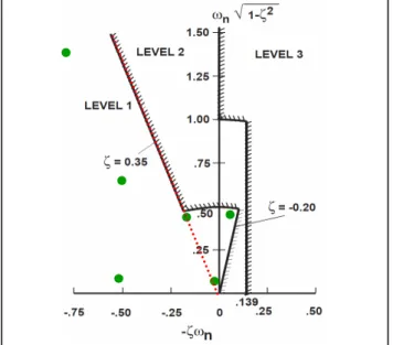
The Attitude Command Attitude Hold (ACAH), as shown on Fig. 5 for the roll axis as an example permits to control the attitudes of the helicopter (ɸ for the roll axis), governed by the pilot cyclic stick.

Fig. 5 ACAH – roll axis only

Then, we can write the feedback equation for this axis (4).

(4)

δ

lat

=

K

p

.

p

+

K

φ

.(

φ

−

φ

c

)

+

K

iφ

.

∫

(

φ

−

φ

c

)

The aim of this paper is to set up a method to help designers in tuning the gains of the ACAH control law, taking into account HQ requirements as described in the ADS-33 standards. Only some of these criteria have been selected for this study and are presented in the next subsection.

2.5 Selected criteria from ADS-33 (all others MTE – hover and low speed)

The standard specifies HQ criteria for a wide range of helicopters. All criteria depend on the case study, and they are detailed in a specific classification. For this paper, we will focus on a specific case study, explained hereafter.

2.5.1 The case study

The helicopters are indexed into 4 rotorcraft categories: attack, scout, utility and cargo. This paper will focus on the study of a 10-ton class helicopter: cargo-type. A table in the standard specifies which Mission Task Elements (MTE) the studied helicopter should be capable of, and the required agility needed for each one. For this paper, we will focus on the “all others MTE” requirements only. We will focus on the “hover and low speed” case.

A rating of Usable Cue Environment (UCE: 1, 2 or 3) is provided. We will study the case of UCE 2, which means that the pilot “can make limited

corrections with confidence and precision is only fair” [2] on attitude and / or translational piloting.

This can be evaluated using a Visual Cue rating scale (provided in the standard as well). Depending on the case study, a table specifies the required response type. Here, the ACAH is needed to be able to achieve Level 1 response type rating. The bloc diagram previously presented corresponds to this response-type requirement.

The next sections will explain the requirements for this case study. The roll axis will be focused. The three selected criteria are eigenvalues placement (Section 2.5.2), attitude quickness placement (Section 2.5.3) and bandwidth / phase delay placement (Section 2.5.4). They respectively evaluate the helicopter’s stability, agility and ability to follow high frequency inputs with accuracy. They constitute the basic quantitative criteria to evaluate the expected overall Handling Qualities (HQ) of a helicopter. The standard explains how to calculate and plot the requirements for each criterion. The aim is to place the resulting point(s) calculated for each criterion in the “LEVEL 1” area on its associated plot. “LEVEL 2” area is an indicator of “medium” quality. “LEVEL 3” area should be avoided. “The rotorcraft

shall meet the Level 1 standards for all criteria. Violation of any one requirement is expected to degrade Handling Qualities” [2]. The bold black lines

on Fig. 6, 8 & 10 represents a limit between two areas. The green points on each of these plots are examples of good tunings, for its associated criterion.

2.5.2 Limits on oscillations: stability criterion This criterion is evaluated by calculating the eigenvalues of the dynamic matrix of the linearized closed loop system. The requirements for their positioning, as shown on Fig. 6, determine the quality of the helicopter stability. The Level1/Level2 limit can be sufficiently approximated by ζ=0.35 (red

dotted line on Fig. 6). ɸ p Kp Kɸ Kiɸ ∫ ɸc δlat Helicopter

Fig. 6 Stability criterion: pole placement

2.5.3 Requirements for moderate amplitude attitude changes: quickness criterion This criterion is evaluated using attitude capture flight tests. For the gain tuning studies, attitude change simulations are performed. The criterion is computed using 3 parameters (Fig. 7): peak roll rate (ppk), peak roll change (∆ɸpk) and minimum roll

change (∆ɸmin). Then, 2 of these 3 parameters are

used to calculate the quickness criterion (Q). The requirement for its positioning depending on the minimum attitude change is shown on Fig. 8. The Level 1 / Level 2 limit can be approximated by (red dotted curve on Fig. 8):

(5)

b

a

k

p

Q

pk pk

₊

+

∆

=

∆

=

min

θ

φ

with k = 31deg/sec, a = 17deg and b = 0.22/sec

2.5.4 Requirements for small-amplitude roll attitude changes: accuracy criterion This criterion is evaluated using frequency sweeps capture flight tests. In this paper, Bode diagrams are generated using either equivalent linear models of the closed loop system, if available, or using directly frequency sweep simulations. For the study of the ACAH, this criterion is performed using 3 parameters, as detailed on Fig. 9: the bandwidth ω180 defined by a cut-off of the phase at -180°, the bandwidth phase ωBWphase using a +45° phase margin

from ω180 cutoff, and the variation of phase ∆ɸ2ω180

from -180° at the frequency 2*ω180. Then, these 3

parameters are used to calculate the phase delay parameter (τp), as defined on Fig. 9. The

requirement for positioning τp depending on ωBWphase

is shown on the next figure: Fig. 10.

Fig. 7 Definition of the attitude quickness parameters during an attitude change

Fig. 8 Quickness criterion: attitude quickness

Fig. 9 Definition of small amplitude criterion parameters

qpk (ppk) [rpk]

Fig. 10 Accuracy criterion: bandwitdth / phase delay The Level 1 / Level 2 limit can be approximated by a vertical line at ωBWphase=2rad/sec (red dotted line on

Fig. 10). Indeed, the values of phase delay (τp) seem

to be mainly influenced by the natural system delays. The gains of the control laws seem to have negligible influence on its value [10], for stabilized systems at least.

2.6 Description of the procedure developed at ONERA

The first idea followed in order to establish a “direct method of tuning” was to use the sensitivities of gains to the criteria as design guidance for full linearized systems. A tool (CAST-HEL-AP: Computer Aided Setting and Tuning tool for Helicopters’ Autopilots) was developed at ONERA Salon de Provence for this purpose [10]. The advantage of this procedure is: the designer is not influenced by an optimization tool that could trap his design in a local optimum.

However, due to the non-linearity of the relationship between the gains and the HQ criteria, the sensitivity method can’t be efficiently applied if the initial set of gains doesn’t already insure the stability of the helicopter with a significant improvement of the overall FQ This means that to be fully efficient with the sensitivity analysis toolbox (CAST-HEL-AP), there is a need to set up a process of gains initialization providing already fair handling qualities. This paper focuses on the establishment of the methodology to initialize the gains of a control law with FQ objectives.

The final full procedure focused by ONERA is summarized on Fig. 11.

The section 3 will focus on the explanation of the new linear initialization process (yellow part on the Fig. 11).

The section 4 will give an example of a complete design and evaluation, using the full procedure. 3. PROCESS FOR INITIALIZING GAINS OF

CONTROL LAWS WITH FQ OBJECTIVES As shown on Fig. 11, the idea is to create a process that will permit to initialize the gains of the control law, directly from a set of FQ criteria, specified at the beginning of the design studies. If the requirements chosen to be achieved are too restrictive, there is a risk of saturation from actuators. Then, the aim is to achieve sufficient levels of quality for the whole set of requirements, not to improve them more than needed.

The helicopter is complex (hard coupled system), the constraints from the control laws are hard (non-full state feedback) and the requirements from the standard are very specific (non-common). Therefore, it was decided to establish simplified models of the open loop and the closed loop system. As it is explained thereafter, these models can be used to help in establishing the initialization process.

The methodology is exposed through the example of the tuning of the ACAH control law for the roll axis. The criteria chosen as design objectives are those exposed in section 2.5 for the study of a 10T class helicopter, cargo-type, with UCE2-type and all other MTE-type requirements. As for an initialization process – with sufficient FQ requirements – the linear models will ignore actuator models and their saturations.

Fig. 11 Full procedure of tuning focused by ONERA HQ targets

Analyzes and charts

Gains initialized

Implementation of gains

on full linear model with CAST-HEL-AP Expected HQ Evaluation of the linear initialization process Adjustments of gains on

full linear model with CAST-HEL-AP using linear

sensitivities results

Implementation of gains

on full nonlinear model Gains and expected

HQ improved

Obtained HQ

Adjustments of gains on

full nonlinear model using

local linear sensitivities

Evaluation of the linear sensitivities process

Final gains and HQ

Evaluation of the full procedure Evaluation of the initialization of the final system

3.1 Analytical studies led to help establishing relationship between gains and FQ criteria

Each axis-control law is created for specific purposes, say for specific control of the axis. The main aim of a control law for one axis is not to control the other axes, which are stabilized thanks to their own axis-control laws (or by the pilot at least). Then, the work made for one axis can be re-used for the other axes. Thanks to these conditions, and due to the complexity of the system, we will consider the establishment of a simplified one-axis open loop (and closed loop) system.

3.1.1 Simplified one-axis open-loop model The axis chosen to be studied here is the roll axis. The associated states are (p,ɸ). The main input used to pilot this axis is δlat. Then, from (1), let X1, X2, U1

and U2 be: (6)

[ ]

[

]

[ ]

t

[

]

t t ped lon col t lat

r

q

w

v

u

X

p

X

U

U

ψ

θ

φ

δ

δ

δ

δ

,

,

,

,

,

,

,

,

,

2 1 2 1

=

=

=

=

Then (3) can be written on another way using permuted matrices of A and B, such that:

























+

























=

















2 1 22 21 12 11 2 1 22 21 12 11 2 1

.

.

U

U

B

B

B

B

X

X

A

A

A

A

X

X

&

&

(7)

X

&

₁

=

A

₁₁

.

X

₁

+

A

₁₂

.

X

₂

+

B

₁₁

.

U

₁

+

B

₁₂

.

U

₂ (8)

X

&

₂

=

A

₂₁

.

X

₁

+

A

₂₂

.

X

₂

+

B

₂₁

.

U

₁

+

B

₂₂

.

U

₂

Then, some hypotheses can be used for the establishment of our simplified models.

- Hypothesis 1: X2 = 0. During a roll change, the

pilot or the other control laws take care of the stabilization of the other axes (vertical, pitch, yaw). We consider the associated states will only slightly vary from equilibrium, say zero. - Hypothesis 2: U2 = 0. To pilot the roll axis, the

mainly used input is the roll associated input. For an initialization of gains procedure, even if slight variations of the other inputs are needed to compensate couplings, we consider that the other inputs do not vary from initial equilibrium, say zero.

Applying these two hypotheses on (7) imply: (9)

X

&

₁

=

A

₁₁

.

X

₁

+

B

₁₁

.

U

₁

- Hypothesis 3:

φ

&

= p. The derivative of the roll angle is approximated to the roll rate (true while in pure lateral flight, and this fits with the conditions of the associated evaluations of ADS33 requirements).

Applying this new hypothesis, using the definitions from (6) and using sensitivities Lp=∂(ṗ)/∂(p),

Lɸ=∂(ṗ)/∂(ɸ), Lδlat=∂(ṗ)/∂(δlat), (9) becomes:

(10)

p

&

=

L

_p

.

p

+

L

_φ

.

φ

+

L

_δlat

.

δ

_lat

- Hypothesis 4: Lɸ = 0. The dynamic between the roll angle and the derivative of the roll rate is neglected (negligible value compared with the other sensitivities: usually less than 10-9%). Applying this hypothesis on (10) implies: (11)

p

&

=

L

_p

.

p

+

L

_δlat

.

δ

_lat

3.1.2 Simplified one-axis closed-loop model Including the equation of the control law (4) into (11), we obtain:

(

+

−

+

∫

−

)

+

=

L

_p

.

p

L

_lat

K

_p

.

p

K

.(

_c

)

K

_i

(

_c

)

p

&

_{δ φ}

φ

φ

_φ

φ

φ

Using hypothesis 3 again, and applying Laplace transformations (s is the Laplace variable here), this last equation can be written:

(12)

(

)

s

L

L

s

L

s

p l c l c

φ

φ

φ

φ

φ

φ

.

=

ˆ

.

.

+

δ1

.

−

+

δ2

.

−

2 (13) with:











=

=

+

=

φ δ δ φ δ δ δ i lat l lat l p lat p p

K

L

L

K

L

L

K

L

L

L

.

.

.

ˆ

2 1

Then, the input/output transfer function is:

(14)

(

)

2 1 2 3 2 1

.

.

ˆ

.

l l l l c

s

L

s

L

s

L

L

s

L

δ δ δ δ

φ

φ

−

−

−

+

−

=

We obtain an order three model. By analogy to the usual natural modes of the rotorcraft, we choose to impose one real mode and two complex modes to the behaviour of the closed loop model. Then, (14) can be written with an equivalent transfer function:

(15) ₂ 2 2 1 2

.

.

.

2

.

1

.

1

n n n c

s

s

s

s

ω

ω

ζ

ω

τ

τ

φ

φ

+

+

⋅

+

+

=

with: (16) n

ω

ζ

τ

τ

2

=

1

+

2

.

and ωn > 0, τ1 > 0, τ2 > 0, ζ > 0

A relation between the parameters of the equivalent transfer function and the associated gains of the one-axis piloting assistance can be established (17).

(17)































₊

+

−

=

+

−

=

−

=

lat n lat p p lat n n lat n i

L

L

L

K

L

K

L

K

δ δ δ φ δ φ

τ

τ

ω

ζ

τ

ω

τ

ω

ζ

τ

ω

.

.

.

.

2

1

.

.

.

.

2

.

1 1 1 2 1 1 2

Thanks to these developments, (17) is specifically very interesting. Indeed, if values of ωn, τ1 and ζ can

be chosen, the gains of the simplified model can be directly initialized with (17), using the sensitivity parameters Lp and Lδlat from the model. Then, the idea is to choose the values of the parameters of the equivalent transfer function in order to satisfy sufficient FQ requirements. A tool can help in that purpose.

3.2 Development of a tool generating charts of FQ for simplified models of helicopters This tool has the aim to help the designer in choosing values of the parameters of the simplified models such that the associated set of expected FQ are sufficiently good. The idea for this tool is to generate the criteria for a sweep of models such that the parameters used in (15) (ωn, τ1 and ζ) are

physically suitable. Then, the data can be used to generate charts of FQ. The designer can then use these charts to find associated values of ωn, τ1 and ζ

such that the expected FQ are those recommended by the standard. Then the equations from (17) permit the initialization of the gains. The first step is to establish a range of values of ωn, τ1 and ζ

physically suitable to the system. A quick overview on (15) can help in this. On the one hand, if ωn, τ1 or

ζ are almost equal to zero, the model (15) might change radically (risk of creation of a pure unstable integrator for example). Furthermore, the impact on the values of the gains (17) can be unacceptable (value of Kiɸ can tend to infinity for example). On the

other hand, because we are studying a physical and pilotable system, the maximum values of ωn, τ1 and ζ

can be empirically limited. Finally, one can choose to generate a set of models such as (15) with:

(18)











<

<

<

<

<

<

1

1

.

0

3

1

.

0

3

1

.

0

1

ζ

τ

ω

n

Then, all criteria can be calculated for the whole set of models using fast linear simulations.

Here is an example of an algorithm for generating charts of FQ:

- Choose a value for ζ and a value for the amplitude of the attitude change ɸc (necessary

for attitude quickness calculations).

- For ωn from 0.1 to 3 and for τ1 from 0.1 to 3 do:

- Create the simplified transfer function (15) (using (16)).

- Calculate the attitude quickness parameters using a linear attitude change simulation. - Calculate the bandwidth / phase delay

parameters using a phase Bode diagram. - Calculate isopleths of attitude quickness and

bandwidth / phase delay parameters.

- Calculate isopleth of the approximated Level 1 / Level 2 limit for the attitude quickness criterion (Fig. 8 and equation (5)).

- Calculate isopleth of the approximated Level 1 / Level 2 limit for the bandwidth / phase delay parameter (Fig. 10).

- Plot the whole set of isopleths in a chart with ωn

depending on τ1.

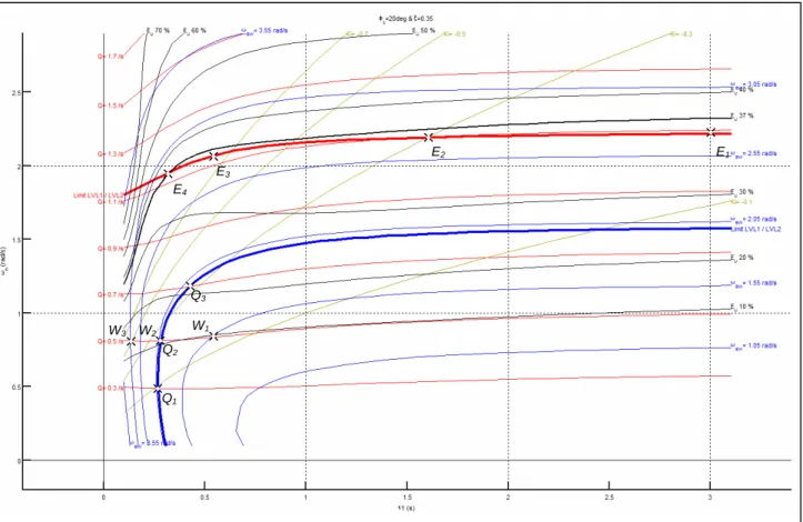
3.3 Explanation of how to read a chart through an example

The Fig. 12 shows an example of a chart of FQ using the previous algorithm, choosing ζ=0.35 and ɸc=20deg, for the roll axis. A model of natural delays

is included in the calculations. A point on this figure is defined by specific values for ωn and τ1. As ɸc and

ζ are fixed, then a point defines a model such as (15). For each point, all criteria and interesting parameters are generated as explained in previous sections. Then, for each point on this figure, we have information on the behaviour of the simplified one-axis model of the helicopter, for the roll axis in this example.

The coloured lines plotted are isopleths of criteria and parameters of interest for this paper. For example, the red bold line represents all models possible to choose if we want to be sure that their performance in terms of quickness is at the LEVEL 1 / LEVEL 2 limit (as defined by the red dotted line on Fig. 8). This means that if we chose a point on this line, the associated parameters ζ, ωn and τ1 (and ɸc)

generate a model (15) which insures to provide a quickness level verifying equation (5), for this case study (ɸc).

The example for the red bold line is the same for the blue bold line: if we choose a model on this line, the associated parameters insure that the simplified model presents a sufficient LEVEL 1 quality with respect to the bandwidth criterion (as defined by the red dotted line on Fig. 10).

Fig. 12 Example of a chart generated for the roll axis control law of a cargo-type helicopter All the coloured lines follow the same rule. Red lines

give information on quickness (isopleths of Q

parameter). Blue lines give information on bandwidth (isopleths of ωBW parameter). Yellow lines are isopleths of the integral gain Kiɸ (used later in the

communication). Black lines give information about the need on actuator energy during the attitude change simulation made to calculate the attitude quickness, using an energetic criterion (explained in next subsection). Then, for each point on this chart, a model and its associated FQ are generated and plotted (via isopleths).

One can choose a point on this kind of chart, depending on its FQ objectives. Then thanks to (17), one can calculate the associated gains that will permit to obtain sufficient FQ levels – for the simplified model at least. These gains can be used as initialization for the complete model.

The differences between the results of the chart and those obtained with full linear models are evaluated in the next sections so that the designer has information on the results he can trust in. The points on Fig. 12 will mainly be used for these evaluations. 3.4 Additional criterion for energy evaluation During an attitude change simulation, an amount of energy is used from the actuators. In order to evaluate this amount of energy spent, a criterion can

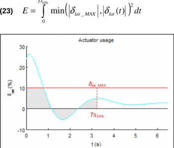
be used. We will check the energy used until the system will be considered as stabilized, so that the energy usage will be stabilized as well. We decided to consider that a system modelled such as (15) is stabilized once the values of the attitudes do not extend any more over a band of 10% of the final value.

The instant from when the system is stabilized is called settling time to 10%: Ts10%. To evaluate this

settling time, the model (15) can be approximated by (19). (19) ₂ 2 2

.

.

.

2

n n n c

s

ζ

ω

s

ω

ω

φ

φ

+

+

≈

The Fig. 13 shows a usual attitude change simulation generated with (15) in cyan, and its associated approximated attitude change simulation generated with (19) in blue. The time expression of the envelope of the time response of the model (19) to a step input ɸc can be approximated by (20) (red

curve on Fig. 13). (20)

_















−

−

≈

− 2 . .

1

1

.

)

(

ζ

φ

ζω φ t c n

e

t

Env

E4 E2 E3 Q1 Q2 Q3 W1 W2 W3 E1

Fig. 13 Evaluation of the approximated settling time to 10%.

Finally, we can calculate the settling time to 10% of the final value:

(21)

_















−

−

≈

=

− 2 . . % 10

1

1

.

95

.

0

)

(

% 10

ζ

φ

φ

ζω φ Tr c c n

e

Tr

Env

(22)

(

)

n

Tr

ω

ζ

ζ

.

1

05

.

0

log

2 % 10

−

−

≈

Thanks to all data generated, it is now possible to evaluate the amount of energy used during an attitude change simulation (Fig. 14) using the E

criterion (applied to the roll axis):

(23)

=

∫

(

)

% 10 0 2 _

,

(

)

min

Tr lat MAX lat

t

dt

E

δ

δ

Fig. 14 Evaluation of the energy used during an attitude change simulation (model (15))

The value of δlat_MAX corresponds to the value of

static saturation of actuators. The criterion E can be visualized with the grey area on Fig. 14. Its value will be compared to the maximum of energy the actuator could furnish during the same time. This can be evaluated thanks to the Ue criterion:

(24)

=

∫

(

)

% 10 0 2 _ Tr MAX lat

dt

Ue

δ

Finally, the energy criterion chosen to be considered for the tuning will be expressed as a percentage of the maximum amount of energy the actuator could have generated during the attitude change simulation until the settling time to 10%. This criterion will be called Energy Usage Eu (%):

(25)

Ue

E

Eu

=

100

⋅

Isopleths of Eu have been plotted on Fig. 12. If Eu tends to 100%, this means the actuator saturates during the whole attitude change. Then the designer might look for minimizing its value. Later, a (realistic) filter will be used so that the first peak of the actuator usage can be highly reduced, with no significant loss on overall expected FQ. By the way, for more security about saturations due to windups, an anti-windup architecture could be used [11].

3.5 Evaluation of the chart

Many points of tuning have been chosen on Fig. 12 in order to check the reliabilities of the expected FQ. Full linear simulations (including natural system delays and actuator models) have been led in that purpose (using CAST-HEL-AP [10]). The results are summarized on Fig. 15, 16 & 17:

- red dots for the expected results with chart. - blue stars for the obtained results with full linear

simulations, using same gains.

- black, green and grey squares for full linear and nonlinear design led in section 4.

The points Q1, Q2 and Q3 have been chosen such that the expected bandwidth is at the Level 1 / Level 2 limit. The points W1, W2 and W3 have been chosen such that the expected quickness parameter is at Q=0.5. The points E1, E2, E3 and E4 have been chosen such that all expected criteria are at least at the Level 1 / Level 2 limits. Results are summarized in Tab. 2.

The quickness parameter is expected (simplified model) to be improved by 40% between Q1 and Q2 and by 29% between Q2 and Q3. The obtained results (full linear model) show that they are improved by 23% and 19%.

Ts10% δlat_MAX

Fig. 15 Attitude quickness results (i = {1:4})

Fig. 16 Bandwidth / phase delay results (i = {1:4})

Fig. 17 Poles results (i = {1:4})

Tab. 2 Summary of the results and comparison (Gap row) between simplified and full linear models

Points on Fig. 12 Q1 Q2 Q3 W1 W2 W3 E1 E2 E3 E4 τ1 (s) 0.27 0.28 0.45 0.52 0.28 0.13 3 1.6 0.56 0.32 ωn (rad/s) 0.49 0.81 1.18 0.82 0.81 0.81 2.22 2.19 2.08 1.94 Q (/s) 0.3 0.5 0.7 0.5 0.5 0.5 1.08 1.10 1.15 1.18 Simplified model ωBW (rad/s) 2 2 2 1.55 2 3.05 2.69 2.72 2.75 2.84 Q (/s) 0.5 0.65 0.8 0.65 0.65 0.7 1.15 1.2 1.25 1.35 ωBW (rad/s) 1.85 2.1 1.8 1.4 2.1 4.7 2.4 2.45 2.55 2.95 Full linear model ζ 0.25 0.3 0.25 0.2 0.3 0.35 0.2 0.2 0.25 0.3 ∆Q% -40% -23% -13% -23% -23% -29% -6% -8% -4% -6% ∆ωBW% +8% -5% +11% +11% -5% -35% +12% +11% +8% -4% Gap ∆ζ% +29% +14% +29% +43% +14% +0% 43% 43% 29% 14% Kp -0.17 -0.19 -0.13 -0.056 -0.19 -0.86 0.013 -0.017 -0.11 -0.27 Kɸ -0.14 -0.25 -0.35 -0.176 -0.25 -0.62 -0.54 -0.58 -0.63 -0.8 Gains Kiɸ -0.083 -0.21 -0.36 -0.128 -0.21 -0.64 -0.16 -0.3 -0.67 -1.2

The bandwidth parameter is expected to be improved by 22% between W1 and W2 and by 34%

between W2 and W3. The full linear simulations show respectively an improvement of the bandwidth by 33% and 55%. Then, in each case, the sensitivity is verified.

It comes out from Tab. 2 that in each case, the overall FQ obtained with the full linear model are in an area near the expected FQ given by the chart. This result demonstrates that the gains generated by the charts are able to achieve the targeted FQ criteria.

As a consequence, the charts seem to be enough accurate to permit a fast and efficient initialization of the gains with multiple FQ objectives.

3.6 Advices for using the chart in order to initialize the gain tuning process with HQ objectives

In order to meet LEVEL 1 HQ, a designer might want to use a chart for his design. The first step is to choose the case study. Depending on this case study, the set point might be fixed, and, in order to meet sufficient LEVEL 1 stability, ζ might be fixed to

0.35. Then, thanks to the algorithm, a chart can be generated. The Fig. 12 has been generated using the recommendations from the standard with ɸc=20deg and ζ=0.35.

In order to meet sufficient LEVEL 1 quality for bandwidth phase delay criterion, a point might be chosen on the blue bold line. However, if a point is chosen on this line, the associated quality for

Q1 Q2=W2 Q3 W1 W3 E1 E2 E3 E4 Qi W2 W1 Ei W3 E4’ E4’’ E4’’’ W2=Q2 Q3 E2 E3 E4 W3 Wi & Q2 Q3 Ei Q1 Q1 E1 W1 E4’ E4’’ E4’’’ Q3 W2=Q2 Q1 W1 W3 E1 E2 E3 E4 Q1 Wi & Q2 Q3 E1 E2 E3 E4 E4’=E4’’ E4’’’

attitude quickness is never at LEVEL 1 for this case study. None of these designs seem interesting to meet good overall FQ.

Then, the designer might choose a point on the red bold line. Indeed, all points on this line generate gains with which the expected quality for attitude quickness is sufficiently at LEVEL 1. Furthermore, the expected quality for bandwidth phase delay is at LEVEL 1 with a large expected margin. Then, if a designer chooses any point on this line, the overall expected FQ might be at LEVEL 1.

A question might appear then: if any point can be chosen on the red bold line (for example E1, E2, E3 and E4), which can be considered as the best? Indeed, the expected FQ objectives seem sufficiently good in all cases. Here, we suggest considering two additional criteria for the initialization procedure: an energy criterion (the energy usage criterion explained before) and a new uncoupling criterion.

The black isopleths on Fig. 12 already give indications on the expected amount of energy used for each design during the attitude change simulation done to generate the attitude quickness, as explained in section 3.4. We suggest minimizing this criterion (in order to minimize the risks associated with potential saturations). Then, in this case study, the left area of this chart might be avoided.

The last objective might be to minimize the coupling of the full system. Eventually, even if the model we established has been simplified for a one-axis study, the coupling of the system can be seen by this model as perturbations.

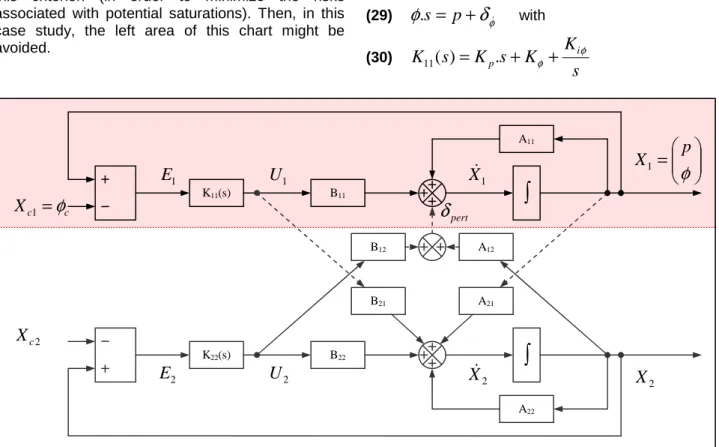
Indeed, the equations (7) and (8) can be seen schematically on Fig. 18, using a framework similar to the individual channel design [12]. In section 3.1,

U2 and X2 have been neglected such as our model

has been reduced to the red part of Fig. 18. However, these hypotheses are wrong. Then, we can see these coupling signals as perturbation δpert from the point of view of the one-axis control law. Then, if we wish to consider these couplings during the tuning process, (9) becomes:

(26)

X

&

₁

=

A

₁₁

.

X

₁

+

B

₁₁

.

U

₁

+

δ

_pert with

(27)

_















=

φ

δ

δ

δ

& &p pert

Then, using hypothesis (3), using Laplace transformations and considering ɸc=0, (26) and (27)

become:

(28)

p

.

s

=

L

_p

.

p

+

L

_δlat

.

K

11

(

s

).

φ

+

δ

_p& and (29)

φ

.

s

=

p

+

δ

_φ& with (30)

s

K

K

s

K

s

K

₁₁

(

)

=

_p

.

+

_φ

+

iφ

Fig. 18 Helicopter architecture with the usual ACAH control law

K11(s) B11 A11

∫

K22(s) B22 A22

∫

B21 B12 A12 A21 2

X

1

X

&

1

E













=

φ

p

X

₁ 2 c

X

c c

X

₁

=

φ

2

E

1

U

2

U

X

&

₂ pert

δ

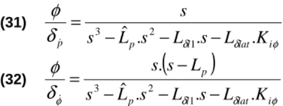
Finally, the new transfer functions between each one of the perturbations and ɸ are:

(31) φ δ δ

δ

φ

p

s

L

p

s

L

l

s

L

lat

K

i

s

.

.

.

ˆ

1 2 3

−

−

−

=

& (32)

(

)

φ δ δ φ

δ

φ

i lat l p p

K

L

s

L

s

L

s

L

s

s

.

.

.

ˆ

.

1 2 3

−

−

−

−

=

&

Then, thanks to the control law, the steady state error to step input like perturbations is zero. Indeed:

(33)

lim

(

)

lim

.

(

)

0

0

=

=

=

→ ∞ →

t

s

s

s

t s

ϕ

φ

ε

But the steady-state errors to ramp-like perturbations are respectively (using normalized amplitudes): (34) φ δ φ

ϕ

φ

ε

i lat s t p s

K

L

s

s

t

.

1

)

(

.

lim

)

(

lim

0 _

=

=

=

−

→ ∞ → & (35) φ δ φ φ

ϕ

φ

ε

i lat p s t s

K

L

L

s

s

t

.

)

(

.

lim

)

(

lim

0 _&

=

_→∞

=

_→

=

The results from (34) and (35) are crucial for decoupling objectives. Indeed, as required by the standard, the tuning must be led by keeping in mind to uncouple the system as much as possible. Here, we can see that we tend to help in that uncoupling by increasing the value of the integral gain. That’s why the isopleths of Kiɸ have been plotted on Fig. 12

(yellow lines). Here is the full procedure advised for an efficient initialization of the gain tuning process: - Choose a case study in order to fix the FQ

objectives as well as ζ and ɸc.

- Generate the chart for this specific case study of the one axis control law.

- Find the area in which the expected attitude quickness and bandwidth phase delay criteria are both at LEVEL 1 (this should be near at least one of the two bold lines, red or blue on Fig. 12). - Choose a point in this area, near at least one of these limits, by making a compromise between maximizing as much as possible the integral gain (for uncoupling) and minimizing as much as possible the energetic criterion during the one-axis attitude change simulation led.

4. APPLICATION AND EVALUATION OF THE FULL PROCEDURE

The initialization of gains procedure is applied to the full helicopter, for each axis. Then, an analysis is led for the roll axis only (without modifications of the gains on pitch and yaw). All results obtained during the analyses led for the roll axis in this section are summarized on Tab. 3. All FQ obtained in this section are represented on Fig. 15, 16 & 17: red dot

Ei (with i=4) for expected FQ from the chart, blue star E4 for obtained FQ with same gains used on full linear model, black square E4’ for the FQ obtained after modifying the gains on full linear model using local linear sensitivities, green square E4’’ for the FQ obtained with the same gains used on the full non linear model, E4’’’ for the final FQ obtained on full non linear model after modifying the gains using local linear sensitivities. All these steps match with the full procedure explained by Fig. 11.

All FQ objectives are those explained in section 2.5, for the roll axis.

4.1 Initialization of the gains of the full linear model using charts

Here, we directly apply the initialization of gains procedure explained in section 3.6. We choose to tune the ACAH for the roll axis with LEVEL 1 FQ objectives. We fix: ζ=035 and ɸc=20deg. The chart on

Fig. 12 has been generated with these conditions. A point on the red bold line generates gains with which all expected FQ are at least sufficiently in the LEVEL 1 area: we will choose a tuning on this line. A good compromise between reducing energy consumption (black isopleths of Eu criterion) and increasing uncoupling (yellow isopleths of Kiɸ criterion) can lead

to choose the point E4: red dot Ei for i=4 on Fig. 15, 16 & 17. The expected FQ and the associated gains are summarized on the first row of Tab. 3. The Fig. 15, 16 & 17 show that the overall expected FQ with the simplified model are quite well verified with the full linear model (blue star E4). Indeed, the gains obtained with the chart have been implemented in CAST-HEL-AP [10] to evaluate the FQ (using exactly same conditions) with the full linear model: this includes model of actuators and natural system delay. The results are summarized in the second row of Tab. 3.

Tab. 3 Summary of the results of the full tuning procedure: last three columns show the evolution of gains

Full tuning procedure Q (/s) ωBW(rad/s) ζ Kp Kɸ Kiɸ

Expected FQ from chart and associated gains 1.18 2.84 0.35 -0.27 -0.8 -1.2

Obtained FQ with full linear model (same gains) 1.35 2.95 0.3 -0.27 -0.8 -1.2 Modifications of the gains using sensitivities (full linear model) 1.28 3.08 0.35 -0.3 -0.8 -1.2 Modified gains Implemented on the full non-linear model 1 2.1 0.35 -0.3 -0.8 -1.2 Modifications of the gains on the full non-linear model 1.2 2.7 0.45 -0.3 -1.2 -1.2

The last column of Tab. 2 gives precisions about the gaps of results between the expected FQ with simplified model and the obtained FQ with full linear model. There is a gap of 6% between the results of quickness, 4% between the results of bandwidth and

14% between the results of stability. This confirms the overall obtained FQ with full linear model are in the area of the overall expected FQ by the chart. 4.2 Modification of the gains of the full linear

model using linear sensitivities

The blue star E4 on Fig. 17 indicates a lack of stability for the full linear model with these gains. Using local linear sensitivity results [10], the derivative gain is increased in order to obtain LEVEL 1 stability for the associated slow mode. The results are summarized with the third row of Tab. 3 and with the black square E4’ on Fig. 15, 16 & 17.

Thanks to this modification, the overall expected FQ with full linear model are at LEVEL 1 for all criteria. In order to obtain these results, only the derivative gain has been increased by 10% only. Doing this, the quickness parameter has been decreased by

5%, the bandwidth has been increased by 4% and the stability has been increased by 14%.

All of this means that we have initialized the gains efficiently in one step thanks to the chart. The sensitivities results are used only to make slight adjustments at this step. Now, all expected FQ are all in LEVEL 1 area, with a good margin for the bandwidth (as it was already expected by the chart). 4.3 Evaluation of the differences of results

between full linear models and full nonlinear models

Then these gains are used with full nonlinear models (including actuator model and natural system delay) to evaluate the overall FQ, using exactly same conditions: results are summarized with the fourth row of Tab. 3 and with green square E4’’ on Fig. 15, 16 & 17.

As we can see, the quickness falls by 28% and the bandwidth falls by 47% (the stability is evaluated with full linear model, that’s why there is no modification on this criterion). The figures show that the bandwidth is still in the LEVEL 1 area. Only the quickness is in the LEVEL 2 area. However, the overall obtained FQ are still in an interesting area, as expected by linear results.

4.4 Modifications of the gains on the full nonlinear model using linear sensitivities results

The green square E4’’ on Fig. 17 indicates a lack of quickness for the full nonlinear model. Using local linear sensitivities results, the proportional gain is increased in order to obtain LEVEL 1 quickness. All results are summarized with the fifth row of Tab 3. and with grey square E4’’’ on Fig. 15, 16 & 17. Then, by increasing the proportional gain by 33%, the quickness has been increased by 17%, the bandwidth has been increased by 22% and the stability (obtained with full linear model) by 22%. The overall expected FQ is at LEVEL 1.

4.5 Evaluation of the full direct process: comparison of expected results from charts with obtained results from full nonlinear model

The aim was to tune the gains of the control law of the helicopter in order to obtain LEVEL 1 expected HQ for the roll axis. More precisely, there were conditions on quickness, bandwidth and stability parameters. Some gains have been chosen for initialization. Then, in order to meet LEVEL 1 limits, the derivative gain has been increased by 10% and the proportional gain by 33%. During the tuning process, the quickness parameter has been increased by 2%, the bandwidth parameter has been decreased by 5% and the stability parameter has been increased by 22%.

Finally, with this “direct” procedure, the overall expected HQ has been set to LEVEL 1, in few steps, using the FQ requirements from ADS-33. Only slight adjustments have been necessary.

5. CONCLUSION

ONERA has been working for several years to the establishment of an efficient methodology of gain tuning for helicopter control laws with Handling Qualities objectives, from the early steps of gains design. In this paper, an example of the full procedure has been presented.

Thanks to the methodology developed, the use of Flying Qualities charts generated from an analytical study widely contributes to an efficient initialization of control law gains constrained by Flying Qualities requirements. Moreover, the physical basis of these charts insures not only the initialization of the gains, but also a correct sensitivity of the gains to the Flying Qualities criteria, as well as a good estimation of tuning points near the limits. A tool implementing all this methodology is currently in development at

ONERA Salon de Provence. This tool, CAST-HEL-AP – Computer Aided Setting and Tuning tool for Helicopter AutoPilots [10] – might efficiently help a designer in his task of gain tuning of specific control laws with Handling Qualities objectives. Simplified models, full linear models including models of actuators and its natural system delays, and full non linear models can be easily used to generate all necessary Flying Qualities at each step of the tuning process detailed on Fig. 11.

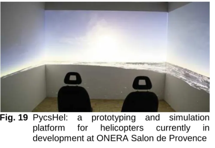
The next steps could be to use PycsHel (Fig. 19), a prototyping and simulation platform for helicopters, currently in development at ONERA Salon de Provence. Indeed, thanks to this platform, technologies such as control laws and associated operational logics can be implemented and tested easily. The gains of these control laws can be tuned using the methodology exposed in this paper. Once this is done, the gains can be implemented in the models (last step of Fig. 11) and they could be tested by pilots to evaluate the overall Handling Qualities of the aircraft with the specific gains designed.

Fig. 19 PycsHel: a prototyping and simulation platform for helicopters currently in development at ONERA Salon de Provence

6. COPYRIGHT STATEMENT

The author(s) confirm that they, and/or their company or organisation hold copyright on all of the original material included in this paper. The authors also confirm that they have obtained permission, from the copyright holder of any third party material included in this paper, to publish it as part of their paper. The author(s) confirm that they give permission, or have obtained permission from the copyright holder of this paper, for the publication and distribution of this paper as part of the ERF2014 proceedings or as individual offprints from the proceedings and for inclusion in a freely accessible web-based repository.

This work has been done thanks to funds from ONERA and Conseil Régional Provence Alpes Côte d’Azur (Pôle Pégase).

7. REFERENCES

[1] G. E. Cooper and P. Harper and G. O. Young. The Use of Pilot Rating in the Evaluation of Aircraft Handling Qualities. Appendix A. NASA TN D-5153. April 1969.

[2] B.J. Baskett and Dr. L.O. Daniel. Aeronautical Design Standard performance specification Handling Qualities requirements for military rotorcraft. United States Army Aviation and Missile Command. 2000.

[3] D. Alazard and C. Cumer and P. Apkarian and M. Gauvrit and G. Ferreres. Robustesse et Commande Optimale. CÉPADUÈS ÉDITIONS, 2000.

[4] M.B. Tischler and J.D. Colbourne and M.R. Morel and D.J. Biezad and W.S. Levine and V.

Moldoveanu. CONDUIT – A New

Multidisciplinary Integration Environment for Flight Control Development. NASA. 1997. [5] A. Luzi. Méthodologie de commande orientée

spécifications pour hélicoptères. ONERA, M2R 1/17166 DCSD. 2010.

[6] A. Badatcheff. Définition de lois de commande pour hélicoptères orientées spécification. ONERA, PFE 1/18895 DCSD. 2011.

[7] G.D. Padfield. Helicopter Flight Dynamics: The Theory and Application of Flying Qualities and Simulation Modelling, Second Edition. Oxford:Blackwell. 2007.

[8] A.R.S. Bramwell. Helicopter dynamics. AIAA. 2001.

[9] B. Benoit and A.-M. Dequin and K. Kampa and W. Gunhagen and P.-M. Basset and B. Gimonet. HOST, a general helicopter simulation tool for Germany and France. 56th Annual Forum of the American Helicopter Society. 2000.

[10] J.C. Antonioli and A. Taghizad and T. Rakotomamonjy and M. Ouladsine. Helicopter flight control design tool integrating Handling Qualities requirements. European Conference for Aerospace Sciences EUCASS. 2013. “Best student paper of the category Flight Dynamics & GNC”.

[11] J-M. Biannic. Limit-Cycles Prevention Via Multiple Hinfinity Constraints with an Application to Anti-Windup Design. In the proceedings of the 9th IFAC Symposium on Nonlinear Control Systems. Toulouse. France. 2013.

[12] C. E. Ugalde-Loo and E. Licéaga-Castro and J. Licéaga-Castro. 2x2 Individual Channel Design MATLAB® Toolbox, 44th IEEE Conference on Decision and Control, and the European Control Conference 2005.