HAL Id: hal-02456153
https://hal.archives-ouvertes.fr/hal-02456153
Submitted on 27 Jan 2020
HAL is a multi-disciplinary open access
archive for the deposit and dissemination of
sci-entific research documents, whether they are
pub-lished or not. The documents may come from
teaching and research institutions in France or
abroad, or from public or private research centers.
L’archive ouverte pluridisciplinaire HAL, est
destinée au dépôt et à la diffusion de documents
scientifiques de niveau recherche, publiés ou non,
émanant des établissements d’enseignement et de
recherche français ou étrangers, des laboratoires
publics ou privés.
Filtering out time-frequency areas using Gabor
multipliers
Ama Marina Krémé, Valentin Emiya, Caroline Chaux, Bruno Torresani
To cite this version:
Ama Marina Krémé, Valentin Emiya, Caroline Chaux, Bruno Torresani. Filtering out time-frequency
areas using Gabor multipliers. ICASSP: 45th International Conference on Acoustics, Speech, and
Signal Processing, May 2020, Barcelone, Spain. �hal-02456153�
FILTERING OUT TIME-FREQUENCY AREAS USING GABOR MULTIPLIERS
A. Marina Kr´em´e
1,2, Valentin Emiya
2, Caroline Chaux
1and Bruno Torr´esani
11
Aix Marseille Univ, CNRS, Centrale Marseille, I2M, Marseille, France
2Aix Marseille Univ, Universit´e de Toulon, CNRS, LIS, Marseille, France
ABSTRACT
We address the problem of filtering out localized time-frequency components in signals. The problem is formulated as a minimization of a suitable quadratic form, that involves a data fidelity term on the short-time Fourier transform outside the support of the undesired component, and an energy pe-nalization term inside the support. The minimization yields a linear system whose solution can be expressed in closed form using Gabor multipliers. We provide an analysis of the solu-tion and its approximasolu-tion by truncated eigenvalue expansion, and illustrate its performance on synthetic mixtures of audio signals. The proposed approach outperforms approaches that are routinely used in applications.
Index Terms— Time frequency filtering, Gabor trans-form, Gabor multipliers.
1. INTRODUCTION
Processing signals whose frequency content changes over time is widely addressed using time-frequency (TF) represen-tations [1], mainly the short-time Fourier transform (STFT) and its discrete counterpart the Gabor transform [2] for nu-merical calculations. Audio source separation is an active research field where such representations are processed [3].
A key challenge is that of filtering out localized TF com-ponents. Methods based on ridge extraction, reassignment and synchrosqueezing [4, 5, 6] model and subtract the com-ponents. One may also consider the distribution of zeros in the TF place to locate and remove components [7]. How-ever, those methods are designed to preserve the quality of the residual signal. Another strategy consists in inpainting the spectrogram coefficients related to the removed compo-nents, using nonnegative matrix factorization [8, 9] or linear interpolation with random phases [10]. The resulting spectro-grams suffer from being inconsistent [11], which often cannot be fixed by phase reconstruction methods [12].
In this paper, we investigate a non-parametric approach to filtering out a localized TF components by reconstructing a signal with STFT coefficients that both fit the original signal outside the TF support of the filtered components and by pe-nalizing the energy inside their TF support. In section 2, we propose a simple and generic formulation of the optimization
problem. The signal itself is directly reconstructed, avoid-ing any consistency issue. We show in section 3 that the so-lution is obtained in closed form. It involves the so-called Gabor multipliers [13, 14] and their spectral decomposition, which are computed independently of the hyperparameters so that they can be tuned in a computationally-efficient way. Numerical experiments proposed in section 4 reveal the de-tailed behavior of the methods, including the TF localization of the Gabor multipliers’ eigenvectors, and the quality of re-constructed target and interference sources.
2. PROBLEM STATEMENT
Let T denote a generic time-frequency transform, mapping
any x ∈ CL to T x ∈ l2(Λ), Λ being the discrete
time-frequency domain. Our goal is to filter out signal compo-nents located in a given region of the TF plane, in the
fol-lowing setting: we assume that the observed signal x0is of
the form x0 = xref + xper, i.e. the sum of a target signal
xref, and a perturbation xper. While no assumption is made
on the target signal, we assume further that the STFT of xper
is strongly concentrated in a known region Ω ⊂ Λ. We denote
by Ω = Λ\Ω the complement region. Estimating xref from
the observation x0 and from the knowledge of support Ω is
a specific denoising or source separation problem which we formulate as x∗= argmin x∈CL kT x − T x0k2Ω+ λkT xk2Ω. (1) where kyk2 Ω := P k∈Ω|y[k]|
2and λ > 0. The first term of
the objective function in (1) is a data fidelity term that en-forces the STFT of the estimated signal to fit that of the ob-servation outside Ω. The second term controls its energy in Ω, and the regularization parameter λ controls the trade-off between the two terms.
Here and throughout the paper, we will focus on the Ga-bor transform although problem (1) can be solved in a more general case. We first introduce some definitions and nota-tions. Let a and b denote the time and frequency sampling period, assumed to be divisors of L, and set N = L/a, M = L/b. N and M are respectively the numbers of time shifts and frequency shifts. The TF domain is the lattice
Λ = ZM × ZN. For a window function g ∈ RL, the
Gabor atom gmn at TF point (m, n) ∈ Λ is defined by
gmn[l] = g(l − na)e2iπmbl/M, ∀l ∈ ZL. The Gabor
trans-form Vgx ∈ CM ×N of x is defined by Vgx[m, n] = hx, gmni = L−1 X l=0 x[l]g[l − na]e−2iπmbl/M.
Given the adjoint Vg∗of Vg, also called synthesis operator,
the frame operator S = Vg∗Vg is bounded, self-adjoint and
semi-positive definite. If S > 0, S is invertible, which
per-mits to reconstruct any x ∈ CL from its Gabor coefficients.
Of particular interest are the so-called Parseval frames, for
which S = I, i.e., Vg∗is a left inverse of Vg. For the sake of
simplicity, we focus on this case in this paper.
3. ANALYTICAL RESOLUTION
Using Gabor multipliers introduced in section 3.1, the analyt-ical solution of problem (1) is established in section 3.2.
3.1. Gabor multipliers
Gabor multipliers are linear operators on CL defined by
pointwise multiplication with a TF transfer function called a Gabor mask, in the Gabor coefficients domain. Denoting by m the Gabor mask, we will also denote for simplicity by m the operator of pointwise multiplication by m.
Definition 3.1 The Gabor multiplier associated to (g, Λ)
with maskm is defined by Mm= Vg∗mVg, i.e.,
Mmx =
X
m,n
m[m, n]hx, gm,nigm,n.
Gabor multipliers have been studied extensively (see [15, 16] and references therein). We recall below some important properties that will be of interest in the sequel.
Properties 3.1
(i) Ifm is real-valued then Mmis self-adjoint. Then there
is an orthonormal basis of CL formed by Mm
eigen-vectors.
(ii) The Gabor multiplier generated bym ≡ 1 is a multiple
of the identity operator if and only if(g, Λ) generates a
tight Gabor frame.
(iii) Ifm ∈ CM ×N, then Mm defines a bounded operator
with operator normkMmkop≤ Ckmk∞, whereC is a
constant. In particular, ifg and Λ generate a Parseval
frame, thenkMmkop≤ kmk∞.
3.2. Analytical solution
Let f (x) = kVgx − Vgx0k2Ω+ λkVgxk2Ω be the objective
function in (1) for T = Vg. f is a quadratic form and
there-fore its minimization results in a linear system. For simplicity,
we denote by MΩand MΩthe multipliers associated with the
indicator functions1Ω and1Ω considered as Gabor masks.
We obtain
5f (x) = 2(MΩ+ λMΩ)x − 2MΩx0.
Since Vg∗Vg = I, we have MΩ = I − MΩand then MΩ¯ +
λMΩ = [I + (λ − 1)MΩ]. According to property 3.1 (iii) ,
(MΩ+ λMΩ) is invertible if 0 < λ < 2. Then:
5f (x∗) = 0 ⇐⇒ x∗λ= (MΩ+ λMΩ)−1MΩx0.
As the mask is real valued and using properties 3.1(i) and 3.1(iii), there is an unitary matrix U and a diagonal matrix
D = diag(σ1, ..., σL), σ1 ≥ · · · ≥ σL such that MΩ =
U DU−1. Setting γl= 1−(1−λ)σλσl l, we then have:
x∗λ= x0− U diag (γ1, . . . , γL) U−1x0. (2)
While the above L × L matrices can be very large, the Gabor multipliers under consideration act on much lower
di-mensional subspaces. The eigenvalues σlbeing sorted in
de-creasing order, sequence {γl, l = 1, · · · L} is decreasing too,
which can be used for truncation purpose. Let be x∗K be the
solution obtained when only the K < L largest eigenvalues
are retained, i.e. x∗K = U1:Kdiag (γ1:K) U1:K−1x0. The
trun-cation error is controled by
kx∗λ− x∗Kk = k diag(0, · · · 0, γK+1, · · · , γL)U−1x0kCL
≤ γK+1kU−1x0kCL ≤ γK+1kx0k (3)
4. EXPERIMENTS
We illustrate the approach on a synthetic mixture of two real audio signals. We first describe the signals, before analyzing the action of Gabor multipliers and discussing results. 4.1. Experimental setting
The sounds were provided by ANSYS VRXPERIENCE
Sound Analysis and Specification1. The target signal x
ref
is a car engine sound and the perturbation signal xper is a
birdsong. Both signals have been sampled at fs = 8000 Hz and are L = 8192 samples long. The Gabor transform for each of these signals is calculated with a Hann window of length 128, the time-frequency lattice parameters are set to a = 32 and b = 512, generating a 256 × 256 TF matrix. The observation is a linear combinations of these two signals, as shown in Fig. 1. The spectrograms of the engine sound and birdsong are displayed in the first row of Fig. 4.
The goal is to filter out the birdsong. To this end, a mask m was constructed as the indicator function of a region Ω matching the six high frequency components as shown in Fig. 1. The mask is constructed from spectrograms of both sources as:
mij =
(
1 if |Vgxper(i, j)| < 2|Vgxref(i, j)|.
0 else 0 2000 4000 6000 8000 Time (samples) 0 0.2 0.4 0.6 0.8 1 Frequency (normalized) -80 -60 -40 -20 0 0 2000 4000 6000 8000 Time (samples) 0 0.2 0.4 0.6 0.8 1 Frequency (normalized) -80 -60 -40 -20 0
Fig. 1. Sum of an engine’s sound and a birdsong: observa-tions (left) and binary mask (right).
The closed-form solution (2) depends on the regulariza-tion parameter 0 < λ < 2, which is adjusted using the fol-lowing strategy. We choose the optimal λ as the value for
which the energy of the reconstructed signal kVgx∗λk2Ωwithin
the region Ω matches the energy E = kVgx0k2Ω0 in another
region Ω0similar to and disjoint from Ω. Ω0is grossly chosen
by hand here and this process may be automated if needed. Such tuning of λ is computationally efficient: since the spec-tral decomposition of the Gabor multiplier does not depend on λ, testing each value of λ mainly requires the truncated
matrix-vector multiplications to build x∗K and the
computa-tion of its Gabor transform.
4.2. Gabor multiplier’s spectral decomposition
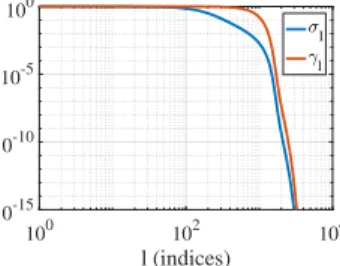
The Gabor multiplier eigenvalues σl and coefficients γl are
shown in Fig. 2. Only the first 4000, which are above
nu-merical accuracy, are displayed. γ values below 10−5 were
truncated, leading to a K = 1 696-dimensional subspace.
100 102 104 l (indices) 10-15 10-10 10-5 100 l l
Fig. 2. Gabor multiplier’s eigenvalues σland coefficients γl.
Interestingly, the spectral decomposition of the Gabor
multiplier MΩtends to separate contributions from the
vari-ous connected components. For example, we display in Fig. 3
the spectrograms of the 100th and 1500th eigenvectors, to-gether with the time and spectral representations. The first one appears to be sharply localized in the region of one of the component, while the other one is closer to its bound-ary. This is in agreement with the usual behavior of Gabor multiplier eigenfunctions. However we find quite interesting the fact that multipliers associated with disconnected regions tend to generate eigenfunctions localized in the connected components. -4000 -200 0 0.2 0.4 0.6 0.8 1 Normalized frequency 0 2000 4000 6000 8000 -0.2 0 0.2 0 2000 4000 6000 8000 Time (samples) 0 0.2 0.4 0.6 0.8 1 -200 -100 0 0 0.2 0.4 0.6 0.8 1 Normalized Frequency 0 2000 4000 6000 8000 -0.1 0 0.1 0 2000 4000 6000 8000 Time (samples) 0 0.2 0.4 0.6 0.8 1
Fig. 3. Waveform, spectrogram and spectrum of the 100th (left) and 1500th (right) eigenvectors of the Gabor multiplier.
4.3. Comparative reconstruction results
We compare here results obtained with the proposed
ap-proach, hereafter termed RedEnerg, with results obtained
using two approaches commonly used in industrial applica-tions:
• ZerVal(zero values): set to zero coefficients within the
region Ω before inverting the Gabor transform, i.e.
ap-ply the Gabor multiplier MΩ.
• RandVal(random values, as implemented in the
com-mercial software SAS [10]): estimate the Gabor coef-ficient modulus within Ω by linear interpolation along the frequency axis, then turn to complex coefficients by generating random, uniformly distributed phases, be-fore inverting the Gabor transform.
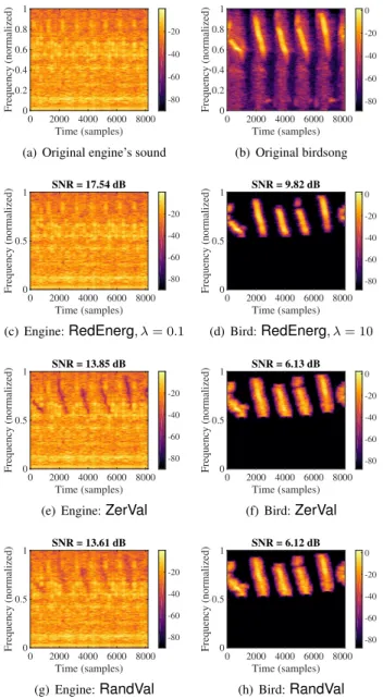
The spectrograms of the target signal and the
perturba-tion signal reconstructed byRedEnerg,ZerValandRandVal
respectively are presented in Fig. 4. Regarding the engine
sound (left column), the spectrogram of theRedEnerg
recon-struction (Fig. 4, 2nd row) is visually very close to the orig-inal, while significant differences can be seen with the
out-puts ofZerValandRandVal(respectively 3d and 4th rows of
Fig. 4), where the birdsong is still present. Regarding the
bird-song (right column), RedEnerg also outperforms the other
two methods. Note that the birdsong reconstructions are of poorer quality because the low frequency part of the chirps was not included in the domain Ω.
Quantitative assessment of reconstruction quality for xref
values are displayed at the top of spectrograms in Fig. 4. The evolution of SNR as a function of λ is displayed in
Fig 5, together with SNR values obtained withZerVal and
RandVal. The plot shows that the SNR value for the optimal
λ value is significantly better than those obtained byZerVal
andRandVal, which confirms the visual impression.
0 2000 4000 6000 8000 Time (samples) 0 0.2 0.4 0.6 0.8 1 Frequency (normalized) -80 -60 -40 -20
(a) Original engine’s sound
0 2000 4000 6000 8000 Time (samples) 0 0.2 0.4 0.6 0.8 1 Frequency (normalized) -80 -60 -40 -20 0 (b) Original birdsong SNR = 17.54 dB 0 2000 4000 6000 8000 Time (samples) 0 0.5 1 Frequency (normalized) -80 -60 -40 -20 (c) Engine:RedEnerg, λ = 0.1 SNR = 9.82 dB 0 2000 4000 6000 8000 Time (samples) 0 0.5 1 Frequency (normalized) -80 -60 -40 -20 0 (d) Bird:RedEnerg, λ = 10 SNR = 13.85 dB 0 2000 4000 6000 8000 Time (samples) 0 0.5 1 Frequency (normalized) -80 -60 -40 -20
(e) Engine:ZerVal
SNR = 6.13 dB 0 2000 4000 6000 8000 Time (samples) 0 0.5 1 Frequency (normalized) -80 -60 -40 -20 0 (f) Bird:ZerVal SNR = 13.61 dB 0 2000 4000 6000 8000 Time (samples) 0 0.5 1 Frequency (normalized) -80 -60 -40 -20 (g) Engine:RandVal SNR = 6.12 dB 0 2000 4000 6000 8000 Time (samples) 0 0.5 1 Frequency (normalized) -80 -60 -40 -20 0 (h) Bird:RandVal
Fig. 4. Spectrogram of the reconstructed signals. Left col-umn: Engine’s sound. Right colcol-umn: Birdsong.
The performance assessment of the proposed method is confirmed when extending the same experiments to other
sounds, downloaded from Freesound2. Target sounds include
a car engine, a train and an airplane while 4 pertubation sig-nals well located in the TF plane are used: some beeps, a finger snap, clicks and another birdsong. For each mixture,
2https://freesound.org 10-10 100 1010 (values) 5 10 15 20 25 SNR (dB) RedEnerg ZerVal RandVal (a) Target 10-10 100 1010 (values) -5 0 5 10 15 SNR (dB) RedEnerg ZerVal RandVal (b) Perturbation
Fig. 5. SNR in decibels (dB) for the three solvers. the SNRs calculated between engine sound and the signal estimated by the three solvers are summarized in Table. 1 and show the superiority of the proposed method.
From a computational viewpoint, all methods were imple-mented in MATLAB on a macOS system with 2.3 GHz Intel core i5. The most time-consuming part is the diagonaliza-tion of the multiplier (about 306 seconds), which is done only once. The computation of the solution then being very fast: the adjustment of the regularization parameter λ, that involves many evaluations of the solution, took about 114 seconds.
car train aircraft
RedEnerg 25.05 23.88 26.80 Beeps ZerVal 24.23 16.52 24.73 RandVal 24.90 16.15 24.73 RedEnerg 18.88 22.49 20.72 Finger snap ZerVal 17.18 20.70 16.59 RandVal 16.92 16.17 15.93 RedEnerg 21.67 20.97 17.96 Clicks ZerVal 17.61 13.98 12.33 RandVal 10.57 5.60 11.07 RedEnerg 18.01 21.52 20.04 Birdsong ZerVal 17.4 21.52 19.71 RandVal 17.13 21.28 19.56
Table 1. SNRs for several targets and perturbations. 5. CONCLUSION
We have addressed the problem of estimating a target signal, with no assumption on its contents, when perturbated by an additive signal that is well located in an region Ω of the TF plane. We have proposed an optimization problem in which the energy in Ω is controlled. It admits an analytical solution, which provides the estimated signal directly, without suffer-ing from TF consistency issues. The underlysuffer-ing Gabor mul-tipliers eigenvectors show interesting localization properties and the proposed method outperforms some industrial base-line systems in terms of reconstruction SNR. Future direc-tions may include the problem formulation with other penalty terms in order to provide alternate ways to control the con-tents of the masked TF regions.
6. REFERENCES
[1] K. Gr¨ochening, Foundations of Time-Frequency Analy-sis, Birkh¨auser, Boston (MA), 2011.
[2] D. Gabor, “Theory of communication. part 1: The anal-ysis of information,” Journal of the Institution of Elec-trical Engineers - Part III: Radio and Communication Engineering, vol. 93, no. 26, pp. 429–441, Nov. 1946. [3] E. Cano, D. FitzGerald, A. Liutkus, M. D. Plumbley,
and F.-R. Stoter, “Musical source separation: An intro-duction,” IEEE Signal Processing Magazine, vol. 36, no. 1, pp. 31–40, Jan. 2019.
[4] F. Auger, P. Flandrin, Y.-T. Lin, S. Mclaughlin, S. Meignen, T. Oberlin, and H.-T. Wu, “Time-frequency
reassignment and synchrosqueezing: An overview,”
IEEE Signal Process. Mag., vol. 30, no. 6, pp. 32–41, 2013.
[5] I. Daubechies, J. Lu, and H.-T. Wu, “Synchrosqueezed wavelet transforms: An empirical mode decomposition-like tool.,” Appl. and Comp. Harm. Anal., vol. 30, no. 1, pp. 243–261, 2011.
[6] G. Thakur and H.-T Wu, “Synchrosqueezing-based
recovery of instantaneous frequency from nonuniform samples,” SIAM J. Math. Anal, vol. 43, pp. 2078–2095, 2011.
[7] P. Flandrin, “Time-frequency filtering based on spectro-gram zeros,” arxiv.org, 2015.
[8] J. Le Roux, H. Kameoka, N. Onoa, A. de Cheveign´e, and S. Sagayama, Computational auditory induction as a missing-data model-fitting problem with Bregman di-vergence, vol. 53, Speech Communication, May-June 2011.
[9] P. Smaragdis, B. Raj, and M. Shashanka, “Missing data imputation for spectral audio signals,” IEEE Int. Work-shop Mach. Learn. Signal Process., 2009.
[10] ANSYS VRXPERIENCE, “Sound website,”
https://www.ansys.com/fr-fr/products/systems/ansys-vrxperience/sound.
[11] J. Le Roux and E. Vincent, “Consistent Wiener filtering for audio source separation,” IEEE Signal Process. Lett., vol. 20, no. 3, pp. 217–220, Mar. 2013.
[12] Z. Prusa, P. Balazs, and P. Sondergaard, “A non-iterative method for reconstruction of phase from STFT magni-tude,” in IEEE/ACM Trans. Audio Speech Lang. Pro-cess., 2017, vol. 25, pp. 1154–1164.
[13] P. Depalle, R. Krondland-Martinet, and B. Torr´esani, “Time-frequency multipliers for sound synthesis,” Proc. SPIE, vol. 6701, 2007.
[14] M. D¨orfler and B. Torr´esani, “On the time-frequency representation of operators and generalized gabor mul-tiplier approximations,” Journal of Fourier Analysis and Applications, vol. 16, pp. 261–293, 2010.
[15] M. D¨orfler, Gabor analysis adapted to music, Ph.D. thesis, University of Vienna, Austria, 2002.
[16] H. G. Feichtinger and K. Nowak, A first survey of Gabor multipliers, Advances in Gabor Analysis, 2002.