From Workflow Models to Document Types and Back Again

RESEARCH OUTPUTS / RÉSULTATS DE RECHERCHE

Author(s) - Auteur(s) :

Publication date - Date de publication :

Permanent link - Permalien :

Rights / License - Licence de droit d’auteur :

Institutional Repository - Research Portal

Dépôt Institutionnel - Portail de la Recherche

researchportal.unamur.be

University of Namur

From Workflow Models to Document Types and Back Again

van Hee, Kees; Hidders, Jan; Houben, Geert-Jan; Paredaens, Jan; Thiran, Philippe

Publication date:

2007

Document Version

Early version, also known as pre-print

Link to publication

Citation for pulished version (HARVARD):

van Hee, K, Hidders, J, Houben, G-J, Paredaens, J & Thiran, P 2007, From Workflow Models to Document

Types and Back Again. Technische Universiteit Eindhoven, Eindhoven.

General rights

Copyright and moral rights for the publications made accessible in the public portal are retained by the authors and/or other copyright owners and it is a condition of accessing publications that users recognise and abide by the legal requirements associated with these rights. • Users may download and print one copy of any publication from the public portal for the purpose of private study or research. • You may not further distribute the material or use it for any profit-making activity or commercial gain

• You may freely distribute the URL identifying the publication in the public portal ? Take down policy

If you believe that this document breaches copyright please contact us providing details, and we will remove access to the work immediately and investigate your claim.

From Workflow Models to Document Types and Back Again

Kees van Hee

Jan Hidders

Geert-Jan Houben

Jan Paredaens

Philippe Thiran

Abstract

The best practice in information system development is to model the business processes that have to be supported and the database of the information system separately. This is inefficient because they are closely related. Therefore we present a framework in which it is possible to derive one from the other. To this end we introduce a special class of Petri nets, called Jackson nets, to model the business processes, and a document type, called Jackson types, to model the database. We show that there is a one-to-one correspondence between Jackson nets and Jackson types. We illustrate the use of the framework by an example.

Contents

1 Introduction 3

2 Context and motivation 3

2.1 Historical perspective . . . 3 2.2 The relationship between workflow and document management . . . 5 2.3 Example: Patient Care System . . . 5

3 Jackson Types 7

4 Jackson Nets 11

4.1 Petri nets and workflow nets . . . 11 4.2 Jackson nets and soundness . . . 13

5 The Jackson Types of Jackson Nets 17

5.1 The variety in Jackson nets generated by a certain Jackson types . . . 17 5.2 The variety in Jackson types from which a certain Jackson net is generated . . . 18 5.3 Characterizing the expressive power of Jackson Nets . . . 23

6 Case Study 27

7 Related work 30

8 Conclusion 32

1

Introduction

Data modeling and process modeling are two essential activities in requirements analysis and design of information systems. They are using different techniques and normally they are per-formed independently. Since both techniques are defining essential aspects of an information system they have to be integrated at some point in the development process, but normally this is at the level of programming. In this paper we show that data modeling and process model-ing can go hand in hand from the beginnmodel-ing of the development process of so-called case-based information systems. The characteristic of these information systems is that they are developed to support the handling of cases, such as the treatment of a patient, the handling of an order or the delivery of a service. For each case type there is a workflow defining the tasks to be performed for the case. A workflow is a process with a clearly defined start and end state. In this paper we use a special class of Petri nets to model workflows, the so-called workflow nets [20]. Since in each task of the workflow something happens to the case, it is to be expected that the data type to record the case data is related to the structure of the workflow. The case data is recorded in the case document, the structure of which is a document type. We show that if we restrict ourselves to a special class of workflow nets, the so-called Jackson nets, then there is a tree shaped document type for the case data, called the Jackson type, that contains the same information as the workflow net. One of the main results in this paper is that there is a one-to-one correspondence between the document type and the workflow description, so from one we can derive the other. This is similar to the classical program design method of Jackson [6] which is the reason we called the workflow nets and the document types after this author.

The organization of the rest of this paper is as follows. In Section 2 we give the system development context for our work and we give a motivating example. In Section 3 we introduce Jackson types. In Section 4 we introduce the Jackson nets and in Section 5 we study the relationships between Jackson nets and Jackson types. In particular we prove that if two Jackson nets are derived from the same Jackson type they are isomorphic and that if it is possible to derive the same Jackson net from two different Jackson types, these types are algebraical equivalent. In Section 6 we continue with the motivating example. Here we show how we can derive an XML document type from a Jackson net and demonstrate how it provides a logical structure that helps the user to formulate queries over the cases of the workflow. Finally, we discuss related work in Section 7. The conclusion of the paper is given in Section 8.

2

Context and motivation

2.1

Historical perspective

In the requirements analysis and design phases of an information system we describe the desired functionality of a system from different perspectives. In the early stages of systems design, say until 1970, the systems designers started to describe the processes the system had to fulfil in terms of flowcharts. Since flowcharts describe only sequential processes (one thread of control) the interactions between processes was left out.

In the eighties the data modeling techniques became popular. Versions of the entity relation-ship model or the relational model were used for this. The big advantage of using this so-called database-oriented approach was that after the types of the data stores where established by a data model, several designers could model concurrently the processes that would act on the data stores . The modeling of the operations, i.e. of transformations on data objects, was done again at the low level of flowcharts or directly in a programming language.

model the data aspect and the operations on the data in an integrated way. However the processes of a system were still second class citizens. Therefore process-aware information systems were identified as special class of systems [4]. This went so far that special software components were designed for the coordination of many interacting processes. Terms as “workflow management”, “orchestration” and “choreography” are used to refer to this functionality. Special coordination engines were developed, for instance workflow management systems.

Modeling languages for the process appeared. They are also used to configure the coordination engines, like the database schema is a configuration parameter of a database management system. There are two families of formal languages for modeling processes: process algebra’s and Petri-nets. Besides these there are several industry standards for modeling processes, such as BPEL (business process execution language), UML activity diagrams, and BPMN (business process modeling notation). These languages allow us to design the process aspect of a system in isolation. These process modeling languages allow concurrency and so the problems of the days of the flowcharts were overcome.

The problem that we address is the integration of the different views: the data view and the process view. Already in the seventies there was a successful attempt to design the data and process aspect in an integrated way, JSP, Jackson’s programming method [6] and later the method was lifted to the level of system design, JSD, Jackson’s development method [7]. (In Software requirements and specifications [8] an overview is presented.) In this approach hierar-chical program structures where derived from the hierarhierar-chical input and output data structures, but they became out of fashion when the relational data model appeared. More recently UML also allows the specification of links between the process models and data models, but these models are here only loosely coupled and they remain essentially independent.

The programming method JSP was based on the idea that programs transform data streams into data streams. A data stream was a sequence of data elements and these data streams had a hierarchical data type. In fact, the data types of the input and output streams had to be describable by regular expressions composed of three kinds of operators: sequential composition, selection and iteration. The input and output data types were represented as so called tree diagrams and they were combined into one tree that represented the program structure. In fact, the program structure was also a tree diagram and the input tree and the output tree could be derived from the program tree by projections. The central idea of JSP was that the data structures determine the program structure. So JSP started with designing the input and output data structures. This idea is in line with the database oriented approach although in JSP hierarchical data structures are essential instead of the relational structure.

The similarity between the Jackson data structures and regular expressions was a reason to compare JSD, the development method based on JSP, with the language for communicating sequential processes, CSP, which can describe regular expressions as well. Therefore Sridhar and Hoare expressed JSD in CSP [19]. To our knowledge this was the first attempt to relate Jackson data structures and process structures in a fundamental way, but there was not much follow up from this attempt.

Another approach to formally integrate processes and data are colored Petri nets where tokens have values that may be changed by transitions [9]. The values are represented as colors and these colors can be linked to edges to indicate that only tokens with a certain color are consumed or produced through them. However, this approach does not offer a way to integrate the types of these colors into a global data model for the process as a whole.

The best practice today in information system development is to model the business processes that have to be supported and the database of the information system separately. This seems to be inefficient because they are often closely related. Like the observations of Jackson, we should try to exploit this relationship as much as possible.

2.2

The relationship between workflow and document management

Today there is a revival of hierarchical data structures as illustrated by the popularity of the many XML-based standards. There are several reasons for this. One is that hierarchical structures occur frequently in practice. For instance the bill of material of a physical artefact like bicycle or an airplane is a hierarchical structure. In the service industry we encounter also many hierarchical data structures, consider for instance the electronic patient record in health care, a bill of lading for a complex transport or the insurance portfolio of a company. In fact they all are described by a document and documents have hierarchical structures, composed with the operators: sequence, selection and iteration. In relational databases these documents are refined into their constituting elements and these are distributed over many tables. As soon as a document is needed the elements are retrieved from the tables and presented as a whole to the user who can update this view and restore it. From an implementation point of view this might be efficient, but from a conceptual point of view it is more natural to consider a document as one, structured, entity. The relational view is only interesting if management information is considered where a survey over different documents is needed.

Because documents are a natural concept for modeling data in business processes that pro-duce physical artifacts or services, generic software components were developed to take care of documents, the document management systems. There is a natural relationship with workflow management systems, since both type of components are supporting (primary) business pro-cesses. In business process management [23] the processes and the data are equally important. The linking pin is what is called the case. A case is an instance of a case type and it is the “thing” that is moving through the business process. For instance in a bicycle factory the case is the construction of the bicycle from the order form till the final product. In a service organization like a hospital the case is the treatment of a patient, starting with its first visit till his final one (see Section 6).

There is often a case document that records everything that happened to the case, so the state of the process can be reconstructed from the case document and vice versa. This is not always necessarily the situation at the level of processes and document types, i.e., the document type does not contain a complete process description. There is however often a close relationship, e.g., the bill of material of a bicycle has a structure that reflects the construction process of the bicycle [17]. In this paper we define and study a class of models for which there is such a one-to-one relationship between document types and processes, namely the Jackson types and Jackson nets which are introduced in Section 3 and Section 4.

2.3

Example: Patient Care System

There are many Electronic Patient Record (EPR) systems that are used to record and plan the medical events in the treatment of a patient. The focus of these systems is in registration of observations and decisions. Today medical protocols play an important role in the patient care processes. The protocols describe a care process that can be seen as the best practice. Medical experts have protocols for deriving a diagnosis as well as for a treatment. The traditional EPR systems are database-oriented and have little support for process control. In the Patient Care systems of the future the process control aspect will become more important and therefore the process knowledge should be integrated with the patient data. In fact a Patient Care system is a very good example of a case handling system, where we may consider the treatment of each medical problem as a different case. An alternative, that we do consider here is to view the whole life of a patient as one case.

As an illustration we consider a simplified care process of patient care in a hospital. The process is expressed as a Petri net in Figure 1. A formal definition of a (labeled) Petri net is

given in Section 4.1. A Petri net is a bipartite graph with nodes of type place and nodes of type transition. A place indicates a possible stage or phase in the care process. A place may be marked with a token, which is in our situation a reference to the patient. A transition models an event, activity or task in the care process, and the label of the transition indicates the type of event. The case is here the patient. The set of all tokens belonging to one patient indicates the state of the patient. Note that a patient can be in different stages at the same time. So the stages a patient is in at some moment form its state.

Some transitions are only needed to describe the control flow and have no real task associated to it. This is the case with task 11: “Double test” and task 14: “End double test”. Next we describe the meaning of the process model.

A patient who enters the hospital first goes to the reception desk (task 1: Patient identi-fication). If the patient comes to the hospital for the first time, the patient’s personal data is registered (task 3: New patient). This data consists of the patient’s name and address (street, zip code and city) and a reference to its general physician. In case the patient is known to the hospital only an identity card is requested and the relevant personal data is fetched from the database (task 2: Known patient). Then the patient’s problem is registered (task 4: Problem registration), a doctor is selected for a first examination and the patient receives an admission ticket that contains a number, the date and time of the admission.

After the patient has explained its problem, a preliminary diagnosis is made (task 5: Prelim-inary diagnosis).

Depending on the outcome of this diagnosis, either Test 1, or Test 2, or both Test 1 and Test 2 in parallel, or both Test 1 and Test 2 in any order, or some treatment protocol is chosen from Protocols 1, 2 and 3. It may occur that no treatment is possible or needed, in which case the patient leaves the hospital and some administration is performed (task 16: Exit). Examples of tests are laboratory tests like urine or blood tests and image generation like X-ray or a MRI-scan. Today there are many protocols for medical treatment. Protocols may consist of tests as well as therapies and may be refined to sub-processes.

All tests result in data of the same type: the type of result (chosen from the official list of activity types from the hospital), the date, and the resulting values (outcomes) of the analysis.

After the tests or protocols have been executed they are evaluated in a new diagnosis (task 15: Diagnosis). Depending on the outcome of this diagnosis, a selection of further activities is made. This is repeated until the decision is made that further treatment is not useful anymore. There is for each patient (case) a dossier which is the EPR. Two typical instances are dis-played in Figure 2. The dots represent data entered by the medical experts, and may include observations, decisions or any data involved in the event. The first dossier starts with the in-formation for identifying the patient, the registration of the new patient, the registration of the problem and the result of the preliminary diagnosis. Then there is a list of treatments and finally the registration of the exit of the patient. The list of treatments consists here of three treatments all ending with a diagnosis. In the final treatment we see that the double test is applied and so the information involved in preparing the two tests, the two tests themselves and the combination of the test results is stored. In the second dossier we see largely the same type of information except that here the patient is registered as a known patient and the list of treatments consists of the double test followed by the protocol3 test. It is not hard to see how the data structure of such dossiers can often be described by a type consisting of recursively nested records and lists. Observe that the relative vertical and horizontal orientation of the steps in the dossiers has meaning here: a step that is just below another step describes an event that followed the event of the step just above it, and steps that are next to each other describe events that were executed in parallel. This relationship between the parts of the dossier may determine how the dossier is allowed to grow. For example, the information for “preliminary diagnosis” may not be

pi pi a _{1: Patient} identification b 2: Known patient 3: New Patient c _{4: Problem} registration d 5: Preliminary diagnosis _e 15: Diagnosis 16: Exit po k 12: Test 2 11: Double test 9: Test 1 8: Protocol 3 6: Protocol 1 7: Protocol 2 10: Test 1 13: Test 2 14: End double test f g h i j

Figure 1: A workflow for handling a medical problem

entered before the information for “problem registration” is entered, but for the double test the information for “test2” may be entered before that of “test1”. Therefore we extend the notion of type such that it also captures these relationships and we investigate the precise relationship between such types as a workflow description formalism and certain workflow nets.

In the presented example the different pieces of information are associated with the firing of transitions, i.e., each firing of a transition generates some information that is to be stored in the patient dossier. It can however in some cases be more natural to think of the information as being associated with the tokens, for example if the token represents a document containing a diagnosis or a form that contains the result of a test. Therefore we assume in the following of the paper that information can be associated both with the firing of a transition and with the tokens that are consumed and produced.

3

Jackson Types

In this section we introduce types that we use to represent workflow document types, i.e., data structures that can contain all the information that is involved in a single case of the workflow that is described by a workflow net. We show that these types (1) can indeed contain all the involved information and (2) have a natural correspondence to the hierarchical structure of the workflow net.

patient identification: ... new patient: ... problem registration: ... preliminary diagnosis: ... treatments: test1: ... diagnosis: ... protocol2: ... diagnosis: ... double test: ... test pair: test1: ... test2: ... end double test: ... diagnosis: ... exit: ... patient identification: ... known patient: ... problem registration: ... preliminary diagnosis: ... treatments: double test: ... test pair: test1: ... test2: ... end double test: ... diagnosis: ... protocol3: ... diagnosis: ... exit: ...

Figure 2: Examples of two patient dossiers

all the information involved in a certain transition or place of a workflow net. Note that these atomic types are only atomic for the purpose of describing the workflow document type and may in a later phase of the modeling process be broken down into smaller components. From these atomic types we construct types by using constructors for sequencing (;), parallelism (k), choice (+), and loop (#).

Definition 3.1 (Type). The set of types J is defined by the following syntax:

J ::= A | (J ; J ) | (J k J ) | (J + J ) | (J # J ).

The types can be thought of as a combination of a data type and a process specification. The type (τ1; τ2) denotes the type of ordered records. This type describes records with fields of

type τ1 and τ2 and indicates that in the process the event associated with the field of type τ1

precedes the event associated with the field of type τ2. The type (τ1 k τ2) denotes the type of

unordered records with fields of type τ1 and τ2that describes records with fields of type τ1 and

τ2 and indicates that in the proces there is no particular order. The type (τ1+ τ2) denotes the

type of variant records that contain either a value of type τ1 or τ2. Finally the type (τ1#τ2)

denotes nonempty lists of values of type τ1 separated by values of type τ2.

The notion of trace set is introduced to formalize the concept of all information that is involved in a single run of a workflow. Here a single trace is a string of atomic types and a trace set is a set of such strings. If α and β are such strings then we will denote the concatenation of α and β as α · β.

The trace set that is associated with a certain type is defined as follows.

Definition 3.2 (Trace-set of Types). The trace-set of a type τ , T r(τ ) is defined by induction upon the structure of τ as follows:

• T r(τ ) = {τ } if τ ∈ A

• T r((τ1; τ2)) = {α · β | α ∈ T r(τ1), β ∈ T r(τ2)}

• T r((τ1k τ2)) = {α1· β1· . . . · αk· βk| k ≥ 0, α1· . . . · αk ∈ T r(τ1), β1· . . . · βk ∈ T r(τ2)}

• T r((τ1+ τ2)) = T r(τ1) ∪ T r(τ2)

We have for example • T r(((a; b) + c)) = {ab, c}

• T r((a; (b#c))) = {ab(cb)n _{| n ≥ 0}}

• T r((b + d)) = {b, d}

• {abdcbcb, abcbb, abb} ⊂ T r((a; (b#c)) k (b + d)) )

Remark that a#b stands for (a; b)∗; a, using the Kleene-star.

Definition 3.3 (Trace Equivalence of Types). Two types τ and τ0 _{are called trace equivalent,}

denoted as τ ≡trτ0, iff T r(τ ) = T r(τ0).

Theorem 3.4. There is no finite set of equivalence rules that defines the trace equivalence of types.

Proof. Let us assume that there is such a finite set of equivalence rules. Then this set of rules will also define trace equivalence if there is only one letter in the alphabet. Under this assumption e1 k e2 ≡tr e1+ e2, so there is also such a set of rules for expressions that do not contain

k. We can express the # operator with the Kleene-plus (denoted e+_{) and vice versa, because}

e+_≡

tr(e#e) + (e; (e#e)) and e1#e2≡tre1+ (e1; (e2; e1)+). It follows that there is also such a

set of rules for the language with the Kleene-plus but without #. There is also such a set of rules if we add the empty string (denoted as ε) since we can rewrite every expression to either a ε-free e or ε + e with e ε-free by using only a finite set of equivalence rules. There will then also be such a set of rules for the language with the Kleene-plus replaced with the Kleene-star (denoted e∗) since one can be expressed with the other, and vice versa: e∗≡trε + e+ and e+≡tre; e∗. Note

that the resulting language is exactly the language of regular expressions. However, for that language it has been shown by Aceto, Fokkink and Ing´olfsd´ottir [1] that such a finite set of rules does not exist, even under the assumption that there is only one symbol in the alphabet.

Conjecture 3.5. Deciding trace inequivalence of types is EXPSPACE complete.

The problem is very similar to the problem of deciding trace inequivalence of regular expres-sions extended with interleaving operations, which was shown to be EXPSPACE complete by Mayer and Stockmeyer [12].

Next to trace equivalence we also define another coarser notion of equivalence that can be informally thought of as defining when two types represent the same data type. For example the types (a; (b; c)) and ((a; b); c) can be seen as representations of the type (a; b; c), i.e., the type of ordered tuples with the fields a, b and c in that order. Another example are (a k b) and (b k a) which both represent the type of unordered tuples with the fields a and b. This leads to the following definition.

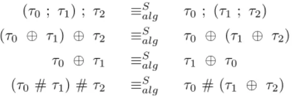
Definition 3.6 (Algebraic Equivalence of Types). The algebraic equivalence ≡algis the smallest

equivalence relation on the set of types that fulfils the identities of Figure 3.

Note that the identity between τ0 # (τ1# τ2) and (τ0# τ1) # τ2is not included since these

two types might not even be trace equivalent. For example, the trace aca is in T r(((a#b)#c)) but not int T r((a#(b#c))), and the trace abcba is in T r((a#(b#c))) but not in T r(((a#b)#c)). The definition of the notion of algebraic equivalence of types will be further motivated later on in the paper where it is shown that for a certain non-deterministic procedure that derives types for a certain class of workflow nets it captures exactly the ambiguity of this procedure, i.e., there may be more than one possible result type but they are all algebraically equivalent.

That algebraic equivalence is indeed coarser then trace equivalence is established by the following theorem.

(τ0 ; τ1) ; τ2 ≡alg τ0 ; (τ1 ; τ2) (τ0 k τ1) k τ2 ≡alg τ0 k (τ1 k τ2) τ0 k τ1 ≡alg τ1 k τ0 (τ0 + τ1) + τ2 ≡alg τ0 + (τ1 + τ2) τ0 + τ1 ≡alg τ1 + τ0 (τ0 # τ1) # τ2 ≡alg τ0 # (τ1 + τ2)

Figure 3: Defining identities for algebraic equivalence

Theorem 3.7. For two types τ and τ0 it holds that τ ≡tr τ0 if τ ≡algτ0 but not conversely.

Proof. In order to prove the if-part we have to prove that τ ≡alg τ0 implies τ ≡ τ0 for each

of the seven rules of Figure 3. For the first five rules this is trivial. For the sixth rule we have T r((τ0 # τ1) # τ2) = {α11· β11. . . βn11−1· α 1 n1· γ1. . . γk−1· α1 k_{· β} 1k. . . βnkk−1· α k nk| ni, k > 0, αj_i ∈ T r(τ0), β j i ∈ T r(τ1), γi ∈ T r(τ2)} = {α1· δ1. . . δm−1· αm| m > 0, αi ∈ T r(τ0), δi ∈ T r(τ1) ∪ T r(τ2)} = T r(τ0 # (τ1+ τ2)).

That the converse does not hold follows from Theorem 3.4 but for illustration we will also give a counterexample. Let a ∈ A then clearly T r((a#a)#a) = T r(a#a) = {a2n+1 _{| n ≥ 0}.}

Hence a#a ≡tr (a#a)#a. On the other hand a#a 6≡alg (a#a)#a since no identity of Figure 3

can be applied to a#a.

In this paper we will mostly consider a specific subset of types that correspond with a certain class of Petri nets that describe workflows. This causes certain restrictions on the types because the atomic types associated with the places and transitions need to alternate properly in the type since places are followed by transitions and vice versa. Moreover, it also restricts the operators allowed in certain places of the type. For example, after a basic type associated which a transition we can have the k operator but not the + operator since a transition can define an AND-split but not an OR-split. Likewise, after a basic type associated with a place there can be a + operator but not a k operator, since a place can define an OR-split but not an AND split. The restricted set of types is called the set of Jacskon types and defined given two sets, At _{and A}p_{, which}

are defined such that A = At_{∪ A}p _{and represent the atomic types that can be associated with}

transitions and with places, respectively.

Definition 3.8 (Jackson Type). The set of Jackson types is described by the following syntax of J0_:

J0 ::= Ap_{| (A}p_{; (J}t_{; A}p_)).

Jt ::= At_{| (J}t_{; (J}p_{; J}t_{)) | (J}t_{+ J}t_).

Jp ::= Ap_{| (J}p_{; (J}t_{; J}p_{)) | (J}p_{k J}p_{) | (J}p_#Jt_).

Note that the Jackson types are indeed a subset of the set of types. Clearly (a; (b + c); b) and (a; ((a; b; a) + a); a) are Jackson types, while ((a; (b#c)) k (b + d)), (a; (a k b); a) and ((a; b) + c) are not.

4

Jackson Nets

4.1

Petri nets and workflow nets

We start with the basic terminology for Petri nets and workflow nets in particular. Next we will define the subtype of Jackson nets.

Definition 4.1 (Labeled Petri Net). A labeled Petri net is a tuple (P, T, F, λ) with P a set of places, T a set of transitions (P ∩ T = ∅) and F ⊆ (T × P ) ∪ (P × T ) the flow relation. The function λ associates a label to each place and transition.

Note that λ is not required to be injective and can therefore map different places and transi-tions to the same label. Given a labeled Petri net (P, T, F, λ) and a transition t ∈ T we let •t and t• denote input places and output places of t, i.e., •t = {p | (p, t) ∈ F } and t• = {p | (t, p) ∈ F }. Similarly, for a place p we let •p and p• denote the producing transitions and consuming places, i.e., •p = {t | (t, p) ∈ F } and p• = {t | (p, t) ∈ F }.

Definition 4.2 (Graph of a labeled Petri Net). The graph of a labeled Petri net (P, T, F, λ) is its underlying directed graph G = (P ∪ T, F ).

Definition 4.3 (Workflow Net). A workflow net or net is defined as a tuple Ω = (P, T, F, pi_{, p}o_{, λ)}

such that

• (P, T, F, λ) is a labeled Petri net;

• pi_{∈ P is the input place such that •p}i_{= ∅;}

• po_{∈ P is the output place such that p}o_{• = ∅; and}

• in the graph of Ω there is for each node n a directed path from pi_{to n and a directed path}

from n to po_.

Workflow nets are represented in the straightforward way. In Figure 4 four workflow nets are shown.

Definition 4.4 (Marking). Given a net Ω = (P, T, F, pi_{, p}o_{, λ) a marking is a function m : P →}

N.

If P0 is a set of places in Ω then we let P0 _{denote the marking m : P → N that is defined} such that m(p) = 1 if p ∈ P0 and m(p) = 0 if p 6∈ P0. Markings for a certain net can be added and subtracted: m1+ m2 (m1− m2) is the marking m0 such that m0(p) = m1(p) + m2(p)

(m0(p) = m1(p) − m2(p)). Note that m1+ m2 is always defined, but m1− m2 is defined iff

m1(p) ≥ m2(p) for all p ∈ P . The product of a natural number k and a marking m, denoted

as k · m, is defined such that for all p ∈ P it holds that (k · m)(p) = k · m(p). We say that a transition t ∈ T is enabled in a marking m if it holds that m − •t is defined.

Definition 4.5 (Reachability Graph). Given a net Ω = (P, T, F, pi_{, p}o_{, λ), we define its}

reacha-bility graph as an edge-labeled graph (V, E) such that

1. V is the set of all markings for Ω, and

2. E ⊆ V × T × V such that (m1, t, m2) ∈ E iff

(a) t is enabled in m1 and

pi p0 pi pi h pi p0 pi pi a f g e d c b pi p0 pi pi a g f e d c b pi p0 pi pi a e d c b pi p0 pi pi a g f d c pi p0 pi pi e b (a) (b) (c) (d) i

Figure 4: Four workflow nets

In addition, we define two special markings: mi_{, called the initial marking, that places one}

token in place pi_{and nowhere else, and m}o_{, called the final marking, which puts one token in p}o

and nowhere else. A path in the reachability graph is called a transition path. A run is defined as a nonempty transition path that starts from mi_{. Such a run is said to be a full run if the last}

edge ends in mo_{. A firing sequence of the net Ω is the sequence of transition labels of transitions}

as they are encountered in a full run. (Note that normally the term firing sequence is used for the sequences of transitions.) For example, b and cf are the firing sequences of the workflow net in Figure 4 (a).

The notion of workflow net is often accompanied by a notion of soundness that excludes certain types of anomalies. Consider for example workflow net (b) in Figure 4. If we start with one token in the place labeled a then the transition labeled b and the transition labeled c are enabled. If either one of these transitions fires then there is either a token in the place labeled d or in the place labeled e, but not both, so the transition labeled f is not enabled and the workflow cannot finish properly, i.e., reach a state with only one token in po_{. A similar}

problem is demonstrated in workflow net (c) which, when starting with one token in pi_{, always}

ends with two tokens in po_{. To prevent this we require that sound workflow nets can always}

terminate properly, i.e., for every marking reachable from mi _{we can reach the final marking m}o_.

Another type of anomaly is demonstrated in workflow net (d) which always finishes properly, but it contains a transition labeled f which will never be enabled because there is in every reachable marking either a token in place d or place e but never in both. The transition labeled f is therefore superfluous and could have been omitted from the workflow net. Therefore we also require for sound workflow nets that every transition is enabled in at least one reachable marking. This

leads to the following definition.

Definition 4.6 (Sound Net). A net Ω = (P, T, F, pi, po, λ) is said to be sound if it holds in the reachability graph of Ω that

1. from every marking reachable from mi_{, we can reach m}o _and

2. for every transition t ∈ T there is a run with an edge (mi, t, mj).

Remark that in a sound net mo _{is the only marking that (a) is reachable from m}i _{and (b)}

has a token in place po_{. In Figure 4 the workflow net (a) is indeed sound, and the nets in (b)}

and in (c) are not, since mo _{is not reachable, and (d) is also not sound because the transition}

labeled f will never be enabled.

4.2

Jackson nets and soundness

From now on we suppose that the places and the transitions of nets are labeled by a Jackson type. The intuition behind this association of Jackson types and nets is that thus we can integrate process and data aspects. If all the labels of the net are atomic types and hence belong to A we call it an atomic net.

We introduce the semantics of a net by defining its trace-set. A trace of a net can be informally described as a sequence of the Jackson types of the places and transitions in the order that they are visited or fired. The formal definition of the traces of a net is based on the notion of firing sequence which, we recall, is defined as the sequence of transition labels of transitions as they are encountered in a full run. For an illustration consider the first workflow net in Figure 5 for which the set of firing sequences can be described by the regular expression (bg + c(jl)∗_{h). Clearly}

this is not the desired notion of trace since it ignores the labels of the places. To remedy this we introduce the notion of place-expanded net which informally can be defined as the net that is obtained by splitting every place into two places and an intermediate transition.

Definition 4.7 (Place-expanded Net). Given a net Ω we define its associated place-expanded net ˆΩ as the net that is obtained by replacing each place p by two new places p1and p2that are

connected by one new transition t1. The places p1and p2and the new transition t get the label

of p and the incoming edges of p are copied to p1 and the outgoing edges of p are copied to p2.

In Figure 5 the bottom net is the associated place-expanded net of the top net. It’s set of firing sequences is described by the regular expression (a((b(de + ed)g) + (cfh(jklf)∗))i). It is this set that seems to correctly model the traces of the top net in the sense that it takes both the labels of the places an transitions into account. This leads to the following formal definition.

Definition 4.8 (Trace-set of Nets). Given a net Ω, with its place-expanded net ˆΩ. A trace of Ω is a firing sequence of ˆΩ. The set of traces of Ω is denoted as T r(Ω).

Observe that the trace-set of the top net of Figure 5 is equal to the trace-set of the type (a; ((b; (dke); g) + (c; (f#(j; k; l)); h)); i). This type arguably corresponds more closely to the struc-ture of this net than the previously presented regular expression describing the same set. It is this correspondance that is one of the fundamental properties of Jackson types that we investigate more closely in the remainder of this paper.

Next, we give five rules R1,..., R5, displayed Figure 6 to generate nets starting with only one place. We say that Ω generates ˜Ω iff ˜Ω can be obtained from Ω by applying zero or more times a rule of Figure 61_{, without applying rules R3 and R4 to the input place or the output place.}

1_{In Rule R1, p}

pi p0 pi pi a b g i d c h f e l k j b g d c h f e l k j p0 pi a a a i i i d d e e f f k k

Figure 5: A net with its place-expanded net

Moreover, if rule R1 is applied to the input (output) place then p2 (p3) becomes the new input

(output) place. We also say that ˜Ω can be reduced to Ω. To apply the rules note that the label of the place or transition to be refined has to satisfy a structure that is reflected in the equation of the rule. So for example, rule R1, which is denoted by λ(p1) = (λ(p2); λ(t1); λ(p3)), means

that the label of place p1 has at the top-level the structure of a sequence and therefore it may

be expanded into a sequence of a place (p2) a transition (t1) and again a place (p3), each with

its own label λ(p2), λ(t1) and λ(p3) respectively.

Definition 4.9 (Jackson Net). We call a net without transitions and only one place labeled by a Jackson type an singleton net. A Jackson net Ω is a net that can be generated, from a singleton net, by applying the rules R1, .., R5 recursively, starting with type τ in the singleton net. We say that the Jackson net Ω is generated by τ .

Remark that the net of Figure 4 (a) is a Jackson net. Its generation is given in Figure 7. The other nets (b), (c) and (d) in the same Figure are not Jackson nets. The (a) net is also the only sound net in this figure. As is shown by Theorem 4.10 it holds that every Jackson net is a sound net, but the converse does not hold as is demonstrated in Theorem 4.11 where we show that the sound net in Figure 8 is not a Jackson net.

The is-generated-by relationship between Jackson types and Jackson nets is defined by a non-deterministic rewriting process, i.e., at one point in the process it can be that multiple rewrite rules apply and we have to make an arbitrary choice. This relationship is therefore not necessarily a function and may associate several Jackson nets with the same Jackson type. The same holds for the reverse is-generated-from relationship, which can be assumed to be defined by the same

R1: Sequential place split:

p₁ p2 t1 p3

R2: Sequential transition split:

t₁ t₂ p₁ t₃ R4: AND split: p₁ p₃ p₂ R5: OR split: t₁ t2 t₃ R3: Loop addition: p1 p2 t₁ λ(p₁) = ( λ(p₂) # λ(t₁) ) λ(t₁) = ( λ(t₂) + λ(t₃) ) λ(t₁) = ( λ(t₂) ; ( λ(p₁) ; λ(t₃) ) ) λ(p₁) = ( λ(p₂) || λ(p₃) ) λ(p₁) = ( λ(p₂) ; ( λ(t₁) ; λ(p₃) ) )

Figure 6: The generation rules for Jackson nets

rewriting process in reverse. So with a certain Jackson net there may be more than one Jackson type that generates it. However, as is discussed in Section 5, the relationship is in fact very close to a one-to-one relationship.

Rules such as those in Figure 6 were studied by Berthelot in [2] and Murata in [13] as reduction rules that preserve liveness and boundedness properties of Petri nets. The rules are often called the “Murata rules”. In fact Murata considers one rule more, a loop addition with a (marked) place, similar to R3. We do not use this rule since it would destroy the soundness property. The rules that we present here are also used by Reijers in [16] and Chrzastowski-Wachtel et al. in [3] to generate workflow nets. Finally, note that the rule R1 can be used to describe the earlier defined notion of place-expanded net by saying that if we ignore the labeling this is the net that is obtained by applying this rule once to all places.

Theorem 4.10. Every Jackson net is a sound net.

It is well-known that the Murata rules preserve liveness and boundedness of Petri nets (see [13]) with respect to a given marking. The marking of the generated net should be derived from the marking of the original net in the following way: for R1 the tokens of p1should be distributed

over p2and p3(arbitrarily), for R2 the place p1should be empty, for R3 the number of tokens in

p1 and p2are the equal, for R4 the tokens of p1are duplicated to p2 and p3 and for R5 nothing

pi p0 pi pi _pp0i pi pi a g f e d c b pi p0 pi pi pi p0 pi pi a g f (d || e) c b pi p0 pi pi pi p0 pi pi a g c ; (d || e) ; f b pi p0 pi pi _pi p0 pi pi a b + (c ; (d || e) ; f) g a ; (b + (c ; (d || e) ; f)) ; g R1 R5 R2 R4

Figure 7: Generation of a net

of the closure of a workflow net, i.e. the Petri net obtained from a workflow net by adding one transition t? _{that connects the output place p}0 _{to the input place p}i_{, in the initial marking}

m0_{. Since we could not find a complete and formal proof for the preservation properties of the}

Murata rules, we give a direct soundness proof in Appendix A. In fact, we give a proof of a stronger property called generalized soundness [25] which requires that for every natural number k it holds that from every marking reachable from k · mi_{, i.e., k tokens in p}i_{, we can reach k · m}o_,

i.e., k tokens in po_.

Theorem 4.11. Not every sound net is a Jackson net.

Proof. That not every sound net is a Jackson net is shown by the sound net in Figure 8. That it is not a Jackson net can be shown in two ways. The first is by enumerating all Jackson nets with at most 4 places and 4 transitions. This can be done by exhaustively applying the generation rules until we find nets with more than 4 places or more than 4 transitions since all rules either increase the number of places or the number of transitions. It can then be observed that the net in Figure 8 is not in this finite list of nets. Another proof can be given by observing that none

of the right-hand sides of the generation rules can be matched in the net, i.e., there is no part of the net that might be the result of the application of one of the generation rules, so it cannot be generated by any of the rules from a smaller net.

pi p0 pi pi a b c d e f g h

Figure 8: Not a Jackson net

5

The Jackson Types of Jackson Nets

In the preceding section we introduced the relationship between Jackson types and Jackson nets that defines when a Jackson type generates a Jackson net. Recall that the definition did not make it clear wether this is a many-to-many, one-to-many or one-to-one relationship, which is what is investigated in more detail in this section. The variety in the nets that are generated by a certain Jackson type indicates how well the structure of the net is represented by the type. It is shown in this section (Theorem 5.1) that this is perfect, i.e., up to isomorphism the Jackson net is completely determined by the type. The relationship can also be used in reverse to determine the data type for the dossiers of the cases of a certain workflow. In that case the variety in Jackson types that all generate the same Jackson net indicates the variety of dossier data types that are generated for a certain workflow, which should ideally be as small as possible. It is shown in this section that although there is some variety this is small and can be characterized by a few simple algebraic identities (Theorem 5.8). The final part of this section discusses to which extent Jackson nets, the set of which are a proper subset of the set of workflow nets, restrict the ability or make it harder to express certain workflows.

5.1

The variety in Jackson nets generated by a certain Jackson types

In the following theorem we establish to which extent multiple Jackson nets can be generated by the same Jackson type.

Theorem 5.1. Two atomic Jackson nets Ω and Ω0 are generated by the same Jackson type iff Ω and Ω0 are isomorphic.

Proof. It is easy to see that if Ω and Ω0 are isomorphic Jackson nets then they are generated by a common Jackson type since for both nets we can use the same generation up to the choice of the new nodes.

That two Jackson nets are isomorphic if they are generated by the same Jackson type is shown as follows. Consider the syntax tree of the Jackson type τ as defined by the syntax in Definition 3.1. From this tree we derive the abstract syntax tree, denoted as Tτ, as follows: (1)

replaced with just the atomic-type node and (3) the J -nodes that have a child labeled with one of “;”, “k”, “+” or “#” are now themselves labeled with this operator and the child in question is removed. Note that the result is a rooted ordered node-labeled binary tree where leaves are labeled with elements of A and internal nodes are labeled with one of the operators. It can then be shown wit induction upon the number of steps for the generation of the Jackson net Ω from the Jackson type τ that there is a one-to-one mapping h between the nodes of Ω and the leaves of Tτ such that (A) it maps leaves to nodes with the same atomic-type label and (B) for two

distinct nodes n1 and n2 in Ω it holds that there is an edge from n1 to n2 iff the simple path

in Tτ from h(n1) to h(n2) satisfies a certain condition C. For this purpose we define a path in

Tτ as a non-empty list of pairs ((n1, n01), . . . , (nk, n0k)) such that for all 1 ≤ i < k the unordered

pair {ni, n0i} is an edge in Tτ and n0i = ni+1. Moreover, with each pair (n, n0) in such a path we

associate a string λ(n, n0) such that:

• if n is a ;-node and n0 _{is its first (second) child then ”α” ( ”β” )}

• if n is a k-node and n0 _{is its first (second) child then ”γ” ( ”δ” )}

• if n is a +-node and n0 _{is its first (second) child then ”µ” ( ”ν” )}

• if n is a #-nodes and n0 _{is its first (second) child then ”ϕ” ( ”ψ” )}

• if λ(n0_{, n) = ”x” then λ(n, n}0_{) = ”x}−1_”

The string of a path ((n1, n01), . . . , (nk, n0k)) is then defined as λ(n1, n01) · . . . · λ(nk, n0k). The

condition C then can be defined as saying that the string of the path must be in the language of the regular expression (β−1+ γ−1+ δ−1+ µ−1+ ν−1+ ϕ−1)∗(α−1β + ϕ−1ψ + ψϕ−1)(α + γ + δ + µ + ν + ϕ)∗.

That there exists a one-to-one mapping between the leaves of Ttand the nodes of Ω such (A)

and (B) hold can be shown with induction upon the size of Tτ. If this size is 1 then (A) and

(B) clearly hold. If the size is larger than one then Ω must be generated in more than one step. Let Ω0 ⇒ Ω be the last step in the generation of Ω and let n be the nodes that were replaced in this step. We can take the nodes in the subtree of Tτ that represent the subexpression of τ that

n was labeled with in Ω0. It is clear that if we replace these nodes with a single node v labeled with a special atomic type a then (1) this is the abstract syntax tree of a Jackson type τa_{, (2)}

this type τa _{generates a Jackson net Ω}a _{that is equal to Ω}0_{except that the label of n is replaced}

with a and (3) by the induction hypothesis there is a one-to-one mapping between the nodes in Ωa _{and the leaves of T}

τa such that C holds. We can then verify for each generation rule that

we can extend this mapping to a one-to-one mapping between the nodes of Ω and the leaves of Tτ such that (A) and (B) hold. Note that for this we need to show that C holds for the paths

between new leaves, between new leaves and old leaves, but not between old leaves because in Tτ and Tτathese are the same and also are the edges between the associated nodes in Ωa and Ω.

From the above it follows that all the Jackson nets that are generated by τ are isomorphic up to the classification of nodes as places and transitions. However, since this classification is uniquely determined by the graph and the choice of the input and output place it follows that all these Jackson nets are completely isomorphic.

5.2

The variety in Jackson types from which a certain Jackson net is

generated

If the relationship between Jackson types and Jackson nets is used to generate a dossier data type then it is important that the generated type can indeed accommodate all the information

that is involved in a run of the workflow, i.e., its trace set should contain exactly the traces of the Jackson net. This is established by the following theorem.

Theorem 5.2. If the atomic Jackson net Ω is generated by the Jackson type τ then T r(Ω) = T r(τ ).

Proof. We introduce the notion of interpreted trace set of a workflow net Ω labeled with types, inT r(Ω) = {α1· . . . · αk | x1. . . xk ∈ T r(Ω), α1 ∈ T r(x1), . . . , αk ∈ T r(xk)}. Informally the

interpreted trace set defines the sets of traces of a workflow net where we associate with an event associated with a place or transition not simply an atomic type, but an element of the trace set of the type that the place or transition is labeled with. Note that if Ω is an atomic net then T r(Ω) = inT r(Ω). Then it can be shown that when we generate Ωi+1 from Ωi with one of the

generation rules for Jackson nets then inT r(Ωi+1) = inT r(Ωi). Since for Ω0 it will hold that

inT r(Ω0) = T r(τ ) and by induction for the generated Ω that inT r(Ω) = T r(Ω) it follows that

T r(Ω) = T r(τ ).

Another important issue is whether the generate dossier data type is unique or not. The following theorem shows that it is not, but that all the different Jackson types generated from a certain Jackson net are algebraically equivalent as defined by the algebraic identities in Figure 9.

Theorem 5.3. Two Jackson types τ and τ0 generate the same Jackson net iff τ and τ0 are algebraically equivalent.

In order to prove Theorem 5.3 we first prove a simplified lemma for which we need the following definitions. We first define simple types which can be informally described as types with the operators + and k replaced with the single operator ⊕.

Definition 5.4 (Simple Type). The set of simple types is defined by the following syntax of JS_:

JS ::= A | (JS _{; J}S_{) | (J}S _{⊕ J}S_{) | (J}S _{# J}S_).

As for normal types we can similarly define algebraic equivalence.

Definition 5.5 (Algebraic Equivalence of Simple Types). The algebraic equivalence ≡S

alg is the

smallest equivalence relation on the set of simple types that fulfils the identities of Figure 9.

(τ0 ; τ1) ; τ2 ≡Salg τ0 ; (τ1 ; τ2)

(τ0 ⊕ τ1) ⊕ τ2 ≡Salg τ0 ⊕ (τ1 ⊕ τ2)

τ0 ⊕ τ1 ≡Salg τ1 ⊕ τ0

(τ0 # τ1) # τ2 ≡Salg τ0 # (τ1 ⊕ τ2)

Figure 9: Defining Identities for the Algebraic Equivalence for Simple Types

The second notion is input-output graph which are very similar to the notion of graph of a net.

Definition 5.6 (Input-Output Graph). An input-output graph is a tuple (V, E, I, O) with (V, E) a directed graph and I and O subsets of V which are called input nodes and output nodes, respectively.

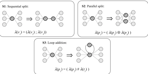
Finally, just like for Jackson nets we introduce rules that associate simple types with input-output graphs. The rules are given in Figure 10. The rules may be applied to any node in the input-output graph and the after each rule the new input and output sets are the same except that

• after S1 if v1 was an input node then v2is an input nodes,

• after S1 if v1 was an output node then v3 is an output node,

• after S2 if v1 was an input node then v2and v3are input nodes,

• after S2 if v1 was an output node then v2 and v3 are output nodes,

• after S3 if v1 was an input node then v2is an input nodes, and

• after S3 if v1 was an output node then v2 is an output nodes.

The class of input-output graphs that can be generated from a simple type is called simple Jackson graphs. S1: Sequential split:

⇒

⇒

⇒

Figure 10: The generation rules for simple Jackson graphs

The two following properties can be shown for simple Jackson graphs with induction upon their generation:

• It does not contain loops.

• It has at least one input node and at least one output node.

• For every node it holds that (1) it is either an input node or there is a non-empty path to it to from an input node and (2) it is either an output node or there is a non-empty path from it to an output node.

Lemma 5.7. If two simple types τ and τ0 generate the same simple Jackson graph then τ and τ0 are algebraically equivalent.

Proof. The proof proceeds as follows. We consider only so-called normalized simple types which means that the algebraic identities are applied as rewrite rules such that (1) all brackets are moved to the right, i.e., we do not allow types of the form ((τ1; τ2); τ3), ((τ1⊕ τ2) ⊕ τ3) or

((τ1#τ2)#τ3) and (2) we assign some kind of G¨odel-number G(τ ) to every simple type τ and

allow (τ1⊕ τ2) only if τ2 is of the form (τ3⊕ τ4) and G(τ1) ≤ G(τ3) or if if τ2 is not of the form

(τ3⊕ τ4) and G(τ1) ≤ G(τ2). Then we show that with each simple Jackson graph there is exactly

one such simple type that generates it.

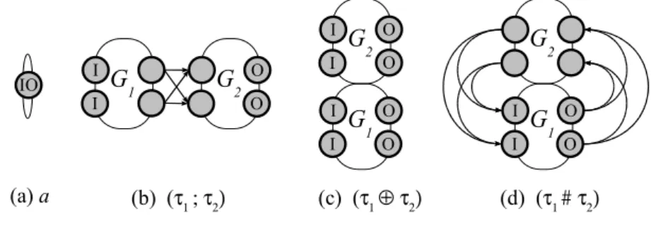
As discussed in the proof of Theorem 5.1 we can relate subexpressions of a simple type to subgraphs by considering the abstract syntax tree of the type. With this it can be shown that simple Jackson graphs can be decomposed into smaller simple Jackson graphs based on the type they were generated. These decompositions are schematically indicated in Figure 11 where (a) is the decomposition defined by an atomic type, (b) by a sequence type, (c) by a parallel type and (d) by an iteration type. Note that the input nodes and output nodes of the decomposed graph contain I and O, respectively. However, every simple Jackson graph can only be decomposed in one of these ways since with each decomposition certain properties of the graph must hold. For decomposition (a) the graph must contain exactly one node, whereas for all other decompositions there must be more. For decomposition (b) it must hold that from every input node there is a path to every output node, which is not true if decomposition (c) is possible since then there is no path from a node in G1 to a node in G2. For decomposition (d) the graph must be strongly

connected, which is not the case if (b) or (c) is possible since in both cases there is no path from a node in G2 to a node in G1. It follows that only one of the decompositions is possible for a

certain simple Jackson graph and hence all the simple types that generate it have the same form, i.e., the root node of the abstract syntax tree has the same label.

In the following we show with induction on the size of the simple Jackson graph that once we know the type of the root node of the syntax tree and the simple type that generates the simple Jackson graph is a normalized simple type then we can derive (1) what the type of the root node of G1is and (2) which part of the input-output graph is G1 and which part is G2.

First we consider the case where the root node of the abstract syntax tree indicates a sequence type. Since the type is normalized there are only three possibilities for the left-hand side and the corresponding decompositions are indicated in Figure 12. We can observe that decomposition (b.1) is characterized by a single input node, which is not possible for the other decompositions in the figure. Moreover, in (b.3) there are paths between all input nodes, which is not possible in (b.2). Once we know which decomposition applies we can derive what G1 (and therefore also

G2) as follows. For (b.1) G1 consists of the single input node. For (b.2) G1 consists of all the

nodes that are reachable from at least one of the input nodes but not from all of them. For (b.3) G1 consists of all the nodes that can be reached from an input node and from which we can

reach an input node.

Next we consider the case where the root node of the abstract syntax tree indicates an iteration type. Because the type is normalized we have also here only three possibilities for the left-hand side and the corresponding decompositions are indicated in Figure 13. We can observe that decomposition (d.1) is characterized by a single input node which is also an output node, which is not possible for (d.2) since there input nodes cannot be output nodes and also not for (d.3) since there we have at least two input nodes. Moreover, if we define internal paths as paths that, except for the first and last node, only go through nodes that are not input or output nodes, then in (d.2) there is between every input node and output node an internal path, whereas in (d.3) this is not possible. Also here we can derive what G1 (and therefore also G2) is since it

internal paths.

Finally we consider the case where the root node of the abstract syntax tree indicates a parallel type. If we assume that the type that generates the simple graph is (τ1⊕ (τ2⊕ . . . τk. . .))

with all τi not parallel types, then the k corresponding components can be found by taking the

finest partition of the nodes such that two nodes connected by an edge are in the same set. By induction we may assume that there is a unique normalized simple type for each component that generates that component, and the component with simple normalized type with the smallest G¨odel number has to be G1.

This concludes the cases to be considered, so it is in all cases uniquely determined how the simple Jackson graph has to be divided into component simple Jackson graphs, and by induction we may assume that for these components there is only one unique normalized simple type that generates them, and hence also only one that generates the complete simple Jackson graph.

IO I I

G

G

G

G

G

G

Figure 11: Decompositions of simple Jackson graphs based on their generating type

I

G

G

G

G

G

G

_G

Figure 12: Decompositions based on sequence types

Using Lemma 5.7 we can now prove Theorem 5.3.

Proof. We first show that two Jackson types τ and τ0generated the same Jackson net if τ and τ0 are algebraically equivalent. As was shown in the proof of Theorem 5.1 the graph of the place-expanded net is determined by the abstract syntax tree of the type such that for every leaf there is a node in the graph and there is an edge between two such nodes if the path between these nodes define a string in a certain regular language. It can then be shown that if an algebraic identity is applied to a syntax tree the string associated with two leaves is in that language iff

IO I I G_1.1 G_1.2O O I I O O G_1.2 G_1.1 O O I I G₂ (d.3) ((τ_1.1 ⊕ τ_1.2) # τ₂) (d.1) (a # τ2) G₂ (d.2) ((τ1.1 ; τ1.2) # τ2) G₂

Figure 13: Decompositions based on iteration types

it was before the identity was applied. It follows that the associated graph of the net stays the same if we apply an identity, and hence the whole Jackson net remains the same.

Next we show that if two Jackson types τ and τ0 generate the same Jackson net then τ and τ0 are algebraically equivalent. Assume that with an atomic Jackson net Ω we associate two Jackson types τ and τ0 and that these are not algebraically equivalent. With the Jackson type we can associate the simple types σ and σ0that are obtained by replacing || and + with ⊕. It can be shown that two Jackson types are algebraically equivalent iff the corresponding simple types are algebraically equivalent. It also holds that the graph of a Jackson net that is generated by a Jackson type is identical to the input-output graph that is generated by the simple type that is generated by the Jackson type. So it follows that σ and σ0 _{are not algebraically equivalent and}

hence that the graphs of the Jackson nets generated by τ and τ0 are not isomorphic. But this contradicts the assumption that τ and τ0 generate the same Jackson net, so the assumption that they are not algebraically equivalent must be false.

Summarizing, we can now characterize the ambiguity in the relationship between Jackson types and Jackson nets with the following corollary.

Theorem 5.8. If the Jackson nets Ω1 and Ω2 are generated by the Jackson types τ1 and τ2,

respectively, then the following are equivalent:

1. Ω1 and Ω2 are isomorphic

2. τ1≡alg τ2

Proof. Clearly (1) ⇒ (2) because if Ω1 and Ω2 are isomorphic then τ2 also generates Ω1 and so

by Theorem 5.3 it follows that τ1≡alg τ2. It also holds that (2) ⇒ (1) because if τ1≡algτ2then

by Theorem 5.3 there is a Jackson net Ω3generated by both τ1and τ2. Since both Ω1and Ω3are

generated by τ1, and both Ω2 and Ω3are generated by τ2it follows by Theorem 5.1 that Ω1and

Ω3are isomorphic, and Ω2 and Ω3are isomorphic. Hence Ω1 and Ω2 are also isomorphic.

5.3

Characterizing the expressive power of Jackson Nets

The set of Jackson nets is a proper subset of the set of workflow nets, which raises the question whether the class of workflows that they can express is not too limited. One way of comparing the expressive power of such formalisms is by looking at the sets of traces that can be expressed. These are in both cases the same, viz., if both places and transitions are labeled then both

formalisms can express exactly all sets of trances that can be described by Jackson types and if only places are labeled then both can express all regular languages. There is however a difference if we restrict ourselves to nets where each place and transition has a unique label. In that case the Jackson nets can only express trace sets that can be described by a Jackson type in which every atomic type appears at most once. Consider for example the net in Figure 8 which is not a Jackson net. Its trace set is described by the Jackson type (a; b; g; h) + (a; b; (((c; e; d)#f) k ((d; f; c)#e)); g; h) + (a; b; ((d#(f; c; e)) k (c#(e; d; f))); g; h). It can be verified that there is indeed no equivalent Jackson type where all the atomic types appear at most once. As is shown by Theorem 5.9 this is a characteristic property of trace sets that can be expressed by Jackson nets without duplicate labels, i.e., such Jackson nets can express exactly all trace sets that can be described by Jackson types in which every atomic type appears at most once. Moreover, as is shown in Corollary 5.13, this Jackson net is completely determined by the trace set, i.e., given a certain trace set there is at most one Jackson net without duplicate labels that represents this trace set. In the same corollary it is shown that it follows that for types in which atomic types appear at most once algebraic equivalence coincides with trace equivalence

Theorem 5.9. Let Ω be an atomic sound net without duplicate labels. Ω is a Jackson net iff there is an Jackson type τ in which every atomic type appears at most once and it holds that T r(τ ) = T r(Ω).

Before we prove this theorem we first prove the following lemmas.

Lemma 5.10. Let the atomic Jackson net Ω be generated by the Jackson type τ . All labels of Ω are different iff τ contains no duplicate labels

Proof. Let us define the number of occurrences of an atomic type a in a labeled Petri net as the sum of the number of times a appears in the label of each of the nodes of the net. It can be easily verified for each generation step Ωi⇒ Ωi+1 that an atomic type a occurs once in Ωi iff a occurs

once in Ωi+1. By induction it follows that for any generation sequence Ω0⇒ . . . ⇒ Ωk= Ω the

same holds for Ω0and Ωk. If this generation sequence associates τ with Ω then, since Ω0consists

of a single node labeled with τ , it holds that a occurs once in τ iff it does so in Ω0 and, as was

already shown, the latter is true iff a occurs once in Ωk = Ω.

Note that the fact that for each generation step Ωi ⇒ Ωi+1 an atomic type a occurs once

in Ωi iff a occurs once in Ωi+1, would not be true if we would use the Kleene-star in our types

instead of the # that we use now.

Lemma 5.11. If τ is a Jackson type without duplicate labels, Ω is a sound workflow net and T r(τ ) = T r(Ω) then Ω is safe, i.e., in all markings m that are reachable from the initial marking mi _{it holds that m(p) ≤ 1 for all places p in Ω.}

Proof. It can be shown with induction on the structure of τ that T r(τ ) does not contain a trace of the form xaay where x and y are strings of atomic types and a is an atomic type:

• If τ = B with B an atomic type then this clearly holds.

• If τ = (τ1; τ2) then we know by induction that aa does not appear in T r(τ1) or T r(τ2). So

if there is a trace of the form xaay in T r((τ1; τ2)) then T r(τ1) contains a trace of the form

xa and T r(τ2) contains a trace of the form ay. However, since every atomic type appears

only once in τ this is not possible.

• If τ = (τ1k τ2) then we know by induction that aa does not appear in T r(τ1) or T r(τ2).

So if there is a trace of the form xaay in T r((τ1k τ2)) then T r(τ1) contains a trace with a

and T r(τ2) contains a trace with a. However, since every atomic type appears only once