Optimization of compression techniques for still images and video for characterization of materials : mechanical applications

HAL Id: tel-02872875

https://tel.archives-ouvertes.fr/tel-02872875

HAL is a multi-disciplinary open access archive for the deposit and dissemination of sci-entific research documents, whether they are pub-lished or not. The documents may come from teaching and research institutions in France or abroad, or from public or private research centers.

L’archive ouverte pluridisciplinaire HAL, est destinée au dépôt et à la diffusion de documents scientifiques de niveau recherche, publiés ou non, émanant des établissements d’enseignement et de recherche français ou étrangers, des laboratoires publics ou privés.

Tarek Saad Omar Eseholi

To cite this version:

Tarek Saad Omar Eseholi. Optimization of compression techniques for still images and video for characterization of materials : mechanical applications. Signal and Image processing. Université de Valenciennes et du Hainaut-Cambresis, 2018. English. �NNT : 2018VALE0047�. �tel-02872875�

Pour obtenir le grade de Docteur de

L’UNIVERSITÉ POLYTECHNIQUE HAUTS-DE-FRANCE

Présentée et soutenue par : Tarek Saad Omar ESEHOLI Le 17/12/2018, à Valenciennes

Ecole doctorale : Sciences Pour l’Ingénieur (ED SPI 072)

Equipe de recherche, Laboratoire : Institut d'Electronique de Microélectronique et de

Nanotechnologie - Département Opto-Acousto-Electronique (IEMN DOAE – UMR 8520)

Optimisation des techniques de compression d’images fixes et

de vidéo en vue de la caractérisation des matériaux :

Applications à la mécanique

JURY Président de jury ;

M. Yannis POUSSET, Professeur des Universités, Laboratoire XLIM-SIC UMR 7252, Poitiers.

Rapporteurs :

M. Pierre Emmanuel MAZERAN, Maître de Conférences HDR, UTC, Laboratoire ROBERVAL UMR 7337, Compiègne.

Examinateurs :

Mme Anne-Sophie DESCAMPS, Maître de Conférences, Laboratoire IETR UMR 6164, Nantes.

M. Maxence BIGERELLE, Professeur des Universités, UPHF, Laboratoire

LAMIH UMR 8201, Valenciennes.

Directeur de Thèse :

M. Patrick CORLAY, Professeur des Universités, UPHF, Laboratoire IEMN DOAE UMR 8520, Valenciennes.

Co-Directeur de Thèse :

M. François-Xavier COUDOUX, Professeur des Universités, UPHF, Laboratoire

IEMN DOAE UMR 8520, Valenciennes.

Membres Invités :

Mme Delphine NOTTA, Maître de Conférences, UPHF, Laboratoire LAMIH UMR 8201, Valenciennes.

iii

Acknowledgements

“Say: Are those equal, those who know and those who do not know?” The Noble Quran [39 :9].

I would like to dedicate this work to spirit of my pure mother.

It is a pleasure to thank my supervisors Prof. Patrick CORLAY and Prof. François-Xavier COUDOUX for their guidance and encouragement.

I would like to thank my PhD. thesis jury members: my reviewers Prof. Yannis POUSSET, Prof. Pierre Emmanuel MAZERAN, as well as my examinators Mme Anne-Sophie DESCAMPS, Mme Delphine NOTTA, and Prof. Maxence BIGERELLE, for their time to review this manuscript and for their valuable remarks and comments which rich my work.

My father, thanks for your support and unconditional love. You can take all the credit for much of what I have achieved and what I will achieve in the future.

I would also like to thank Libyan Research, Science and Technology Authority for their financial support.

I would like to thank my colleagues and brothers in IEMN and LAMIH laboratories for their help and love.

I would like to thank Prof. Maxence BIGERELLE and Mme Delphine NOTTA for their time and patience to explain me the mechanical engineering concepts and techniques used in this research.

This thesis would have never been possible without my family Reima, Bailasan and Mohammed as well as my brothers, Sokina, Hesham, Salah and Bothina and their loving kids.

To all of you, I shall be forever indebted

Tarek Saad Omar Eseholi January 2019

v

Cette thèse porte sur l’optimisation des techniques de compression d'images fixes et de vidéos en vue de la caractérisation des matériaux pour des applications dans le domaine de la mécanique, et s’inscrit dans le cadre du projet de recherche MEgABIt (MEchAnic Big Images Technology) soutenu par l’Université Polytechnique Hauts-de-France. L’objectif scientifique du projet MEgABIt est d’investiguer dans l’aptitude à compresser de gros volumes de flux de données issues d’instrumentation mécanique de déformations à grands volumes tant spatiaux que fréquentiels. Nous proposons de concevoir des algorithmes originaux de traitement dans l’espace compressé afin de rendre possible au niveau calculatoire l’évaluation des paramètres mécaniques, tout en préservant le maximum d’informations fournis par les systèmes d’acquisitions (imagerie à grande vitesse, tomographie 3D). La compression pertinente de la mesure de déformation des matériaux en haute définition et en grande dynamique doit permettre le calcul optimal de paramètres morpho-mécaniques sans entraîner la perte des caractéristiques essentielles du contenu des images de surface mécaniques, ce qui pourrait conduire à une analyse ou une classification erronée. Dans cette thèse, nous utilisons le standard HEVC (High Efficiency Video Coding) à la pointe des technologies de compression actuelles avant l'analyse, la classification ou le traitement permettant l'évaluation des paramètres mécaniques. Nous avons tout d’abord quantifié l’impact de la compression des séquences vidéos issues d’une caméra ultra-rapide. Les résultats expérimentaux obtenus ont montré que des taux de compression allant jusque 100 :1 pouvaient être appliqués sans dégradation significative de la réponse mécanique de surface du matériau mesurée par l’outil d’analyse VIC-2D. Finalement, nous avons développé une méthode de classification originale dans le domaine compressé d’une base d’images de topographie de surface. Le descripteur d'image topographique est obtenu à partir des modes de prédiction calculés par la prédiction intra-image appliquée lors de la compression sans pertes HEVC des images. La machine à vecteurs de support (SVM) a également été introduite pour renforcer les performances du système proposé. Les

vi

robuste pour la classification de nos six catégories de topographies mécaniques différentes basées sur des méthodologies d'analyse simples ou multi-échelles, pour des taux de compression sans perte obtenus allant jusque 6: 1 en fonction de la complexité de l'image. Nous avons également évalué les effets des types de filtrage de surface (filtres passe-haut, passe-bas et passe-bande) et de l'échelle d'analyse sur l'efficacité du classifieur proposé. La grande échelle des composantes haute fréquence du profil de surface est la mieux appropriée pour classer notre base d’images topographiques avec une précision atteignant 96%.

Mots-clés : Big Data – mécanique - science des matériaux - compression et analyse

des données - traitement de l'information - codage vidéo à haute efficacité (HEVC) - machine à vecteurs de support (SVM).

vii

Abstract

This PhD. thesis focuses on the optimization of fixed image and video compression techniques for the characterization of materials in mechanical science applications, and it constitutes a part of MEgABIt (MEchAnic Big Images Technology) research project supported by the Polytechnic University Hauts-de-France (UPHF). The scientific objective of the MEgABIt project is to investigate the ability to compress large volumes of data flows from mechanical instrumentation of deformations with large volumes both in the spatial and frequency domain. We propose to design original processing algorithms for data processing in the compressed domain in order to make possible at the computational level the evaluation of the mechanical parameters, while preserving the maximum of information provided by the acquisitions systems (high-speed imaging, tomography 3D). In order to be relevant image compression should allow the optimal computation of morpho-mechanical parameters without causing the loss of the essential characteristics of the contents of the mechanical surface images, which could lead to wrong analysis or classification. In this thesis, we use the state-of-the-art HEVC standard prior to image analysis, classification or storage processing in order to make the evaluation of the mechanical parameters possible at the computational level. We first quantify the impact of compression of video sequences from a high-speed camera. The experimental results obtained show that compression ratios up to 100: 1 could be applied without significant degradation of the mechanical surface response of the material measured by the VIC-2D analysis tool. Then, we develop an original classification method in the compressed domain of a surface topography database. The topographical image descriptor is obtained from the prediction modes calculated by intra-image prediction applied during the lossless HEVC compression of the images. The Support vector machine (SVM) is also introduced for strengthening the performance of the proposed system. Experimental results show that the compressed-domain topographies classifier is robust for classifying the six different mechanical topographies either based

viii

ratios up to 6:1 depend on image complexity. We evaluate the effects of surface filtering types (high-pass, low-pass, and band-pass filter) and the scale of analysis on the efficiency of the proposed compressed-domain classifier. We verify that the high analysis scale of high-frequency components of the surface profile is more appropriate for classifying our surface topographies with accuracy of 96 %.

Keywords: Big Data - Mechanics, Materials Sience - Data Compression and analysis -

ix

TABLE OF CONTENTS

LIST OF FIGURES ………..XII LIST OF TABLES………XVI

CHAPTER 1 INTRODUCTION ... 1

1.1 Context and Motivation ... 1

1.2 Challenges ... 3

1.3 Contributions... 4

1.4 Structure of the Manuscript ... 5

CHAPTER 2 STATE-OF-THE-ART ... 7

2.1 Digital Images and Video Compression ... 7

2.1.1 Basics of Image Compression Techniques ... 8

2.1.2 Illustrative Example of the JPEG Still Image Compression Standard ... 14

2.1.3 Motion Compensation and Video Compression ... 17

2.2 Material Surface Engineering ... 22

2.2.1 Surface Topography ... 22

2.2.2 Surface Topography Measurement ... 25

2.2.3 Mechanical Image Deformation Analysis ... 26

2.2.4 Surface Topographical Images Classification ... 30

2.3 Support Vector Machine (SVM) ... 33

2.3.1 Mathematical Linear SVM ... 34 2.3.2 Nonlinear SVM ... 37 2.3.3 K-Fold Cross-Validation ... 40 2.3.4 Multiclass SVM ... 41 2.3.4.1 One-Against-All (OAA) ... 41 2.3.4.2 One-Against-One (OAO) ... 41

x

CHAPTER 3 HIGH EFFICIENCY VIDEO CODING (HEVC) ... 43

3.1 Improvements in HEVC Coding Stages ... 43

3.2 HEVC Intra Prediction Coding ... 47

3.3 Lossless Coding ... 52

3.4 High Bit Depth Still Picture Coding ... 53

3.5 Conclusion ... 53

PERFORMANCE EVALUATION OF STRAIN FIELD MEASUREMENT CHAPTER 4 BY DIGITAL IMAGE CORRELATION USING HEVC COMPRESSED ULTRA-HIGH-SPEED VIDEO SEQUENCES. ... 55

4.1 Context of the study ... 55

4.2 Methodology ... 56

4.3 Methods and Materials ... 56

4.3.1 High-speed test device ... 56

4.3.2 HEVC Lossy and Lossless Compression ... 58

4.4 Results ... 59

4.4.1 Tensile Test of Polypropylene (PP) Specimen ... 59

4.4.2 Sikapower Arcan test ... 60

4.4.3 Discussion... 61

4.5 Conclusion ... 73

CHAPTER 5 SVM CLASSIFICATION OF MULTI-SCALE TOPOGRAPHICAL MATERIALS IMAGES IN THE HEVC-COMPRESSED DOMAIN ... 75

5.1 Context of the study ... 75

5.2 Methodology ... 76

5.2.1 Methods and Materials ... 77

5.2.2 Surface Processing ... 77

5.2.3 Topographical Materials Texture Image Dataset ... 78

5.2.4 IPHM-Based Classification ... 79

5.2.5 HEVC Lossless 4x4 PU Compression ... 83

5.2.6 SVM Classification ... 83

5.3 Results ... 84

5.3.1 The Impact of Surface Topography Filtering Types on Achieved Compression Ratios………..85

xi

Classification Accuracy ... 89

5.3.4 The Impact of Scale of Analysis on Topographical Images Classification Accuracy………95

5.4 Conclusion ... 99

CHAPTER 6 CONCLUSION AND PERSPECTIVES ... 100

xii

LIST OF FIGURES

Figure 2-1 Mobile video will represent 78% of the world’s mobile data traffic by 2021,

according to Cisco [18]……….………7

Figure 2-2 Representation of a digital video signal……….…….…………9

Figure 2-3 The general image compression framework [23]……….……….11

Figure 2-4 Simplified block diagram of the JPEG DCT-based encoder [38]……….15

Figure 2-5 Classic motion-compensated codec scheme………...……..18

Figure 2-6 Block matching algorithm [16]……….18

Figure 2-7 MPEG GOP example.………...19

Figure 2-8 Pictorial display of surface texture [51] ...………24

Figure 2-9 Schematic Diagram of Stylus Instrument [52]……….……….25

Figure 2-10 Sample of LAMIH topographical image databases with size of [1024x1024 16-bit depth]………..26

Figure 2-11 A schematic of the DIC system.………..28

Figure 2-12 Corresponding relation of deformed and undeformed sub-image.………...…..29

Figure 2-13 The optimal separation hyperplane (OSH)………..35

Figure 2-14 Transformation of the data set by Φ [104]……….38

Figure 2-15 5-Fold Cross-Validation [106]………....40

Figure 3-1 Structure of HEVC encoder and decoder (with elements shaded in light gray) [110].43 Figure 3 2 HEVC Intra/Inter partitioning modes of a CU to PUs [49], [112]………45

Figure 3-3 Example for the partitioning of a 64x64 coding tree unit (CTU) into coding units (CUs) with different coding depths……….46

Figure 3-4 (a) HEVC intra-prediction modes (b) Prediction principle for 4x4 PU [119]...…….48

Figure 3-5 The reference sample locations relative to the current sample for Horizontal and Vertical angular intra prediction (with positive and negative prediction angles) respectively ( the idea is [121] )………..49

Figure 3-6 Representation of the Planar prediction……….…...51

Figure 4-1 Reference image for 2D-DIC specimen measurements with Subset size of 18×18 pixels………...57

xiii

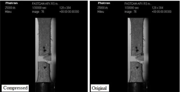
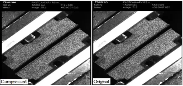
512x472 pixels vs. useful part of 128x384 pixels)……….60 Figure 4-3 First image at undeformed stage of Arcan test at 45° of Sikapower glue joint……....61 Figure 4-4 R-D curves for the two video sequences………..63 Figure 4-5 Illustration of HEVC high quality performances for compressed sequence1 (QP=25, PSNR =44.4dB and SSIM=0.99) compared with the original sequence1………..63 Figure 4-6 Illustration of HEVC high quality performances for compressed sequence2 (QP=25, PSNR =39.2dB and SSIM=0.98) compared with the original sequence2………..64 Figure 4-7 Evolution of relative gaps on computed axial strain throughout tensile loading of PP - Case Lossy - QP0 (All data)………...66 Figure 4-8 Evolution of relative gaps on computed axial strain throughout tensile loading of PP - Case Lossy - QP0 (Focus on relative gaps between -10% and 10%...66 Figure 4-9 Evolution of relative gaps on computed axial strain throughout tensile loading of PP - Case Lossy - QP5 (All data) ………...67 Figure 4-10Evolution of relative gaps on computed axial strain throughout tensile loading of PP - Case Lossy - QP5 (Focus on relative gaps between -10% and 10) ………...….67 Figure 4-11 PP - Case Lossy - QP20 (All data) ……….68 Figure 4-12 Evolution of relative gaps on computed axial strain throughout tensile loading of PP - Case Lossy - QP20 (Focus on relative gaps between -10% and 10%) ……...………68 Figure 4-13 Evolution of relative gaps on computed axial strain throughout tensile loading of PP - Case Lossy - QP25 (All data) ………....69 Figure 4-14 Evolution of relative gaps on computed axial strain throughout tensile loading of PP - Case Lossy - QP25 (Focus on relative gaps between -10% and 10%)………...………69 Figure 4-15 Evolution of relative gaps between strains computed from Lossy images and Lossless images of Sequence 2 (Arcan shear test of glue joint), in the ZOI of maximal shear strain (Axial strain)………...………...70 Figure 4-16 Evolution of relative gaps between strains computed from Lossy images and Lossless images of Sequence 2 (Arcan shear test of glue joint), in the ZOI of maximal shear strain (Shear strain)………..71 Figure 4-17 Evolution upon loading of strains computed from Lossy images of Sequence 2 (Arcan shear test of glue joint), in the ZOI of maximal shear strain (Axial strain) ...………72

xiv

(Arcan shear test of glue joint), in the ZOI of maximal shear strain (Shear strain) ...………72 Figure 5-1 Nomenclature used to represent the collected mechanical topographic images….…..78 Figure 5-2 Represents one image (Resolution of 1024x1024 pixels) from six mechanical material categories, with two different zooming and three filtered images………..79 Figure 5-3 Original Image 512x512 (A), selected modes to predict the original image presented with 35 colors (B) Intra Predicted Image (C) and The Residual image (D)………...80 Figure 5-4 First five retrieved images for six images tests (categories 1 to 6) using IPMH, which indicate classification accuracy of 30 %...82 Figure 5-5 Block diagram depicting the procedure for learning and testing the SVM model.

………84 Figure 5-6 Relationship between the scale of analysis and the six surface categories compression performance by using the multi-scale LP-datasets……….85 Figure 5-7 Relationship between the scale of analysis and the six surface categories compression performance by using the multi-scale BP-datasets……….86 Figure 5-8 Relationship between the scale of analysis and the six surface categories compression performance by using the multi-scale HP-datasets……….87 Figure 5-9 Original Image 1024x1024 (A), selected modes to predict the original image presented with 35 colors (B) Intra Predicted Image (C) and The Residual image (D)………...87 Figure 5-10 Comparison between the IPMHs averages for three different filtered image data sets; LP, BP, and HP data set………..88 Figure 5-11 The effect of increasing the training set size on the classification accuracy while using mixed multi-scale HP, LP, and BP datasets………..89 Figure 5-12 The Confusion matrix for classifying the six surface categories (Mixed)…………..90 Figure 5-13 The effect of increasing the training set size on the classification accuracy while using HP- datasets………...90 Figure 5-14 Confusion matrix for six surface categories classification by using 60 % of multi-scale HP data set for training………..91 Figure 5-15 The relation between the size of the training data set and the six surface categories classification performance by using the mixed multi-scale LP- datasets………...92 Figure 5-16 Confusion matrix for six surface categories classification by using 60 % of multi-scale LP data set for training………...92

xv

classification performance by using the mixed multi-scale BP-datasets………93 Figure 5-18 Confusion matrix for six surface categories classification by using 60 % of

multi-scale BP data set for

training………....94

Figure 5-19 The relation between the scale of analysis and the six surface categories compression and classification performance by using the multi-scale LP-datasets……….….95

Figure 5-20 The relation between the scale of analysis and the six surface categories compression and classification performance by using the multi-scale BP-datasets………..…96

Figure 5-21 The relation between the scale of analysis and the six surface categories compression and classification performance by using the multi-scale HP-datasets………..…97

Figure 5-22 Confusion matrix for six surface categories classification by using 60 % of

highest-scale HP data set for

xvi

LIST OF TABLES

Table 3-1 Displacement Angle corresponding to Angular prediction Mode [41]. ... .48 Table 4-1 HM 10.1 Encoder Parameters ... 58 Table 4-2 HEVC Compression Performances ... 62

xvii

LIST OF ACRONYMS

AVC Advanced Video Coding

ANNs Artificial Neural Networks

bpp bits per pixel

CABAC Context Adaptive Binary Arithmetic Coding

CBR Constant Bit Rate

CT Computed Tomography

CTU Coding Tree Unit

CU Coding Unit

DCT Discrete Cosine Transform

DFT Discrete Fourier Transform

DIP Digital Image Processing

DPCM Differential Pulse Code Modulation

DST Discrete Sine Transform

GOP Group of Pictures

HEVC High-Efficiency Video Coding

HM HEVC test Model

HVS Human Visual System

xviii

IEC International Electrotechnical Commission

ISO International Standard Organization

ITU-T International Telecommunication Union

i2i integer-to-integer

JPEG Joint Photographic Experts Group

JVT Joint Video Team

KLT Karhunen-Loeve Transform

LCU Large Coding Unit

MAD Mean Absolute Difference

MSE Mean Square Error

PPS Picture Parameter Set

PSNR Peak Signal to Noise Ratio

PCM Pulse Code Modulation

PU Prediction Unit

QP Quantization Parameter

RDO Rate-Distortion Optimization

RExt Range Extension

RLE Run-Length Encoding

ROI Region of Interest

SAP Sample Adaptive intra-Prediction

SAP-G Sample-based Angular intra-Prediction with Gradient-based

SAP-ME Sample-based Angular intra-Prediction with Median and Edge

SWP Sample-based Weighted Prediction

SAO Sample Adaptive Offset

SSIM Structural Similarity Index

SVM Support Vector Machine

TU Transform Unit

xix

VQA Video Quality Assessment

CHAPTER 1

INTRODUCTION

Context and Motivation

During the last decade, several advanced technological techniques emerged in the fields of material science engineering that allow establishing the links between the structure, dynamics and functioning of materials [1], [2]. Materials science engineering studies the characteristics of materials: biological, chemical, physical, optical, and mechanical properties. The mechanical properties are defined from the surface topography when exposed to different types of loads and stresses such as tension, compression, bending, torsion and drawing at micro- or nanometer scale dimensions [3], [4]. This analysis scale is recommended for: aquistition and analysis of material surface for improving the understanding of material surface functionality [5], [6]. Surface topography or surface texture is one of the most relevant characteristics of any material surface that has widely exploited in many mechanical machining processes such as: grinding, shaping and milling [7]. Indeed, several imaging methods for characterizing the physical-mechanical properties exist including advanced optical and scanning electron microscopy, X-ray imaging, spectroscopy, high-speed imaging, electron or micro-topography. Topography measurement systems allow us to obtain specific images for the surface particles represented in three dimensions: height, width, and depth ( surface profile) [8]. Obviously, many of these material imaging techniques generate big image databases with high spatial and temporal resolution, large size and pixel depth, which represent a significant amount of data to be stored or transmitted [4], [9]. It would be of great interest to apply lossy or lossless compression prior to classify or store images, where the decompressed image is used as an input for any image processing material algorithm [9]–[11]. Unfortunately, compression artifacts introduced by these algorithms not only affect the visual quality of an image but can also distort the features that one computes for subsequent tasks related to image analysis or pattern recognition in material science

engineering. Since imaging technologies are widely used to analyze the mechanical properties of materials, considering the image quality is essential. The reason behind is that the materials properties is largely dependent on microstructures, which could be affected if the decompressed image is different from the original one. Materials science engineering is a scientific field that requires the acquisition, processing, and analysis of a tremendous amount of image and video information data [12]. Today, the two main topics in material surface imagery fields are: (1) Measuring the similarity or matching between two surface topographies images for comparing the characteristics of two different engineering surfaces. Surface similarity measurement is a promising operation for solving many problems in different material engineering fields such as: industrial surface inspection, defect detection, remote sensing, material classification and biomedical image analysis [13], [14]. (2) Determining which surface filtering range and analyse scale should be used for multi-scale surface topography analyzing and classification. Multi-scale surface filtering decomposition techniques have proven their efficiency in roughness functional analysis [15]. It decomposes the surface topography profile into three different filtered images: high-pass (HP), low-pass (LP) and band-pass (BP) filtered images, which represent the surface roughness, the primary form, and the waviness, respectively. Most of previously surface engineering studies were based on roughness which is represented by the high frequency (HP) component of surface profile.

This thesis addresses the challenges of MEgABIt (MEchAnic Big Images Technology) project. MEgABIt is a project that aims to measure the surface topography and study the surface functionality in the compressed-domain in order to reduce the computation cost. The MEgABIt database is composed of high-resolution 8-bpp and16-bpp images of size 1024x1024 pixels. The similarity between image pairs in the database is too high to the extent that makes the classification problem very challenging.

 The objectives of this thesis are:

1. Study the impact of HEVC (lossless and lossy) compression on the characterization of material mechanical response image sequences for crash and impact loading processes captured by an ultra-high-speed camera.

2. Evaluate the impact of the HEVC lossy and lossless compression algorithms by: (1) Analyzing the mechanical loading response by Vic-2D Software after applying HEVC compression techniques. (2) Considering the compression ratios as well as the quality of the reconstructed video.

3. Implementing HEVC lossless compression algorithm to evaluate the impact of surface filtering types and the scale of analysis on the compression and classification efficiency by considering the compression ratios as well as the classification accuracy for different study conditions.

Challenges

1. The processing task is very challenging when considering mechanical image databases of high-bit resolution, high frame rate, large size and pixel depth, which represent a big amount of data in terms of storage, analysis, classification or transmission over networks.

2. Using lossless compression techniques compression ratio results is limited (or reduced) compared with lossy compression techniques. However, lossy compression techniques give high compression ratios that could cause the loss of the essential characteristics in the mechanical surface image, which leads to wrong analysis or classification. Therefore, we should smartly select the CR for the lossy techniques in order to preserve the original mechanical contents needed for mechanical analysis.

3. Multi-scale surface topographies classification is difficult because the topographical image feature descriptors must be invariant to transformation of surface images like filtering range of surface profile and scale of analysis.

4. Images are stored and transmitted in compressed form. So, they have to be reconstructed prior to be analyzed or classified. This process might be time consuming for retrieval and classification applications.

Contributions

In this work, we implemented HEVC compression standard to reduce the computation complexity of analysis and classification of mechanical surface topographies. The internal bit depth is extended to 16-bpp and the prediction unit is fixed to the size of to 4x4 samples block to enhance the quality of the extracted features for accurate mechanical response image analysis and classification. Our contributions can be summarized in the following points:

1. We evaluate the effect of HEVC lossy and lossless compression on characterizing

material surface mechanical response when subject to severe loading conditions over a wide range of strain rates. The impact of HEVC compression was evaluated by analyzing the compressed mechanical loading response sequences by Vic-2D Software. In addition, we evaluated the efficiency of the proposed compression techniques by considering the compression ratios as well as the quality of the reconstructed video. After using two different image sequences, the results demonstrated that HEVC provided very high coding efficiency as well as high visual quality. In addition to that, we succeeded to retrieve the original mechanical data from the HEVC compressed sequences at Quantization Parameter ranging from 0 to 20 as indicated after analyzis of mechanical response using the Digital Image Correlation (DIC) software.

2. We evaluated the effects of surface filtering types and the scale of analysis on the

efficiency of the proposed lossless compressed-domain topographical images classifier by considering the compression ratios as well as the classification accuracy for different study conditions. Each surface profile was decomposed into three multi-scale filtered image types: high-pass HP, low-pass LP, and band-pass BP filtered image datasets. Furthermore, the collected database was lossless compressed using HEVC, then the compressed-domain Intra Prediction Mode Histogram (IPMH) feature descriptor was extracted from each predicted image. Simultaneously, we need to keep the visual quality good for visual analysis of mechanical image by experts.

3. We used the support vector machine (SVM) algorithm to classify the high similarity

image pairs of the collected topographical image databases (LAMIH databases), i.e. decide if they were taken either from the same category or from different categories.

The model has evaluated 13608 multi-scale topographical images by considering the compression ratios as well as the classification accuracy for each study condition. The experimental results showed that robust compressed-domain topographies classifier was either based on single or multi-scale analyzing methodologies. The high-frequency components (HP-dataset) of the surface profile were the most appropriate for characterizing our surface topographies with achieved accuracy of 96 %.

Structure of the Manuscript

This thesis is organized as following: Chapter 2 reviews the proposed approaches in the literature for: Firstly, the basics of image and video compression including a brief explanation about digital image and video compression including JPEG, motion compensation and video compression. Secondly, we briefly explain the fundamentals of mechanical surface measuring, analyzing and classification. Thirdly, we give the SVM basics: linear, non-linear and the extension of the binary SVMs to the multiclass case.

Chapter 3 presents the fundamentals of the state-of-the-art HEVC digital video

coding standard. We mention the main enhancements introduced to HEVC standard compared to previous coding solutions like Intra Prediction coding technique, or high-bit depth still-image compression. We detail our contribution to improve HEVC lossy and lossless techniques by fixing the prediction unit to 4x4 samples and increasing the internal bit depth to 16 bits.

Chapter 4 describes the implementation of our proposed methods for testing the

influence of image compression on mechanical response analysis as well as presenting the obtained results.

Chapter 5 presents an original method based on the SVM algorithm for multi-scale surface

classification in the compressed domain. In the experimental results we discuss the effect of surface filter type and scale of analysis on the compression and the classification accuracy.

CHAPTER 2

STATE-OF-THE-ART

Digital Images and Video Compression

Digital images and videos constitute the first pillar of multimedia technologies like broadcast TV, online gaming, mobile communications or multimedia streaming [16]. Every minute, a huge amount of images and videos is created in a great number of domains such as medical imaging, entertainment, earth monitoring or industrial applications [9]. Indeed, telecom operators like Cisco or Nokia predict that video traffic will represent about 80% of all consumer Internet traffic in the coming years [17].

Figure 2-1 Mobile video will represent 78% of the world’s mobile data traffic by 2021, according to Cisco [18].

Consequently, the processing, storage and transmission of images and videos over networks constitute a very challenging task. In order to overcome such problem, several digital image and video compression techniques have been developed during the last twenty years in order to reduce the image and video data size while keeping good video quality. In what follows, we first introduce the basics of image and video compression. Then we describe the JPEG still image compression standard, as an illustrative example. Finally, we describe motion estimation/compensation technology and give an overview of first-generation video compression standards.

2.1.1 Basics of Image Compression Techniques

Digital image and video compression is the science of coding the image content to reduce the number of bits required in representing it, aiming facilitate the storage or transmission of images with a level of quality required for given application (digital cinema, mobile video streaming) [19]. Typically, a digital image signal contains visual information in a two-dimensional matrix of size equal to N rows by M columns. Each spatial sample also known as a pixel is represented digitally with a finite number of bits called bit-depth [20].

For example, each pixel in a grayscale image is typically represented by a byte word, i.e. 8 bit-depth. A standard RGB color image is represented by three byte words, i.e. 24 bit-depth corresponding to 8 bits for the red component, 8 bits for the green one, and 8 bits for the blue one [21].

Digital video signals are represented as a collection of successive still images separated by a fixed interval time, which determines the so-called frame rate [16].

The compression process can be performed by exploited many duplicated information in the digital image or video signals. For example, it is possible to exploit the fact that the human eye is more sensitive to brightness than color for reducing the size of an image. To do that, the RGB components of the color image are first converted into the three YUV color components, where Y corresponds to the luminance (brightness) and U and V are the chrominance components, respectively. Then, the chrominance components are usually reduced by a factor of 1,5 or 2 by appropriate spatial down sampling [22].

Figure 2-2 Representation of a digital video signal.

For instance, a high-definition broadcast video signal typically consists in a sequence of successive frames at a frame rate of 25 fps. Each frame corresponds to a matrix of

1920x1080 pixels with 4:2:0 sample format (i.e. 1920x1080 luminance samples and 960x540 samples for each chrominance component), and 8 bit-depth precision. Hence, the corresponding bit rate around 620 Mbit /s.

Indeed, chroma subsampling does not reduce the image data size in a sufficient way and other compression operations are needed to fulfill bandwidth constraints. Efficient image and video compression can be achieved by eliminating two main types of redundancies known as statistical redundancy and psychovisual redundancy [16], [19], [20], [23]:

 Statistical Redundancy can be divided into two categories:

o first, the pixel-to-pixel redundancy traduces the correlation which exists between pixels both in the spatial and temporal domains:

- Spatial redundancy is related to statistical correlation between the intensity values of neighbor pixels very closed to each other. Spatial redundancy can be eliminated using the differential coding or intra-predictive coding.

- Temporal redundancyis related to the statistical correlation between pixels belonging to two successive video frames, which is as high as the time interval between two consecutive video frames is short. Often, this kind of redundancy can be eliminated using inter-predictive coding between consecutive frames.

o The Coding Redundancy is coming from the information redundancy between coded symbols, it can eliminate by using so-called binary entropy coding techniques.

 Psychovisual Redundancy is based on the characteristics of the Human Visual System (HVS). Indeed, some visual informations are less relevant than others in a frame content due to so-called masking phenomenon which may occur in luminance, contrast, texture and frequency domain. Consequently, these irrelevant visual data can be suppressed without degrading visual quality. However, in this case, it should be noted that the reconstructed signal is mathematically different from the original one.

In fact, digital image compression techniques are broadly classified into two categories; Lossless (reversible) and Lossy (or irreversible) compression techniques [20], [21], as generalized in Figure 2-3.

Figure 2-3 The general image compression framework [23].

The Lossless image compression category is widely used in specific-imagery

applications requiring the reconstructed image to be exact compared to the original one, such as medical imaging, document archiving and scientific imagery. Here, the decoder is perfect inverse of the encoding process and the original image can be fully retrieved from the compressed file. However, the so-called compression ratio remains moderate ranging from 2:1 to 10:1 on average, based on image complexity [24]. Here, the compression ratio (CR) is defined as the ratio of the size of the original image in bits, to the size of the compressed stream expressed also in bits:

Compression Ratio (CR) =_{Total number of bits in the compressed image}Total number of bits in the original image (2.1)

For example, CR=2:1 means that the compressed file is twice as small as its original version. The spatial redundancy is reduced in the decorrelation stage by using the prediction-based methods [21], [25], or transform-prediction-based methods such as discrete cosine transform DCT [26] or the reversible wavelet transformation (DWT) [27]. Followed by Entropy coding for

reducing the coding redundancy. The number of bits required to represent a sequence of symbols is reduced to a minimum length as in binary arithmetic coding, Huffman Coding and Variable-length Coding [28].

The Lossy image compression category allows achieving higher compression ratios (up

to more than 100:1) while losing part of image information. Further, the reconstructed image will not be mathematically identical to the original image, so it is necessary to determine the minimum data required for retrieving all necessary information [24]. The spatial redundancy is reduced by using one of the existing pixel decorrelation techniques as predictive coding, transform coding, sub-band coding [29]. The residual of transform data is computed and subject to an additional non-reversible process known as quantization to increase significantly coding efficiency. Finally, the quantized coefficients are lossless compressed by entropy coding [19]–[21], [25], [30], [31].

The optimal compression scheme will be able to obtain the highest compression ratio as well as best image quality with least computation complexity.

In the case of lossless compression, there is no distortion, so the reconstructed image is mathematically and by consequence visually identical to the original one. In the case of lossy compression, however, there is a need to additionally measure decoded image quality as well as the achieved CR [21].

Digital image quality can be evaluated both subjectively and objectively [29], [32].

 The subjective quality measurement is based on observations performed by human viewers in a controlled test environment. Human viewers are asked to give a score to the processed images according to different quality or degradation scales [33]. Subjective tests represent the ground truth, but they are often time consuming and expensive. Hence, objective image and video quality metrics are frequently used because of their ease of implementation.

 The objective quality measurement is generally based on the image statistical properties and permits to evaluate the rate-distortion (RD) performances of digital image and video compression algorithms. Different quality metrics exist depending on the

knowledge or not of the original visual signal [34]. Among these, Full Reference (FR) quality metrics are calculated from the original image and its compressed version. The best-known FR objective video metric is undoubtedly the Peak Signal-to-Noise Ratio (PSNR). The PSNR metric, expressed in decibels, is defined as:

𝑀𝑆𝐸 (2.2)

Where the Mean Squared Error (MSE) is defined as:

𝑀𝑆𝐸 = _{M N}1 ∑ ∑𝑁 ⌊𝐼(𝑖, 𝑗) − 𝑅(𝑖, 𝑗)⌋ 2 𝑗=1

𝑀

𝑖=1 (2.3)

and

- I (i, j) represents the pixel value at position (i,j) in the original image of size MxN pixels.

- R (i, j) represents the pixel value at position (i,j) in the reconstructed image of same size.

- Maximum Pixel Intensity is equal to 255 for 8-bit resolution.

The higher PSNR value is, the better visual quality is. In the case of lossless compression, the PSNR value is equal to infinity. However, even if the PSNR metric is easy to use, it is well known that PSNR (or in an equivalent way, the MSE) is poorly correlated with the human visual judgment [35]. To overcome this problem, many other quality metrics derived from the PSNR have been proposed in the literature that try to mimic the Human Visual System (HVS) [29]. We can cite for example the Weighted Signal to Noise Ratio (WSNR), Noise Quality Measure (NQM) and Visual Signal to Noise Ratio (VSNR). The Structural Similarity Index, known as SSIM, and its variants constitute another alternative to the PSNR metric. SSIM is a full reference quality metric. It measures the visibility of any error in the structural information of the image and incorporates HVS properties like luminance and contrast masking. SSIM varies between 0 (poor quality) and 1 (perfect). It is commonly

accepted that SSIM clearly outperforms PSNR or MSE and SSIM is nowadays widely used by the image processing community.

To conclude about image quality evaluation, the term «image compression» should be understood in a mechanical application-specific sense in this thesis. This makes a great difference with “classical” image compression, where the decompressed images are intended to be viewed by a human observer. In this case, the quality of decompressed image is evaluated based on perceptual considerations obtained according to HVS properties.

In our work, the decompressed image is used as an input of an image processing algorithm. The decompressed image is not viewed by a human viewer, which makes unusable applying of considerations obtained according to HVS properties. In the present case, the error introduced by lossy compression should not affect the accuracy of information data extracted from the decompressed image that is needed for further material analysis or classification, while keeping high compression ratio. It is not strictly necessary that the decompressed image looks visually close to the original one. Rather, the decompressed image should contain as minimum information data as needed to guarantee material imaging processes of high quality.

2.1.2 Illustrative Example of the JPEG Still Image Compression Standard

The JPEG compression standard is one of the most well-known image compression standards. It takes its name from the working group called the Joint Photographic Expert Group that developed it in the early 1990s. Today, the JPEG standard is still widely used [26] in a broad range of digital imaging applications like digital photography, medical imaging, or video recording (using Motion JPEG) [26]. Moreover, it provides the basis for future standards including JPEG2000, and High Efficiency Video Coding (HEVC)-Intra. JPEG is designed to handle color and grayscale image compression with an achieved compression ratio of up to 1: 100 [36] . It is based on the Discrete Cosine Transform (DCT) which analyses the image as the human eye does. The human eye does not see all the colored details present in the image, consequently the fine details corresponding to high spatial frequencies can be removed with no effect for the human viewer [37]. The encoding process is started by

dividing the original image into squared blocks of 8x8 samples. Each block is transformed by Forward DCT or DCT from the pixel domain to the frequency domain in order to reduce the spatial redundancy. After DCT, the block energy is generally concentrated in few low frequency transform coefficients. Then, the 64 DCT coefficients are quantized hence reducing the number of non-null values. Finally, the quantized coefficients are sent to the entropy coder that delivers the output stream of compressed image data as illustrated in Figure 2-4.

Figure 2-4 Simplified block diagram of the JPEG DCT-based encoder [38].

The main JPEG encoding process steps are briefly illustrated below:

1. Block segmentation: the full compression of the image makes non-ideal compression

results. For this reason, JPEG standard suggests that image is dividing into 8x8 blocks and starting from this stage each of these 64-pixel blocks is processed separately at all codec stages.

2. Discrete Cosine Transform (DCT): transforming each block of 8x8 pixels into the

spatial frequency domain allows the algorithm to ignore less critical pixels of the original block by removing the inter-pixel redundancy inside the original image. This process makes the quantization process easier to know which parts of the block are less important. Typically, the highest AC coefficients are deleted during the quantization process. JPEG calculates the Forward Discrete Cosine Transform (FDCT) and Inverse Discrete Cosine Transform (IDCT) by two following equations [38]:

FDCT: 𝑆𝑣𝑢= 1₄ 𝐶𝑢 𝐶𝑣 ∑7𝑥=0∑7𝑦=0𝑆𝑦𝑥cos(2𝑥+1)𝑢𝜋₁₆ cos(2𝑦+1)𝑣𝜋₁₆ (2.4)

IDCT: 𝑆𝑦𝑥 = 1₄ ∑7𝑢=0∑7𝑣=0 𝐶𝑢 𝐶𝑣 𝑆𝑣𝑢𝑐𝑜𝑠(2𝑥+1)𝑢𝜋₁₆ 𝑐𝑜𝑠(2𝑦+1)𝑣𝜋₁₆ (2.5)

where: 𝐶𝑢, 𝐶𝑣 = 1⁄_√2 For u, v =0

𝐶_𝑢, 𝐶_𝑣 = 1 Otherwise

3. Quantization: the quantization stage is centered at the core of any lossy encoding

algorithm for reducing the psychovisual redundancy. It is a non-reversible operation, and it must be bypassed in lossless compression mode [19], [31], [37], [39], [40]. In order to remove the less significant DCT coefficients in the transformed block, every element in the 8x8 FDCT matrix 𝑆𝑉𝑈 is divided by a corresponding step size 𝑄𝑉𝑈 from a previously

calculated 8x8 quantization table (Q-table) [23] and rounded to the nearest integer as shown in Eq. (2.6):

𝑆𝑞_𝑣𝑢= 𝑟𝑜𝑢𝑛𝑑 ( _𝑄 𝑆𝑣𝑢

𝑣𝑢) (2.6)

Moreover, the magnitude of the non-zero coefficient values is limited after division and rounding to smaller values close to zero.

4. Entropy Coding: the quantization operation produces a block consisting of 64 values,

most of which are zeros. Normally, the best way to compress this type of data is to combine zeros with each other. That is what JPEG does for the 63 quantized AC coefficients using Run-length Encoding (RLE). The DC component S00 corresponding to

the null frequency range is encoded separately.

 Huffman Encoding of DC Coefficients: the difference DIFF between the quantized DC coefficient values of two adjacent blocks is encoded independently using DPCM using the following Eq. (2.7):

 Zig-zag: After computing DPCM for the DC coefficient, the AC coefficients are converted to vector thanks to zig-zag scanning.

 Run-Length Encoding for AC coefficients: as we have indicated above, the quantization operation used to reduce the high-frequency components to be more likely to be zeros. RLE represents these 63 coefficients with sequence (Run, Length) pairs where Run indicates the number of zeros preceding a non-zero coefficient and Length indicates the magnitude (indeed, the so-called category) of the non-zero coefficient. Finally, we calculate the total number of bits that represent each pair of (Run, Length) using Huffman tables for the AC coefficients [24].

Usually, JPEG Lossless compression is a two-step algorithm as illustrated in [24]. The first step consists in exploit the inter-pixel redundancy present in the original image. JPEG Lossless considers the well-known DPCM (differential pulse coded modulation) coding technique to predict each pixel from its neighbors and then compute the residual error. The second step uses a Huffman encoder to remove the coding redundancy.

2.1.3 Motion Compensation and Video Compression

Digital video compression is the process that aims to reduce the spatiotemporal redundancy contained in successive video frames to achieve a given bit rate [41]. The primary constraints concern the quality of the decoded video must satisfy specific requirements and the computational complexity involved in the operation. In order to exploit temporal redundancy, a video coder incorporates an additional Motion Estimation (ME)/motion compensation (MC) process. ME aims at estimating the displacement parameters of moving objects between two consecutive frames, while MC exploits these parameters to match the objects along the temporal axis. ME/MC has proven its efficiency in digital video processing and has become the core component of digital video compression technologies such as MPEG, H.264/AVC, and HEVC for removing the temporal redundancy. The concept of motion-compensated codec presents in following classic codec scheme in Figure 2-5.

(a) (b)

Figure 2-5 Classic motion-compensated codec scheme.

In practice, ME is performed using the well-known block matching algorithm.

Figure 2-6 Block matching algorithm [16].

First the video frame is partitioned into fixed M x N rectangular sections known as

macroblocks. Then the Motion Estimation (ME) stage search for each macroblock in the

current frame to be encoded the best correspondence with a macroblock in the previously encoded frame which serves as a reference frame. The best candidate is the one which

minimizes the so-called displaced frame difference or DFD [16]. The displacement coordinates between the macroblock to be encoded and the reference macroblock is represented by a Motion Vector (MV). This MV is transmitted to the decoder in the output compressed bitstream as illustrated in Figure 2-5 (a). Then the MC stage computes the residual between the current macroblock and the estimated one in the reference image. Finally, the residual signal is quantized and entropy coded prior to be sent to the decoder; it is also used to reconstruct the decoded macroblock necessary for the next encoding step at the encoder side [42]. The decoder uses the received motion vector MV as well as the decoded residual macroblock to recreate the decoded macroblock.

In order to organize the video stream, the video sequence is divided into Groups of Pictures noted as (GOP) and each GOP includes a given number N of coded frames. Three different coding frames can be included within a GOP [16], [43]:

 The I-frame uses an Intra-prediction allows initiating the compression process as it is independent of other encoded images. I frames are used as references for inter prediction.

 The P-frame uses the Inter prediction with a unique previous reference I or P frame.

 The B-frame uses the Inter-prediction with two reference images that can be previous or next frames.

Figure 2-7 MPEG GOP example.

The hybrid motion-compensated DCT-based video compression scheme described above constitutes the basis of all existing digital video coding standards. From one standard

to its successor, however, the performances of each processing step are improved, and additional tools are introduced to further increase coding efficiency. Thus, it is common to say that a new video coding standard outperforms its predecessor by doubling the coding efficiency for the same video quality. Several international organizations are involved in the standardization of digital video coding schemes, among which[44]:

- International Telecommunication Union - Telecommunication Video Coding Experts Group

(ITU-T VCEG): the organization that has developed a series of compression standards for videotelephony such as H261, H263.

- International Organization for Standardization / International Electrotechnical Commission

(ISO / IEC): the international body whose best-known group is the Moving Experts Group (MPEG). Founded in 1988 to develop video compression standards, this group has developed the MPEG1, MPEG2, and MPEG4 standards.

- Joint Video Team (JVT) which results from the association of the first two groups. JVT

created the famous H264 / AVC, which always known as MPEG-4 AVC or MPEG-4 Part 10.

To conclude, we give a brief overview of the most popular video coding standards as [45];

-MPEG-1 Standard [46], [47]: is the first standard developed by MPEG group to compress a digital video. MPEG-1 considers a frame resolution of 352 pixels by 240 pixels with video compression ratios over 100:1. MPEG 1 has been finalized in 1993. The first three parts of the standard were accepted by ISO and deal with video coding (Part1), audio coding (Part2) and system including multiplexing and packetisation (Part3). Part 4 (1995) describes a testing platform for verifying compatibility on all media, and Part 5 (1998) is a reference implementation of algorithms.

-MPEG-2 Standard: in order to overvome the limitations of MPEG1 standard in the face of the rapid evolution of computer and digital resources, the MPEG2 appeared and finalized in 1994 introducing a wide range of choices regarding resolution and bit rate control. MPEG-2 allows the compression of progressive or interlaced video at rates ranging from 1.5Mb / s to

30Mb / s [48]. The MPEG-2 standard really exploded with the wide deployment of digital terrestrial television.

-MPEG-4 Standard: in 1995, the MPEG4 standard began to emerge from the theoretical

point of view with the aim of producing a bit rate below 64 kbit / s. Further, it has finished in early 1998 with a new dimension allowing a much more flexible and much more efficient standard. The standard allows the encoding of a wide variety of video formats (size, resolution, frame rate) but also the coding of arbitrarily shaped video objects, still images as well as 3D synthetic objects [48]. As a result, this standard addresses a wide range of audiovisual applications ranging from video conferencing to audiovisual production via internet streaming.

-H.264 / AVC Advanced Video Coding is a widespread standard. The JVT group developed

a high-performance video coding standard for both low and high bitrate applications in collaboration with ITU-T. H.264/AVC recommendations have been finalized in 1999, and H.264/AVC rests the most powerful coding standard until the end of the year 2012 [43]. H.264/AVC introduces many new efficient coding tools including:

 Intra-prediction coding with 11 modes that can be implemented with flexible block sizes (16 × 16, 8 × 8 and 4 × 4 pixels).

 2D discrete cosine transform (DCT) of different sizes (4 × 4 and 8 × 8 pixels), and integer transform.

 For reducing the temporal redundancy, inter-prediction is applied on macro-blocks with variable size partition of 16 × 16, 16 × 8, 8 × 16 and 8 × 8 samples that can themselves be partitioned into 8 × 4, 4 × 8 and 4 × 4 pixels. Also, it uses a sub-pixel representation of the movement that can be realized until even quarter 1⁄4 or half 1⁄2 pixel samples motion compensation [16].

Thanks to these innovations, H.264/AVC succeeded in improving the coding efficiency by a factor of two compared to the MPEG-2 standard, for the same video quality.

In January 2013, a draft of the successor named High-Efficiency Video Coding (HEVC) standard was announced. It can greatly improve the decoded video quality compared

to H.264/ AVC for the same video bit rate, but with a significant increase of the encoding time complexity [49].

The current state-of-the-art High Efficiency Video Coding (HEVC) standard will be discussed in details in Chapter 3.

Material Surface Engineering

When considering surface analysis, materials science engineering studies the characteristics of materials: biological, chemical, physical, optical, and mechanical properties extracted from surface topography, e.g. Mechanical material engineering focuses on the study of evolution of material properties when subjected to different types of loads and stresses such as tension, compression, bending, torsion and drawing from macro to micro- or nanometer scale dimensions[3], [4]. Micro or nano- scale analysis improves the understanding of material surface functionality. These improvements are generalized for manufacturing many different analysis and acquisition systems at various physical scales [6]. Micro and nano- scale analysis is widely used in advanced science sectors including: environmental changes, renewable energies, metallurgy, materials science, biology, healthcare and biotechnology [5]. Materials science engineering is a wide area of research and we will not cover all its scientific aspects in the present work. So, in the following section, we will focus on studing specific material imaging techniques that will be at the heart of our research, namely deformation analysis and topographies classification.

2.1.4 Surface Topography

The topographical measurement system allows us to obtain specific images for the surface structures represented in three dimensions: height, width, and depth which is known as surface profile [8]. Surface topography or surface texture is one of the most relevant characteristics of any material surface that has been widely exploited in many mechanical machining processes such as: grinding, shaping and milling [7]. Surface topography is defined as the random repetitive forms of the nominal surface to represent: roughness, waviness, lay, and flaws in 3D topography as illustrated in Figure 2-8 [50], [51]. The

roughness (nano- and micro-roughness) is defined as the vertical and horizontal deviations and irregular depth that are incorporated into the general surface curves. It is characterized by the local maxima (asperities, hills or peaks) and local minima (valleys) with varying amplitude and spacing [52]. It has been measured for decades via 2D cross section and recently via 3D cross section [15].

Flaws are benefitless and unwanted interruptions in the surface profile analysis. Waviness (macro-roughness) is the surface irregularity with longer wavelength which is greater than roughness wavelength. While the primary form (lay) results from removing the short wavelets except the shortest wavelength components which represent the roughness (nano- and-micro roughness) [51], [53].

2.1.5 Surface Topography Measurement

In the past, surface topography measurement techniques were based on microscale analysis where the measurement principle relied on contact and near contact technology techniques like using capacitance, electrical, hydraulic and pneumatic instruments [54]. Stylus instrument is the most common contact metrology technique used for measuring the surface roughness as depicted in Figure 2-9. It is a diamond pointed end probe which scans accurately in straight lines the surface heights from one point to another at a constant speed to show the surface height variation [8], [55]. Normally, the transducer will convert the measured movement into electrical signal to generate 2D profile. This technique is difficult to calibrate and could cause damages to the tested surface [56].

Figure 2-9 Schematic Diagram of Stylus Instrument [52].

In the recent century, advanced computer technologies and new optical acquisition devices allow further development of non-contact optical imaging systems with high-quality topographical image reconstruction. Thanks to these innovative solutions, the fundamental

intrinsic properties of materials are studied with the aim to establish links between the structure, dynamics and materials functioning [3], [51], [57]. Topography imaging analysis is a challenging task because of the significant changing of the material surface texture due to both analysis scales and local physical properties [58], [59]. Six methods exist that differ on the underlying physical principle used: mechanical stylus, optical, scanning probe microscopy (SPM), fluid, electrical, and electron microscopy [51]. Obviously, all these material imaging techniques produce very big image databases. Usually the obtained images have high spatial resolution with large number of pixels and high pixel depth precision. For example, the LAMIH image database used in our research work has been generated using an optical topography imaging system [51]. This system will be presented in detail in Chapter 5. The LAMIH database consists in more than 53000 images of size 1024x1024 pixels available with two different bit-depths: 8 and 16 bits per pixel, respectively. As an illustration, Figure 2-10 shows one of the images (1024x1024 pixels, 16 bits/pixel) from the LAMIH database.

Figure 2-10 Sample of LAMIH topographical image databases with size of [1024x1024 16-bit depth].

Hence applying lossy or lossless compression appears as a great solution to store or transmit the images in an efficient way [10], [11].

2.1.6 Mechanical Image Deformation Analysis

Digital Image Processing has several aims in material science engineering as: Image acquisition, enhancement, filtering, segmentation and analysis [12]. For instance, similarity

or matching measurements in surface images are very useful for comparing the characteristics of two different engineering surfaces. This comparision is used to control different machining processes such as tensile, compression etc. [58]. The surface similarity is mostly used in industrial surface inspection, remote sensing, material classification and biomedical image analysis [13]. The images matching measurement is a promising operation for solving many problems in different material engineering fields [14]. In mechanical engineering, imaging may be a powerful tool for measurement of displacement and strain fields on a specimen during testing. If images can be recorded at high enough frame rate, they can then be used to characterized material behaviour (i.e. allow the identification of stress vs true strain curve) over a wide range of strain rate (possibly up to that encountered during crash or impact, e.g.). Digital Image Correlation (DIC) is frequently used in material mechanical tests for computation of in-plane displacement and strain fields [60]. Digital Image Correlation (DIC) is a non-contact optical full-field measurement technique developed in the 1980s [61]. It requires computer software and a camera with suitable frame rate to record the material surface under loading as presented in Figure 2-11. The recorded images of deformed surface upon loading are compared with the initial image of undeformed surface to calculate in plane displacement and strain fields. More precisely, a random pattern (spray of black paint on surface painted in white, e.g.) is created on specimen surface or Region of Interest (ROI) that allows its division into sub-surfaces, called facets, characterized by a unique signature in terms of grey level. The DIC software then tracks the displacement of each facets between a deformed image and the underformed one, thanks to its unique signature. Displacement and strain components are therefore obtained locally on the specimen, i.e. in each facets of the ROI, thus allowing the extraction of enriched data compared to “simple” ROI’s elongation measurement for instance.