Optimisation and study of batch bioprocesses dynamics

(1)

HAL Id: hal-02799113

https://hal.inrae.fr/hal-02799113

Submitted on 5 Jun 2020

HAL is a multi-disciplinary open access

archive for the deposit and dissemination of sci-entific research documents, whether they are pub-lished or not. The documents may come from teaching and research institutions in France or abroad, or from public or private research centers.

L’archive ouverte pluridisciplinaire HAL, est destinée au dépôt et à la diffusion de documents scientifiques de niveau recherche, publiés ou non, émanant des établissements d’enseignement et de recherche français ou étrangers, des laboratoires publics ou privés.

Optimisation and study of batch bioprocesses dynamics

Luke Lo Seen

To cite this version:

Luke Lo Seen. Optimisation and study of batch bioprocesses dynamics. Biotechnology. 2016. �hal-02799113�

(2)

Internship Report:

Optimisation and study of batch bioprocesses

dynamics

Lo Seen Luke

L3 Économie et Mathématiques

Toulouse 1 Capitole

Mathématiques, Informatique et Statistiques pour l’Environnement et l’Agronomie

(MISTEA) from Institut National de Recherche Agronomique (INRA),

Montpellier, France

Internship supervisor : Dr. Alain Rapaport

(3)

CONTENTS

List of Figures

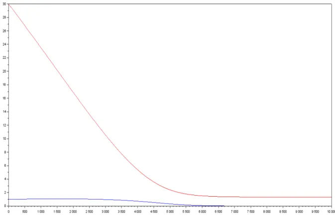
1 concentration of Biomass in blue and Substrate in red in function of time . . . 18 2 gas yield in function of the proportion of species 1 at t=0 in a two species model

with mortality . . . 23 3 population of species 1 in function of time . . . 24 4 population of species 2 in function of time . . . 25

(5)

1 ACKNOWLEDGMENTS

1 Acknowledgments

First of all, I would like to thank M.Rapaport for accepting me in his department UMR MISTEA (Mathematics, Informatics and STatistics for Environment and Agronomy) at INRA Montpellier. I had the good fortune of having him as my advisor and I am grateful for the trust he placed in me, his pedagogical style and his good natured disposition in always being there to answer my queries.

During my two months internship I had the opportunity of observing research environment, I could use my mathematical knowledge to handle a concrete problem and learn LaTeX to write this report.

Without a doubt this was a unique learning experience for me, which I not only enjoyed but which has given me the opportunity to have a better idea of my future professional choices.

(6)

2 INTERNSHIP SEARCH AND CHOICE OF SUBJECT

2 Internship search and choice of subject

I began to actively search for an internship at the end of December, during winter’s vacation. For pecuniary reasons, I wanted to do my internship in my hometown so I sent several internship applications to companies and organisations present in Montpellier (the town is a big pole in agronomy, which is the reason why I got an internship on this field). Since I hadn’t decided yet if I wanted to do research or not, both internships in companies or research institutes were good opportunities for me.

I was glad to have a positive answer for my internship application at MISTEA because, even if the subject isn’t related to econonomics, the mathematical tools were the same, and I know I will eventually use the knowledge I gained during these two months in my studies. Furthermore, the task I was entrusted with seemed to be more challenging than what I could have done in other places.

(7)

3 GENERAL WORKING CONDITIONS

3 General working conditions

My internship was at the Mathematics, Computer Science and Statistics for environment and agronomy (MISTEA) which is an INRA unit located in the Montpellier SupAgro campus.

The working conditions were very good, since I had an office with air conditioning, a personal laptop with running Ubuntu 14.04 and all useful softwares such as matlab,scilab or python. Fur-thermore, a personnal inra email adress was created (for my internship period only) so I could have acess to all the intern exchanges.

(8)

4 REPORT SUMMARY

4 Report summary

My task was to show that , in a batch-type microbiological culture (with no exogenous input or output), a combination of different species can produce more biogas than only one species. We used a system of non-linear differential equations to model the evolution of the critical concentrations (Biogas, Biomass and Substrate). This study has concrete applications in biotechnologies that produce gas responsible of greenhouse effect and the opposite that aim to produce biogas. The topic can also be of great interest for wine producers, since wine is obtained by fermenting grape juice, and the quantity of biogas produced by the bacteria can have a big impact on the final product.

During my internship, I worked on several models, more and more complicated. The idea was to have a better understanding of the subject by beginning with simpler models. Furthermore, results from previous models where sometimes needed, and they also often gave me clues on the behaviour of the other more complex models.

At several times, when I did not had a very clear idea of what was going on or simply when I was stuck, I had resort to computer simulations, on scilab, in order to have some concrete results to think on. I used the Runge-Kutta method of order 2 for the simulations.

During my internship, I used what I had learned in the differential equation course. And, since we did not studied in depth non-linear systems of differential equations, I also learnt a few things, such as the definition of an invariant set.

Key words: Batch bioprocesses, optimisation, Ordinary Differential Equations, invariant set, Scilab, Runge-Kutta method

(9)

5 PRESENTATION OF THE ORGANISATION AND THE INTERNSHIP SUPERVISOR

5 Presentation of the organisation and the internship

super-visor

The "Institut National de Recherche Agronomique" or INRA (in English: National Institute of Research in Agronomy) is a public organisation depending of the ministry of education and research, and the ministry of agriculture. Founded in 1946, the INRA is the first European research organisation on agronomy.It studies questions related to agriculture,environment,territory management and tries to promote sustainable development.

The unit where the internship took place is called Mistea, which stands for "Mathématiques, Informatiques et Statistiques pour l’Environnement et l’Agronomie" (in English: Mathematics, Computer Science and Statistics for Environment and Agronomy). It goal is to achieve statisti-cal studies and advanced mathematistatisti-cal and computer modeling in order to find answers for the questions the INRA is working on.

Alain Rapaport is a French scientist who has been part of INRA since 1997. His knowledgeable research fields are Modelling, dynamical systems, differential equations, control and observation of dynamical systems, optimization and optimal control. He got his PHD in 1994 at "l’École des Mines de Paris". Finally, in 2003, he receives his Habilitation at the University of Montpellier II.

(10)

6 INTRODUCTION

6 Introduction

Here, we are studying the biogas yield of a batch-type microbiological culture: We put together a given quantity of substrate and a given quantity of bacteria (representing the total biomass) and we let them react. The system is closed, which means that there will be no input or output of substrate and biomass whatsoever. Note that in our model, all quantities are measured in term of concentrations. At a given period t, the bacteria will consume an amount of substrate depending on the current concentration of the bacteria, and a function µ of the current concentration of substrate. Then, they produce an amount of biogas depending on the current concentration of the bacteria. The Substrate consumption function, the Biogas yield, the Biomass yield (ie. how much substrate is needed to create a new individual) are factors that depends of the species. Later on, we will add in our model a mortality factor that will also depend of the species.

There are three critical values in our model: Substrate concentration, Biomass concentration and Biogas concentration. The main goal of this internship is studying the existence of overyielding for the biogas production. Overyielding is when a combination of several species have a higher biogas yield than the most productive species, for a given total biomass. Overyielding can also be defined in a more formal way: let n P N the number of species, X P r0, 1sna vector of proportions such that

n

ÿ

i“1

Xi “ 1, λ P Rn` the vector of marginal biogas production of the n species and Λ : λ P R` ÞÑ R`

the asymptotic biogas production function. Then, a definition for overyielding would be: there exist a set Ω ‰ H such that Ω : tX, Λpλ1_{Xq ą max}

i tΛpλiqu.

Four different models will be presented in this report: the model with single species and no mortality, the model with n species and no mortality, the model with single species and mortality and finally, the model with n species and mortality. Each of the four models will be presented following the same pattern. First, we define the model. Then we look for some basic properties for this model (uniqueness of the solution, the interval of the maximal solution. . .), after this we study the asymptotic behaviour of substrate, biomass and biogas and then, we compute the asymptotic biogas production (excepted in the last model where I didn’t had enough time to find the solution. I put the simulations I made instead). Note that for some models, it was needed to reformulate the equations (with a change of variables) to find the asymptotic behaviour of the variables.

(11)

7 THE MODEL WITH SINGLE SPECIES

7 The model with single species

In order to study the existence of overyielding, for a given biomass and substrate quantity at time 0, we need to compare the biogas production of n species with the production of the most efficient species. In order to do that, the first step is to compute an expression for the total gas production in the model with only one species.

Here, we consider the relation between the concentration of substrate S and the concentration of the only bacterium species B, and the production of biogas G. We model this with a two dimension dynamic system. For any t ě 0 :

pCP 1q $ & % 9 Sptq “ ´µpSqBptq Y 9 Bptq “ µpSqBptq Sp0q “ S0 ą 0 Bp0q “ B0 ą 0 and 9 Gptq “ rµpSqBptq Gp0q “ 0 where • t is time.

• Y is the biomass yield factor of the bacterium .

• r is the biogas yield multiplier of the bacterium (ie. how much biogas is produced during a bacterium’s lifespan).

• G(t) is the quantity of biogas produced since t=0. • B(t) is the concentration of biomass at period t. • S(t) is the concentration of substrate at period t.

• µ is the substrate consumption speed of bacterium function, depending on S. It is strictly increasing, locally k-lipschitzian, C2 and µ(0)=0.

• 9Sptq, 9Bptq and 9Gptq represent respectively the consumption of substrate and the production of biomass and biogas at period t.

Note 7.1. Since the equation of G has no influence on the other two equations, we choose to not include it in our system. The asymptotic production of biogas will be considered after having studied the behaviour of the system.

7.1 Physical meaning of the equations

Substrate 9Sptq “ ´µpSqBptq Y

Since we model batch-like bioprocesses, there is no input of substrate. So, S is decreasing at a rate proportional to the consumption of substrate of the bacteria.

Biomass 9Bptq “ µpSqBptq

There is no mortality in this simplified model. So the growth rate of biomass is positive, and increases at a rate proportional to µpSq.

(12)

Gas 9Gptq “ rµpSqBptq

Each unit of biomass created at a period t releases r units of biogas during its lifespan ( 9Gptq “ r 9Bptq). We assume G0 “ 0.

Note 7.2. @t ě 0, let Sptq “ Bptq “ 0 and let t0 ą 0: then @t, 9Sptq “ ´

µpSqBptq

Y “ µpSqBptq “ 9

Bptq “ 0 and Spt0q “ Bpt0q “ 0. So Sptq “ Bptq “ 0 is a solution for the Cauchy problem with

the Spt0q “ 0 or Bpt0q “ 0 initial conditions for all t0 ě 0.

7.2 Basic propositions

Note 7.3. Since µpSq is locally lipschitzian and Y ‰ 0, we can apply Cauchy-Lipschitz theorem (also known as Picard-Lindelöf theorem) so the maximal solution is unique, and every solution is unique on a given interval.

Proposition 7.1. @t ě 0, S(t), B(t) and G(t) are strictly positive. Proof. Substrate Consider (CP1):

Let tαS Ps0; `8r be such that SptαSq ă 0.S is continuous. µ is locally lipschitzian, so there

exist a t0S such that Spt0Sq “ 0. It means that (t, S(t), B(t)) is a solution for the Cauchy

problem associated with the Spt0Sq “ 0 initial condition (for t ě 0). And we saw in Note

2.2 that Bptq “ Sptq “ 0 is a solution for this problem. But Cauchy-Lipschitz also tells us that the solution is unique, so Bptq “ Sptq “ 0 for all t, and since SptαSq ă 0, we have a

contradiction: @t ě 0, Sptq ě 0. Biomass Consider (CP1):

Let tαB Ps0; `8r be such that BptαBq ă 0.B is continuous. µ is locally lipschitzian, so there

exist a t0B such that Spt0Sq “ 0 or Bpt0Bq “ 0. It means that (t, S(t), B(t)) is a solution

for the Cauchy problem associated with the Bpt0Bq “ 0 initial condition (for t ě 0). And we

saw in Note 2.2 that Bptq “ Sptq “ 0 is a solution for this problem. But Cauchy-Lipschitz also tells us that the solution is unique, so Bptq “ Sptq “ 0 for all t, and since BptαBq ă 0,

we have a contradiction: @t ě 0, Bptq ě 0.

Biogas We know 9Gptq “ rµpSqBptq, G0 “ 0, @t Ps0; `8r Sptq ą 0 and Bptq ą 0.Since µ is

strictly increasing, µp0q “ 0, S and B always strictly positive, @t Ps0; `8r µpSq ą 0 ñ 9G “ rµpSqBptq ą 0 ñ Gptq ą 0

Since we don’t want S, B or G to be the null function, @t ě 0, S, B and G are strictly positive.

Corollary 7.1. S is strictly decreasing, and B and G are strictly increasing.

Proposition 7.2. @t ě 0, the interval of t for the maximal solution of a given Cauchy problem is r0; `8r.

Proof. Let tα ă `8 such that the interval of the maximal solution would be r0; tαr. It means at

least one of these three quantities S(t), B(t) or G(t) blows-up in finite time. We will show that this is possible for neither of them:

• For S: S is positive and strictly decreasing, so S is bounded (ie. @t P r0, `8r, Sptq P r0; S0sq

(13)

• For B: let tαě 0 such that lim tÑtα

Bptq “ `8. Then, lim

tÑtα

9

Sptq “ `8 which is in contradiction with the fact that S is C1. So B can not blow-up in finite time.

• For G: let T Ps0; `8r. Using the integral formulation of G, we get:

GpT q “ Gp0q ` T ż 0 9 Gptqdt “ T ż 0 rµpSqBptqdt “ r T ż 0 9 Bptqdt “ rpBpT q ´ B0q

And since B does not blow-up in finite time, this quantity is finite for any T. So G does not blow-up in finite time either.

Proposition 7.3. The asymptotic value of S in `8 is 0.

Proof. Since substrate is strictly decreasing but positive, S admits a limit in `8 we will call lS P r0; `8r.

Let lS ą 0. Then, there is a majorant for 9S, called δ such that δ ą 0:

9

Sptq “ ´µpSqBptq Y ď ´

µplSqB0

Y “ ´δ let T ă t. Using the Mean value inequality, we get:

pSptq ´ SpT qq ď ´δpt ´ T q Sptq ď SpT q ´ δpt ´ T q

but lim

tÑ`8SpT q ` δpt ´ T q “ ´8,so we get limtÑ`8Sptq ď ´8,which is which is in contradiction with

the assumption that lS is strictly positive. So lS “ 0.

Proposition 7.4. The subset of R`, I :“ tt P R`|Y Sptq ` Bptq “ Y S0` B0u is an invariant set

for (CP1).

Proof. Since Y 9Sptq ` 9Bptq “ ´µpSqBptq ` µpSqBptq “ 0 and Y Sp0q ` Bp0q “ Y S0` B0, B(t) and

S(t) are in I for all t in R`.

7.3 Computing the asymptotic biogas concentration:

We have now all the elements needed to compute the asymptotic biogas concentration (ie. lim

tÑ8Gptq). Let T ą 0. Using the integral formulation of G, we get:

GpT q “ Gp0q ` żT 0 rµpSptqqBptqdt GpT q “ r żT 0 µpSptqqBptqdt GpT q “ r żT 0 9 Bptqdt GpT q “ rpBpT q ´ B0q (1)

(14)

And the invariant set gives us the following equality for all t P R`:

Y Sptq ` Bptq “ Y S0` B0

Bptq “ Y pS0´ Sptqq ` B0

(2)

So, combining (1) and (2) we get:

GpT q “ rY pS0´ SpT qq

and using proposition 2.3 we have:

lim

(15)

8 THE MODEL WITH N SPECIES

8 The model with n species

We will now introduce n species in our model instead of just one. Each species has its own biomass and biogas yield multiplier Yi and ri, its own substrate consumption function µi. The

concentration of each species will be noted as Xi while the total biomass will be noted B, as in the

previous model. The new Cauchy problem is, for any t ě 0:

pCP 2q $ ’ & ’ % 9 Sptq “ n ÿ i“1 ´µipSqXiptq Yi @i, 9Xiptq “ µipSqXiptq Sp0q “ S0 ą 0 @i, Xip0q “ X0 ą 0 @t ě 0, n ÿ i“1 Xiptq “ Bptq and 9 Gptq “ n ÿ i“1 riµipSqXiptq Gp0q “ 0

Note 8.1. If Di such that Xip0q “ Bp0q, then (CP2) is equivalent to (CP1).

Note 8.2. @t ě 0, i “ 1, 2 . . . n, let Sptq “ Xiptq “ 0 and t0 ą 0. Then:

9 Sptq “ n ÿ i“1 ´µipSqXiptq Yi “ n ÿ i“1 µipSqXiptq “ 9Bptq “ 0

and Spt0q “ Xipt0q “ 0. So Sptq “ Xiptq “ 0 is a solution for the Cauchy problem associated with

the Spt0q “ 0 or Xipt0q “ 0 initial conditions for all t0 ě 0, i “ 1, 2 . . . n.

8.1 Generalisation of the properties from the previous model

Proposition 8.1. @t ě 0, i “ 1, 2 . . . n, S(t), B(t) and Xiptq are strictly positive.

Proof. Substrate Consider (CP2):

@t ě 0, i P v1, nw, let tαS Ps0; `8r such that SptαSq ă 0.S is continuous. µi is locally

lips-chitzian, so there exist a t0Ssuch that Spt0Sq “ 0. It means that pt, Sptq, X1ptq, X2ptq . . . Xnptqq

is a solution for the Cauchy problem associated with the Spt0Sq “ 0 initial condition (for

t ě 0). And we saw in Note 3.2 that X1ptq “ X2ptq “ . . . Xnptq “ Sptq “ 0 is a solution for

this problem. But Cauchy-Lipschitz also tells us that the solution for this problem is unique, so Xiptq “ Sptq “ 0 for all i and for all t. But since SptαSq ă 0, we have a contradiction:

@t ě 0, Sptq ą 0. Biomass Consider (CP2):

@t ě 0, i P v1, nw, let tα_Xi Ps0; `8r such that Xiptα_Xiq ă 0. Xi is continuous for all i. µi is

locally lipschitzian, so there exist a t0_Xi such that Spt0Sq “ 0 and Xipt0_Xiq “ 0. It means

that pt, Sptq, X1ptq, X2ptq . . . Xnptqq is a solution for the Cauchy problem associated with the

Xipt0_Xiq “ 0 @i P v1, nw, Spt0Sq “ 0 initial condition (for t ě 0). And we saw in Note 3.2 that

X1ptq “ X2ptq “ . . . Xnptq “ Sptq “ 0 is a solution for this problem. But Cauchy-Lipschitz

also tells us that the solution for this problem is unique, so Xiptq “ Sptq “ 0 for all i and for

(16)

8 THE MODEL WITH N SPECIES Biogas @t Ps0; `8r, i “ 1, 2 . . . n, We know 9Gptq “ n ÿ i“1 riµipSqXiptq, G0 “ 0, Sptq ą 0 and Bptq ą

0. Since µ is strictly increasing, µp0q “ 0, S and B always strictly positive, @t Ps0; `8r, i “ 1, 2 . . . n: µpSq, Xiptq ą 0 ñ 9G “

n

ÿ

i“1

riµipSqXiptq ą 0 ñ Gptq ą 0.

Since we don’t want S, G or Xi to be the null function, @t ě 0, i “ 1, 2 . . . n, S, G and Xi

are strictly positive.

Corollary 8.1. S is strictly decreasing, and @i “ 1, 2 . . . n, Xi and G are strictly increasing.

Proposition 8.2. The interval of t for the maximal solution of a given Cauchy problem is r0; `8r. Proof. Let tα ă `8 such that the interval of the maximal solution would be r0; tαr. It means at

least one of these three quantities S(t), B(t) or G(t) blows-up in finite time. We will show that this is possible for neither of them:

• For S: S is positive and strictly decreasing,so S is bounded (ie. @t P r0, `8r, Sptq P r0; S0sq

so S cannot blow-up in finite time. • For B: let tαě 0 such that lim

tÑtα

Bptq “ `8. Then, lim

tÑtα

9

Sptq “ `8 which is in contradiction with the fact that S is C1. So B can not blow-up in finite time.

• For G: let T Ps0; `8r. Using the integral formulation of G, we get:

GpT q “ Gp0q ` T ż 0 9 Gptqdt “ T ż 0 n ÿ i“1 riµipSqXiptqdt ď max i triu T ż 0 n ÿ i“1 µipSqXiptqdt “ max i triu T ż 0 9 Bptqdt “ max i triupBpT q ´ B0q

And since B does not blow-up in finite time, this quantity is finite for any T. So G can not blow-up in finite time either.

Proposition 8.3. The asymptotic value of S in `8 is 0.

Proof. Since substrate is strictly decreasing but positive, S admits a limit in `8 we will call lS P r0; `8r.

(17)

Let lS ą 0. Then, there is a majorant for 9S we will call δ such that δ ă 0:

9 Sptq “ n ÿ i“1 ´µipSqXiptq Yi

ď ´n minitµiplSqu minitXip0qu maxitY u

“ δ

let T ă t. Using the Mean value inequality, we get:

|Sptq ´ SpT q| ď δ|t ´ T | SpT q ď Sptq ` δpt ´ T q

but lim

tÑ`8Sptq ` δpt ´ T q “ ´8,so we get SpT q ď ´8,which is impossible. So lS “ 0.

Proposition 8.4. The subset of R`, I :“ tt P R`|Sptq` n ÿ i“1 Xiptq Yi “ S0` n ÿ i“1 Xip0q Yi u is an invariant set for (CP2). Proof. Since 9Sptq ` n ÿ i“1 9 Xiptq Yi “ ´ n ÿ i“1 ´µipSqXiptq Yi ` n ÿ i“1 µipSqXiptq Yi “ 0 So @i P v1, nw, Xiptq and S(t) are in I for all t in R`.

8.2 Looking for a possibility of overyielding

In this section, we will prove that any combination of species cannot beat the production of the "best" species. This result can be obtain by straight on computation, but we will also show another proof, where we use the invariant set.

Proposition 8.5. For all S0, , Xip0q, Bp0q, there cannot have overyielding for (CP2).

Note 8.3. There is at least one "best" species iOwhose biogas production is higher than all the other

species and its asymptotic biogas production is: lim

T Ñ8Gi0pT q “ maxi triYiuS0 ě riYiS0 “ limT Ñ8GipT q,

(18)

8.2.1 Calculative proof

Proof. We want to show that the asymptotic value of G in 8 is less or equal than the production of the best species. Let T ą 0. Using the integral formulation of G, we get:

GpT q “ Gp0q ` T ż 0 9 Gptqdt “ T ż 0 n ÿ i“1 riµipSqXiptqdt “ n ÿ i“1 ri T ż 0 µipSqXiptqdt “ n ÿ i“1 riYi T ż 0 µipSqXiptq Yi dt ď max i triYiu T ż 0 n ÿ i“1 µipSqXiptq Yi dt “ max i triYiu T ż 0 ´ 9Sptqdt “ max i triYiupS0´ SpT qq

And since lim

tÑ8Sptq “ 0: limT Ñ8maxi triYiupS0´ SpT qq “m axitriYiuS0 “ limT Ñ8GiOpT q

We have lim

(19)

8.2.2 Invariant set proof

Proof. Looking at the invariant set I :“ ! t P R`|Sptq ` n ÿ i“1 Xiptq Yi “ S0` n ÿ i“1 Xip0q Yi ) : @T ě 0: SpT q ` n ÿ i“1 XipT q Yi “ S0` n ÿ i“1 Xip0q Yi n ÿ i“1 Xiptq ´ Xip0q Yi “ S0´ SpT q n ÿ i“1 Xiptq ´ Xip0q YipS0´ SpT qq “ 1 Now, @T ą 0, we compute G(T): GpT q “ Gp0q ` T ż 0 9 Gptqdt “ T ż 0 n ÿ i“1 riµipSqXiptqdt “ n ÿ i“1 ri T ż 0 µipSqXiptqdt “ n ÿ i“1 ri T ż 0 9 Xiptqdt “ n ÿ i“1 ripXipT q ´ Xip0qq “ n ÿ i“1 riYipS0´ SpT qq XipT q ´ Xip0q YipS0´ SpT qq ď max i triYiupS0´ SpT qq n ÿ i“1 XipT q ´ Xip0q YipS0´ SpT qq “ max i triYiupS0´ SpT qq

And since lim

tÑ8Sptq “ 0: limT Ñ8maxi triYiupS0´ SpT qq “ maxi triYiuS0 “ limT Ñ8GiOpT q

We have lim

(20)

9 THE MODEL WITH SINGLE SPECIES MODEL AND MORTALITY

9 The model with single species model and mortality

We now introduce a mortality factor m for bacteria in our model. In order to study its impact on our results, we will start with the one species model. For any t ě 0 :

pCP 3q $ & % 9 Sptq “ ´µpSqBptq Y 9 Bptq “ pµpSq ´ mqBptq Sp0q “ S0 ą 0 Bp0q “ B0 ą 0 and 9 Gptq “ rµpSptqqBptq Gp0q “ 0

As in (CP1), the quantity of biogas produced at a period t depends on the substrate concentra-tion S and the biomass concentraconcentra-tion B at this period. But this time, we subtract the concentraconcentra-tion of dying biomass at period t. So unlike (CP1), the derivative of B may not be positive for all t. In particular, we will see what influence does this have over the limit of S.

9.1 Basic propositions

Proposition 9.1. @t ě 0, S(t), B(t) and G(t) are strictly positive. Corollary 9.1. S is strictly decreasing and G is strictly increasing. Corollary 9.2. S has a limit in `8.

Let lS be this limit.

The proof for Propositions 9.1 and 9.2 are similar to those for, respectively, Propositions 7.1 and 7.2 from section 7.

Note 9.1. With the mortality term, 9Bptq is no longer proportional to 9Sptq, so there is no more invariant set.

Lemma 9.1. Dtα ą 0 such that 9Bptαq ă 0

Proof. @t P r0; `8r:

If we suppose the lemma above to be false, then, for all t, 9B ě 0. We know from proposition 9.1 that µpSq is positive. And since µ is continuous and strictly increasing, µ is a bijective function so for all t, we can define its inverse function µ´1 such that µ´1pµpSqq “ S.

Let S1 and S2 P rSl, S0s such that S1 ą S2. Then, since µ is strictly increasing, µpS1q ą µpS2q.

So S1 ą S2 ô µ´1pµpS1q ą µ´1pµpS2q. And since µpS1q ą µpS2q, µ´1 is an increasing function. So

9

B ě 0 ñ µpSq ě m ñ S ě µ´1pmq ě 0.

On the one hand, we know S is a monotonic C1 function, with a finite limit, which implies that lim

tÑ8

9 Sptq “ 0.

But on the other hand, let lim

tÑ8Bptq “ Bl ď `8. We know Bl ą 0 because B0 ą 0 and we

supposed 9B ě 0. Then: lim tÑ8 9 Sptq “ lim tÑ8´ µpSqBptq Y “ ´ µplSqBl Y ă 0 Which is not possible, so the lemma must be true.

(21)

Corollary 9.3. @t ě tα, 9Bptq ă 0 (from proposition 9.1 and corollary 9.1).

Corollary 9.4. Let Bl be the limit of B in `8: 0 ď Blă `8.

Proposition 9.3. The value of Bl is 0.

Proof. We assume Bl ą 0. Let ´δ “ BptαqpµpSptαqq ´ mq ă 0:

Using corollary 4.3 we have: @t ě tα,

9

Bptq “ BptqpµpSq ´ mq ď ´δ

Let T ă t. Using the Mean value inequality, we get:

pBptq ´ BpT qq ď ´δpt ´ T q Bptq ď BpT q ´ δpt ´ T q

but lim

tÑ`8Bptq´δpt´T q “ ´8,so we get Bptq ď ´8,which is in contradiction with the assumption

that Bl ą 0. So Bl “ 0.

9.2 Reformulating the model

Since S is a monotonic and C1 function on t P r0; `8r, there is a bijection between t and S(t) on this interval. Let Φptq such that:

Φ : t P r0; `8rÞÑ Sptq “ Φptq P rlS; S0s

Then we define Φ´1

pSq as:

Φ´1 _{: Sptq “ Φptq P rl}

S; S0s ÞÑ t P r0; `8r

Lemma 9.2. Let µ a monotonic C1 _{application from U Ă R}n _{to V Ă R and µ}´1 its inverse function. Let u P U and v P V such that µpuq “ v . The derivative of µ´1

pvq is rµ´1s1pvq “ 1 µ1_puq Proof. By definition: µ´1 pµpuqq “ u ñ µ1puqrµ´1s1pvq “ 1 ô rµ´1s1pvq “ 1 µ1_puq

Corollary 9.5. The derivative of Φ´1

pSq is rΦ´1s1pSq “ ´ Y

µpSqBpΦ´1_pSqq, @t ě 0.

Proposition 9.4. An alternative formulation for (CP3) is:

pCP 3q : dB dS “ Y ˆ m µpSq ´ 1 ˙ BpS0q “ B0 ą 0

(22)

Proof. We do a change of variable, by replacing t by Φ´1pSq. It permits us to get rid of the S equation. Concerning B, using Corollary 9.5 we can say:

9 Bptq “ 9BpΦ´1 pSqq “ rΦ´1s1pSq 9BpΦ´1pSqq “ ´Y BpΦ ´1 pSqqpµpSq ´ mq µpSqBpΦ´1_pSqq “ ´Y ` Y m µpSq “ Y ˆ m µpSq ´ 1 ˙

Corollary 9.6. Using Proposition 9.3: BplSq “ 0

9.3 The asymptotic value of S

One’s first guess would be that the limit of S is still 0, but the figure below seems to tell us the opposite. We will show in this section that this assumption is untrue.

(23)

Note 9.2. The Runge-Kutta method of order 2 has been used for all the simulations in this report. Theorem 9.1. The limit of S cannot be 0

Proof. µ is k-lipschitz, which means that Dk P R such that @x, y P R`˚, |µpxq ´ µpyq| ď k|x ´ y|

so:

@S Ps0; S0s, |µpSq ´ µp0q| ď k|S ´ 0|

ô µpSq ď kS (4)

Let’s suppose lS “ 0. Using the integral formulation of B(S), we get:

BpS0q “ BplSq ` żS0 lS dB dSpSqdS “ żS0 0 Y p m µpSq´ 1qdS “ żS0 0 Y m µpSqdS ´ Y S0 And, according to (4), we have :

żS0 0 Y m µpSqdS ´ Y S0 ě żS0 0 Y m kS dS ô żS0 0 Y m µpSqdS ´ Y S0 ě Y m k żS0 0 1 SdS And Y m k żS0 0 1

SdS diverges in 0 so there is a contradiction: lS ‰ 0.

9.4 The asymptotic value of G

Proposition 9.5. The value of the biogas production for a given substrate concentration is: @S PsSl; S0s, dG dSpSq “ ´rY Proof. 9 Gptq “ 9GpΦ´1 pSqq “ rΦ´1pSqs1GpΦ9 ´1 pSqq “ ´Y rµpSqBpΦ ´1 pSq µpSqBpΦ´1_pSqq “ ´rY

We can now compute the asymptotic value of G, using the integral formulation of G(S):

GpS0q “ GpSlq ` żS0 Sl dG dSpSqdS ô GpSlq ´ żS0 Sl rY dS ô GpSlq “ żS0 Sl rY dS ô GpSlq “ rY pS0´ Slq

The asymptotic production of biogas is GpSlq “ rY pS0´ Slq and is decreasing with respect to

(24)

10 THE MODEL WITH N SPECIES AND MORTALITY

10 The model with n species and mortality

In this model, every species has its own mortality term mi. We will first list the propositions

from the previous model with single species and mortality that stay true. Then, using scilab simulations, we will explain how overyielding is indeed possible in a model with mortality.

pCP 4q $ ’ & ’ % 9 Sptq “ n ÿ i“1 ´µipSqXiptq Yi @i, 9Xiptq “ XiptqpµipSq ´ miq Sp0q “ S0 ą 0 @i, Xip0q “ X0 ą 0 @t ě 0, n ÿ i“1 Xiptq “ Bptq and 9 Gptq “ n ÿ i“1 riµipSqXiptq Gp0q “ 0

10.1 Generalisation of the properties from the previous models

Proposition 10.1. @t ě 0, i P v1, nw, S, G and Xi are strictly positive.

Corollary 10.1. S is strictly decreasing and G is strictly increasing.

Corollary 10.2. Since S is strictly positive and strictly decreasing, S has a limit noted lS.

The proof for Propositions 10.1 and 10.2 are similar to those for Propositions 8.1 and 8.2 from section 8.

Note 10.1. Here again, 9Bptq and 9Sptq are not proportional, so there is no invariant set. Lemma 10.1. Dtαą 0 such that 9Bptαq ă 0

Proof. @t P r0; `8r:

If we suppose the lemma above to be false, then, for all t positive, 9Bptq ě 0. We know from proposition 10.1 that µpSq is positive. So 9Bptq ě 0 ñ µpSq ě m. And since µ is continuous and strictly increasing, µ is a bijective function so for all t, we can define µ´1

pSq such that µpµ´1

pSqq “ S and S ě µ´1pmq ě 0 for all t ě 0.

On the one hand, we know S is a monotonous C1 function, with a finite limit, which implies that lim

tÑ8

9

Sptq “ 0.

But on the other hand, let lim

tÑ8Bptq “ Bl ď `8. We know Bl ě 0 because B0 ą 0 and we

supposed 9Bptq ě 0. Then: lim tÑ8 9 Sptq “ lim tÑ8´ µpSqBptq Y “ ´ µplSqBl Y ă 0 We have reached a contradiction, so the lemma is true.

(25)

Corollary 10.3. @t ě tα, 9Bptq ă 0 (from proposition 10.1 and Corollary 10.1)

Proposition 10.3. The asymptotic value of B in `8 called Bl is 0.

Proof. We assume Bl ą 0. Let ´δ “ B0pµpSptαqq ´ mq ă 0:

9

Bptq “ BptqpµpSq ´ mq ď ´δ Let T ă t. Using the Mean value inequality, we get:

pBptq ´ BpT qq ď ´δpt ´ T q Bptq ď BpT q ´ δpt ´ T q

but lim

tÑ`8BpT q ` δpt ´ T q “ ´8,so we get Blď ´8,which is in contradiction with the assumption

we have made. So Bl“ 0.

10.2 Reformulating the model

Proposition 10.4. An alternative formulation for (CP4) is: @S P rlS, S0s,

pCP 4q $ & % dXi dS pSq “ XipΦ´1pSqqpµipSq ´ miq ´ řn j“1XjpΦ´1pSqqµjpSq Yj BpS0q “ B0 ą 0 @t ě 0, n ÿ i“1 Xiptq “ Bptq

Proof. We do a change of variable, by Φ´1

pSq. It permits us to get rid of the S equation. We use Corollary 4.5 to compute rΦ´1 pSqs1: 9 Xiptq “ 9XipΦ´1pSqq “ rΦ´1s1pSq 9XipΦ´1pSqq “ XipΦ ´1 pSqqpµipSq ´ miq ´ řn j“1XjpΦ´1pSqqµjpSq Yj

Corollary 10.4. 9B can be also written as: @S P rlS; S0s,

dB dSpSq “ n ÿ i“1 XipΦ´1pSqqpµipSq ´ miq ´ řn j“1XjpΦ´1pSqqµjpSq Yj

Corollary 10.5. Since the asymptotic value of B in `8 is 0 (cf. Proposition 10.3), @i P v1, nw XiplSq “ 0.

10.3 The asymptotic value of S

In this section, we are going to prove that as in the previous model, The asymptotic value of S cannot be 0.

(26)

Proof. @i P v1, nw, µi is ki-lipschitz, which means that Dki P R such that @x, y P R˚`,

|µipxq ´ µipyq| ď ki|x ´ y| for every i. So:

@S Ps0; S0s, |µipSq ´ µip0q| ď ki|S ´ 0|

ô µipSq ď kiS

(5)

Let’s suppose lS “ 0. Using the integral formulation of B(S), we get:

BpS0q “ BplSq ` żS0 lS dB dSpSqdS “ żS0 0 dB dSpSqdS “ żS0 0 n ÿ i“1 XipΦ´1pSqqpµipSq ´ miq ´ řn j“1XjpΦ´1pSqqµjpSq Yj dS “ żS0 0 n ÿ i“1 XipΦ´1pSqqp´µipSq ` miq řn j“1XjpΦ´1pSqqµjpSq Yj dS ě min j tYju żS0 0 n ÿ i“1 XipΦ´1pSqqp´µipSq ` miq řn j“1XjpΦ´1pSqqµjpSq dS ě min j tYju ˜ żS0 0 n ÿ i“1 ´XipΦ´1pSqqµipSq řn j“1XjpΦ´1pSqqµjpSq dS ` min i tmiu żS0 0 n ÿ i“1 XipΦ´1pSqqq řn j“1XjpΦ´1pSqqµjpSq dS ¸

And, according to (5), we have :

min j tYju ˜ żS0 0 n ÿ i“1 ´XipΦ´1pSqqµipSq řn j“1XjpΦ´1pSqqµjpSq dS ` min i tmiu żS0 0 n ÿ i“1 XipΦ´1pSqqmi řn j“1XjpΦ´1pSqqµjpSq dS ¸ ě min j tYju ˜ żS0 0 n ÿ i“1 ´XipΦ´1pSqqµipSq řn j“1XjpΦ´1pSqqµjpSq dS ` min i tmiu żS0 0 n ÿ i“1 XipΦ´1pSqq řn j“1XjpΦ´1pSqqkjS dS ¸ ě min j tYju ˜ żS0 0 n ÿ i“1 ´XipΦ´1pSqqµipSq řn j“1XjpΦ´1pSqqµjpSq dS ` minitmiu maxjtkju żS0 0 n ÿ i“1 XipΦ´1pSqq řn j“1XjpΦ´1pSqqS dS ¸ “ min j tYju ˜ żS0 0 n ÿ i“1 ´XipΦ´1pSqqµipSq řn j“1XjpΦ´1pSqqµjpSq dS ` minitmiu maxjtkju żS0 0 1 SdS ¸ And minitmiu maxjtkju żS0 0 1

(27)

10.4 About overyielding

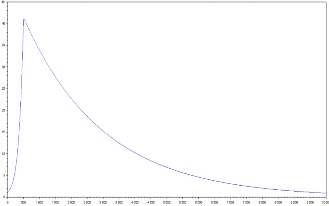
I wasn’t able to mathematically prove the existence of overyielding in the last model. However, I did some simulations on scilab to show it existence, and give us clues to explain overyielding. We run a simulation on a two species model, where species one has a much higher mortality and biogas yield multiplier.

Figure 2: gas yield in function of the proportion of species 1 at t=0 in a two species model with mortality

Since this is a two species model, we can deduce the proportion of species two from the propor-tion of species 1. And we can see on the graphic that the maximum of this funcpropor-tion is not reached in 0 or 1. So there are some proportions for species 1 and 2 where there is overyielding. In fact, the optimal proportion seems to be a very high proportion of pecies one, but different from 0.

(28)

Now let us compare the behaviour of the biomass population in the "extreme" cases (where the proportion of species 1 at period 0 p1p0q is equal to 0 or 1).

First, the case where p1p0q “ 1:

(29)

And then the case where p1p0q “ 0:

Figure 4: population of species 2 in function of time

Species one has a greater density at the beginning, but it declines much more rapidly than species 2 because of the higher mortality rate. To have overyielding in this model, we put a high proportion of species one to have a good yield at the beginning, and since this species has a high mortality rate, it population will die quickly, leaving enough room for the population of species 2 to grow, which will allow us to maintain our yield later on and thus do better than the cases where there is only one species.

By using the properties of each species, in some cases, we can make a combination that would have the most optimal yield at any point of time. However, we can make the assumption that if a species had the highest biogas yield (ie. riYi) and the lowest mortality rate, then no combination

(30)

11 CONCLUSION

11 Conclusion

We managed to show that, in a model without mortality, there cannot have overyielding. So, adding a mortality term is crucial since strong evidence suggest that overyielding would be possible in this scenario.

During this internship, I learned a lot on the approach for solving problems in applied mathe-matics: in particular, I discovered the crucial role of computer simulation which is a very useful support, allowing us to validate or invalidate our intuitions, or giving us a lead when we are stuck. I also familiarised myself with the world of research. For example, I learned a few things about the attribution of funds for PHD students, see what the daily life looks like. . . This internship was intellectually rewarding for me and also permitted me to refine my professional project.

(31)

REFERENCES

References

[1] UMR MISTEA http://www6.montpellier.inra.fr/mistea/Presentation. [2] INRA http://institut.inra.fr/Missions.

[3] Analyse numérique et équations différentielles J-P. Demailly, 1991.

Optimisation and study of batch bioprocesses dynamics

HAL Id: hal-02799113

https://hal.inrae.fr/hal-02799113

Optimisation and study of batch bioprocesses dynamics

Luke Lo Seen

To cite this version:

Internship Report:

Optimisation and study of batch bioprocesses

dynamics

Lo Seen Luke

L3 Économie et Mathématiques

Toulouse 1 Capitole

Mathématiques, Informatique et Statistiques pour l’Environnement et l’Agronomie

(MISTEA) from Institut National de Recherche Agronomique (INRA),

Montpellier, France

Contents

List of Figures

1

Acknowledgments

2

Internship search and choice of subject

3

General working conditions

4

Report summary

5

Presentation of the organisation and the internship

super-visor

6

Introduction

7

The model with single species

7.1

Physical meaning of the equations

7.2

Basic propositions

7.3

Computing the asymptotic biogas concentration:

8

The model with n species

8.1

Generalisation of the properties from the previous model

8.2

Looking for a possibility of overyielding

9

The model with single species model and mortality

9.1

Basic propositions

9.2

Reformulating the model

9.3

The asymptotic value of S

9.4

The asymptotic value of G

10

The model with n species and mortality

10.1

Generalisation of the properties from the previous models

10.2

Reformulating the model

10.3

The asymptotic value of S

10.4

About overyielding

11

Conclusion

References