HAL Id: tel-03198757
https://tel.archives-ouvertes.fr/tel-03198757
Submitted on 15 Apr 2021HAL is a multi-disciplinary open access
archive for the deposit and dissemination of sci-entific research documents, whether they are pub-lished or not. The documents may come from teaching and research institutions in France or abroad, or from public or private research centers.
L’archive ouverte pluridisciplinaire HAL, est destinée au dépôt et à la diffusion de documents scientifiques de niveau recherche, publiés ou non, émanant des établissements d’enseignement et de recherche français ou étrangers, des laboratoires publics ou privés.
analysis and modeling of multi-wavelength flares and
preparation of CTA
Anton Dmytriiev
To cite this version:
Anton Dmytriiev. Exploring active galactic nuclei at extreme energies : analysis and modeling of multi-wavelength flares and preparation of CTA. Earth Sciences. Université de Paris, 2020. English. �NNT : 2020UNIP7052�. �tel-03198757�
Observatoire de Paris
Laboratoire Univers et Th´eories (LUTH)
Exploring Active Galactic Nuclei at
extreme energies: analysis and modeling
of multi-wavelength flares and preparation
of CTA
par
Anton Dmytriiev
Th`
ese de doctorat en astronomie et astrophysique
Dirig´ee par H´el`ene SOL et par Andreas ZECH
Pr´esent´ee et soutenue publiquement le 27 novembre 2020 devant un jury compos´e de:
St´ephane CORBEL, Professeur, Universit´e de Paris, Pr´esident
Paula CHADWICK, Professeur, Universit´e de Durham (Royaume-Uni), Rapporteur Gilles HENRI, Professeur, Universit´e Grenoble Alpes, Rapporteur
Markus B ¨OTTCHER, Professeur, Universit´e du Nord-Ouest (Afrique du Sud), Examinateur
Bohdan HNATYK, Professeur, Universit´e nationale Taras-Chevtchenko de Kiev (Ukraine), Examinateur
H´el`ene SOL, Professeur, Observatoire de Paris, Directrice de th`ese
Titre: Exploration des Noyaux Actifs de Galaxies aux ´energies extrˆemes: analyse et mod´elisation des sursauts multi-longueurs d’onde et pr´eparation du CTA
R´esum´e: De nombreuses questions li´ees `a la physique des jets des Noyaux Actifs de Galaxies restent ouvertes. Une classe particuli`ere d’AGN, les blazars, a un jet pointant vers la Terre. Une telle orientation du jet nous permet de sonder une riche vari´et´e de ph´enom`enes physiques mal compris sur les ´ecoulements relativistes. Les blazars montrent une ´emission non thermique, provenant du jet, qui est tr`es variable sur tout le spectre ´electromagn´etique, des radiofr´equences aux rayons gamma du TeV. Le flux d’´energie peut augmenter d’un ordre de grandeur sur des ´echelles de temps aussi courtes que quelques minutes, un ph´enom`ene appel´e “sursaut” (flare), et aussi longues que des mois ou mˆeme des ann´ees. Malgr´e la quantit´e croissante de donn´ees disponibles sur plusieurs longueurs d’onde (multi-wavelength, MWL), l’origine et les m´ecanismes physiques derri`ere les sursauts fr´equemment observ´es dans les blazars ne sont toujours pas bien compris. De nombreuses tentatives ont ´et´e faites pour d´ecrire les flares avec diff´erents mod`eles d’´emission, mais les propri´et´es d´etaill´ees de l’´evolution temporelle des flux dans diff´erentes bandes spectrales restent difficiles `a reproduire. Afin d’identifier les processus physiques impliqu´es lors des sursauts de blazars, j’ai d´evelopp´e un code radiatif polyvalent, bas´e sur un traitement d´ependant du temps de l’acc´el´eration des particules, de l’´echappement et du refroidissement radiatif. Le code calcule l’´evolution dans le temps de la fonction de distribution des ´
electrons dans la zone d’´emission du blazar et le spectre de l’´emission Synchrotron Self-Compton (SSC) par ces ´electrons. J’ai appliqu´e le code `a un sursaut multi-lambda g´eant du blazar Mrk 421, repr´esentant de la classe des BL Lacertae, qui est le sursaut le plus brillant d´etect´e jusqu’ici en provenance de cette source. Dans notre approche, nous consid´erons le sursaut comme une perturbation mod´er´ee de l’´etat de flux stationnaire et recherchons des interpr´etations avec un nombre minimum de param`etres libres. En cons´equence, j’ai d´evelopp´e un nouveau sc´enario physique de l’activit´e observ´e pendant le sursaut, qui d´ecrit l’ensemble des donn´ees, comprenant des spectres `a l’´etat haut de la source dans diff´erentes gammes d’´energie, et des courbes de lumi`ere multi-lambda du domaine optique aux rayons gamma VHE. Dans ce sc´enario, le processus d´eclenchant le sursaut est l’acc´el´eration des particules par un processus de type Fermi du second ordre, dˆu `a la turbulence qui emerge au voisinage de la r´egion d’´emission stationnaire du blazar.
Enfin, j’ai contribu´e `a la pr´eparation du Cherenkov Telescope Array (CTA), qui est un observatoire de rayons gamma au sol de nouvelle g´en´eration, dont l’entr´ee en service est pr´evue `a partir de 2022. L’instrument, qui est actuellement en cours de d´eveloppement, aura des performances consid´erablement am´elior´ees par rapport aux Imaging Atmospheric Cherenkov Telescopes (IACTs) qui sont actuellement en fonc-tionnement, y compris une couverture spectrale sans pr´ec´edent de quelques dizaines de GeV `a ∼300 TeV. Dans le cadre du CTA, j’ai effectu´e des simulations de perfor-mances optiques du Gamma-Ray Cherenkov Telescope (GCT), l’un des trois mod`eles propos´es de t´elescopes de petite taille (SST) pour CTA. De plus, en utilisant les ob-servations d’´etoiles brillantes effectu´ees par le prototype de t´elescope install´e sur le site de l’Observatoire de Paris `a Meudon, j’ai ´etudi´e l’effet de la micro-rugosit´e des miroirs du t´elescope sur la fonction d’´etalement du point (PSF) et calcul´e le niveau de qualit´e de polissage des miroirs requis pour optimiser les performances.
Mots clefs: Noyaux Actifs de Galaxies ; Cherenkov Telescope Array ; sursauts des blazars ; mod´elisation d’´emission ; acc´el´eration des particules ; performances optiques ; analyse des donn´ees de rayons gamma ; High Energy Stereoscopic System; Mrk 421 ; 3C 279
Abstract: Many questions related to the physics of jets of Active Galactic Nu-clei remain open. A particular subclass of AGN, blazars, have a jet pointing towards the Earth. Such suitable orientation of the jet allows us to probe a rich variety of poorly understood physical phenomena related to relativistic outflows. Blazars show non-thermal emission, originating from the jet, which is highly variable across the entire electromagnetic spectrum, from radio frequencies to TeV γ-rays. The energy flux can enhance by an order of magnitude on time-scales as short as minutes, a phe-nomenon referred to as a “flare”, and as long as months or even years. Despite the growing amount of available multi-wavelength (MWL) data, the origin and the phys-ical mechanisms behind the frequently observed flaring events in blazars are still not well understood. Many attempts have been made to describe the flares with different emission models, but detailed properties of flux variation patterns (light curves) in dif-ferent wavebands remain difficult to reproduce. In order to identify physical processes that are involved during blazar outbursts, I have developed a versatile radiative code, based on a time-dependent treatment of particle acceleration, escape and radiative cooling. The code computes time evolution of the distribution function of electrons in the blazar emitting zone and the spectrum of the Synchrotron Self-Compton (SSC) emission by these electrons. I applied the code to a giant MWL flare of the blazar Mrk 421, a representative of the BL Lacertae class, which is the brightest VHE flare ever detected from this source. In our approach, we consider the flare as a moderate perturbation of the quiescent state and search for interpretations with a minimum number of free parameters. As a result, I developed a novel physical scenario of the flaring activity that describes the data set, comprising spectra in the high state of the source in different energy ranges, and MWL light curves from the optical domain to the VHE γ-ray band. In this scenario, the process initiating the outburst is the second-order Fermi acceleration of particles due to turbulence arising in the vicinity of the blazar stationary emission region.
In this thesis, I also performed analysis of High Energy Stereoscopic System (H.E.S.S.) data of two giant flares of the blazar 3C 279, a representative of the Flat Spectrum Radio Quasars (FSRQ) class.
Finally, I contributed to preparation of Cherenkov Telescope Array (CTA), which is a new-generation ground-based γ-ray observatory, expected to start operations in 2022. The instrument, which is presently under development, will have greatly im-proved performance compared to currently operating Imaging Atmospheric Cherenkov Telescopes (IACTs), including unprecedented spectral coverage from a few tens of
posed designs of Small-Size Telescopes (SST) for CTA. Also, using the observations of bright stars done by the telescope prototype installed on the site of Paris Observatory in Meudon, I studied the effect of micro-roughness of the telescope mirrors on the point spread function (PSF) and calculated the level of the mirror polishing quality required to optimize the performances.
Keywords: Active Galactic Nuclei ; Cherenkov Telescope Array ; blazar flares ; emission modeling ; acceleration of particles ; optical performance ; gamma-ray data analysis ; High Energy Stereoscopic System ; Mrk 421 ; 3C 279
Abstract iii
List of Figures xii
List of Tables xxvii
Acronyms xxviii
Acknowledgments xxxi
Dedication xxxiii
1 Introduction 1
2 Active Galactic Nuclei 5
2.1 The AGN zoo . . . 6
2.2 Unified scheme of AGN phenomenon . . . 10
2.2.1 What defines the observed luminosity? . . . 12
2.2.2 Radio-loud or radio-quiet? . . . 14
2.2.3 Orientation effects . . . 17
2.3 AGN jets . . . 19
2.3.1 Imaging of jets . . . 19
2.3.3 High-energy particles in jets . . . 22
2.3.4 Energy dissipation . . . 23
2.3.5 Relativistic motions in jets . . . 24
2.4 Blazars . . . 26
2.4.1 Doppler boosting . . . 26
2.4.2 Blazar emission . . . 28
2.4.3 Blazar sequence . . . 30
2.4.4 Probing the Universe with blazars . . . 32
3 Cherenkov gamma-ray astronomy and H.E.S.S. data analysis 33 3.1 VHE gamma-ray astronomy . . . 35
3.1.1 Detection of VHE gamma-rays with an IACT . . . 35
3.1.2 Presently operating IACTs . . . 43
3.2 H.E.S.S. experiment . . . 45
3.2.1 Overview . . . 45
3.2.2 The optical system . . . 46
3.2.3 The cameras . . . 46
3.2.4 The trigger system . . . 48
3.2.5 Data analysis and reconstruction . . . 48
3.3 Analysis of H.E.S.S. data of 3C 279 flare . . . 52
3.3.1 The studied source: 3C 279 . . . 52
3.3.2 VHE flares of 3C 279 detected by H.E.S.S. in 2018 . . . 53
3.3.3 Analysis of H.E.S.S. 3C 279 data : January 2018 flare . . . 55
3.3.4 Analysis of H.E.S.S. 3C 279 data : June 2018 flare . . . 56
3.4 Discussion and perspective . . . 60
4 Modeling of AGN emission: stationary models 63 4.1 Origin of blazar broad-band emission . . . 64
4.1.1 Leptonic (SSC and EC) and hadronic models . . . 64
4.1.2 Blob-in-jet model . . . 67
4.1.3 Synchrotron emission . . . 70
4.1.4 Inverse Compton emission . . . 72
4.1.5 Gamma-gamma pair production . . . 74
4.1.6 Transformation to observer’s frame . . . 75
4.2 EBL absorption . . . 76
5 Modeling of AGN emission: time-dependent approach 79 5.1 General approach and the kinetic equation . . . 80
5.1.1 Particle injection . . . 81
5.1.2 Particle radiative cooling . . . 82
5.1.3 Particle acceleration . . . 83 5.1.4 Particle escape . . . 104 5.2 EMBLEM code . . . 105 5.2.1 Numerical implementation . . . 106 5.2.2 Input parameters . . . 115 5.2.3 Code architecture . . . 118
5.2.4 Examples of simulated flares . . . 119
5.3 Physical modeling of AGN flares . . . 123
5.3.1 What causes the observed variability in the VHE γ-ray regime ? 123 5.3.2 One-zone models . . . 125
5.3.3 Multiple-zone models . . . 126
6 Modeling of a MWL flare of Mrk 421 129 6.1 The studied source: Mrk 421 . . . 131
6.2 Modeling of the low state of the source . . . 133
6.2.2 Mrk 421 low-state emission: physical modeling and discussion 135
6.3 Observational data set of the February 2010 flare of Mrk 421 . . . 143
6.3.1 Archival data . . . 143
6.3.2 Analysis of Fermi-LAT gamma-ray data . . . 146
6.4 A general criterion to test one-zone flaring scenario with a passing shock wave . . . 149
6.5 Physical modeling of Mrk 421 February 2010 flare . . . 158
6.5.1 One-zone model . . . 159
6.5.2 Two-zone model . . . 163
6.6 Discussion and perspective . . . 181
7 Preparation of Cherenkov Telescope Array 191 7.1 CTA project . . . 191
7.1.1 Overview . . . 191
7.1.2 Future science with CTA . . . 194
7.2 Gamma-Ray Cherenkov Telescope: overview and prototyping . . . 199
7.2.1 Overview . . . 199
7.2.2 Prototyping . . . 201
7.3 Gamma-Ray Cherenkov Telescope: performance . . . 202
7.3.1 Ideal optical performance . . . 204
7.3.2 Non-ideal optical performance . . . 209
7.3.3 Modeling of the PSF of the pGCT . . . 213
7.4 Discussion and perspective . . . 221
8 Conclusion and perspective 223
Appendices 227
shock perturbing a steady-state electron spectrum 229 A.1 Assumptions and boundary conditions . . . 229 A.2 Solving by characteristics . . . 231 A.3 Final solution . . . 233
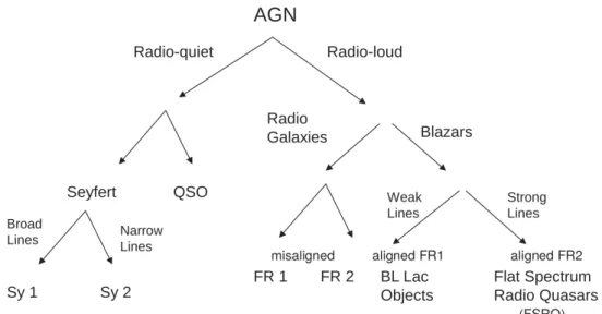
2.1 Observational classification of AGN. The division is based on the prop-erties, such as the level of radio flux and presence of optical lines in the spectra. (adapted from Dermer & Giebels (2016)) . . . 7
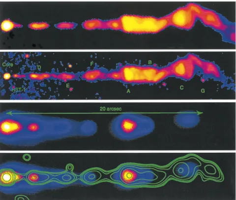
2.2 Illustration of the difference between morphology of the radio emission of FR I and FR II galaxies. Top: a radio image of an example FR I radio galaxy M87, on different spatial scales from the outer radio lobes to the jet launching region in the vicinity of the black hole. One can see that the core region dominates the observed radio emission. (Credit: NRAO, 90 and 20 cm VLA, 20 cm and 7 mm VLBA, and 3mm global VLBI ; image source: Blandford et al. (2019)). Bottom: radio image of an example FR II galaxy Cygnus A. One can see the jets emanating from the core region, which after a certain distance dissipate into gi-ant radio lobes featuring conspicuous hot-spots at their extreme ends. (Credit: NSF/NRAO/AUI/VLA ; image source: chandra.harvard.edu) 9
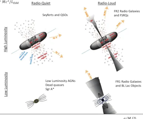
2.3 Illustration of a typical unification scenario for the AGN phenomenon. In this model, the activity of a galactic nucleus is controlled by only two parameters: mass-accretion rate regulating the luminosity of the source, and the central black hole spin responsible (supposedly) for a presence of a jet and therefore prominent radio emission. Finally, orientation of the observer’s line of sight with respect to the symmetry axis defines the observational properties such as width of emission lines in spectra, and observational appearance of radio-loud AGN, as well as the intensity of their γ-ray emission. Blazars, comprising BL Lacs and FSRQs, are FR I and FR II galaxies respectively with the jet aligned with the line of sight. (adapted from Dermer & Giebels (2016)) . . . 11
2.4 Illustration of the jet launching process. Top: schematic representa-tion of the Blandford & Znajek (1977) and Blandford & Payne (1982) mechanisms. The jet is driven by magnetic field lines twisted by the black hole frame-dragging and/or the differentially rotating accretion disk. The jet is attached via magnetic field lines to the BH event horizon and to the accretion disk and pumps out their rotational en-ergy (Credit: NASA, ESA, and A. Feild (STScI)). Bottom: example of general-relativistic magnetohydrodynamic simulations of jet launch-ing. The left panel displays transverse slices of the logarithm of medium density, the right panel – same for the logarithm of the proper velocity of the medium γv. As one can see, the magnetic field lines (indicated in black) that are connected to the event horizon, are responsible for the Poynting flux dominated jet launching, while those connected to the accretion disk drive a matter-dominated outflow. (adapted from Liska (2019)) . . . 16
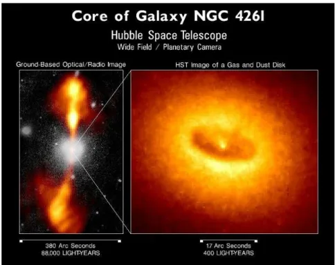
2.5 The active galactic nucleus NGC 4261. Left : superposition of images in the optical and radio band, showing the central core and a pair of relativistic jets emanating from it. Right : a zoom into the central region, showing obscuring dusty torus. (Credit: HST/NASA/ESA, adapted from Jaffe et al. (1993)) . . . 18
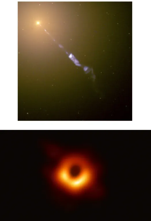
2.6 Top: high-resolution image of the M87 jet obtained by Hubble Space Telescope (Credit: NASA). Bottom: image of the shadow of the M87 black hole (Credit: EHT collaboration ; image source: eventhorizonte-lescope.org). . . 21
2.7 Multi-band view of the jet of M87. Top panel : VLA image at 14.435 GHz. Second panel : optical image (in the red part of the optical spectrum) obtained by Hubble Space Telescope. Third panel : Chandra X-ray Observatory image. Fourth panel : same as third panel, but with superimposed contours of smoothed optical image. The brightness level is displayed with a logarithmic scale for radio and optical images, and with linear scaling for the X-ray image. (adapted from Marshall et al. (2002)) . . . 23
2.8 Illustration of apparent superluminal motions in relativistic jets. Top: Observations of superluminal motion of two knots (top and bottom panel) in PKS 1510-089 (z=0.361) performed in radio band by VLBA at 43 GHz. Contours display the intensity level of the total flux, and the color – of the polarized flux. White linear segments indicate the direction of the linear polarization. The first knot has an apparent velocity of 24 ± 2 c, and the second one of 21.6 ± 0.6 c. The scale of the y-axis is 0.5 pc / 0.1 mas. (adapted from Marscher et al. (2010)). Bot-tom: a scheme explaining the origin of apparent superluminal motions. (adapted from Courvoisier (2013)) . . . 25
2.9 An example of blazar SED. Black points indicate MWL data set (host galaxy subtracted) of HBL BL Lac object Mrk 421 (analyzed in this thesis). Green and red curves represent the SSC models assuming a different variability time-scale. (adapted from Abdo et al. (2011)) . . 29
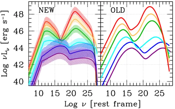
2.10 Updated (left ) and original (right ) blazar sequence. The initial clas-sification was performed based on the radio flux, while the revised version uses γ-ray flux. The curves display SEDs of blazars, with color sequence from red to violet corresponding to the sequence FSRQ – LBL – IBL – HBL. (adapted from Ghisellini et al. (2017)) . . . 31
3.1 Feynman diagram of the Bethe-Heitler pair production process (left ), and of the Bremsstrahlung process (right ). . . 36
3.2 A schematic representation of an electromagnetic (left ) and a hadronic (right ) air shower. (adapted from Wagner (2006)) . . . 37
3.3 Computer simulation of a γ-ray-induced (left ) and a hadron-induced (right ) air shower. (adapted from V¨olk & Bernl¨ohr (2009)) . . . 38
3.4 Huygens’ construction for the wavefront of Cherenkov emission by a relativistic charged particle moving through a medium at a constant velocity exceeding the speed of light in this medium (adapted from Longair (2011)) . . . 39
3.5 Illustration of the IACT observational technique. A VHE γ-ray enters the Earth atmosphere and initiates an electromagnetic cascade. Ul-trarelativistic particles of the cascade emit Cherenkov light, which is detected by ground-based telescope(s). (image source: isdc.unige.ch) . 41
3.6 Difference between Cherenkov images of events caused by particles of different types (γ-ray, hadron and muon) seen by an IACT camera. Left panel : Cherenkov images of γ-ray-induced (left) and hadron-induced (right) air showers. One can see that the γ-ray events have an elliptical-like shape, whereas hadronic events display irregular and inhomoge-neous morphology with multiple islands. Right panel : Cherenkov im-ages of muon events for a muon hitting the telescope mirror and pro-ducing a ring image (left) and hitting the ground close to the periphery and producing an arc image (right). (adapted from V¨olk & Bernl¨ohr (2009)) . . . 42
3.7 Top: VERITAS array in Arizona, USA. Bottom: MAGIC system on Canary Islands in Spain. (Credits: MAGIC and VERITAS collabora-tions) . . . 44
3.8 The full H.E.S.S. array in Namibia. (Credit: H.E.S.S. Collaboration, Frikkie van Greunen) . . . 45
3.9 Different H.E.S.S. telescopes. Top: A close view of the 12-meter diam-eter H.E.S.S. telescopes (CT1-4) seen from different angles, showing the mechanical structure (left), and the segmented telescope mirror (right). Photographs taken during July 2018 shift on the H.E.S.S. site (A. Dmytriiev, 2018). Bottom: A close view of the large 28-meter H.E.S.S. telescope (CT5) (Credit: H.E.S.S. Collaboration, Frikkie van Greunen) . . . 47
3.10 Event reconstruction in Hillas analysis. Top: scheme representing the Hillas parametrization (adapted from Garrigoux (2015)). Bottom: im-ages of an air shower seen by four different telescopes (left) and geo-metric reconstruction of the true source position in the stereo-vision observational mode (right) (adapted from De Naurois (2012)) . . . . 50
3.11 Illustration of three periods of H.E.S.S. follow-up observations of 3C 279 in 2018 after an alert from Fermi -LAT. Blue and green points in the top part of the figure indicate Fermi -LAT γ-ray photon flux of 3C 279 above 100 MeV, and the photon index in the bottom part. Red band marks the January 2018 ToO, blue band shows the February 2018 ToO, and the yellow band displays the June 2018 ToO. (Credit: C. Romoli and H.E.S.S. collaboration) . . . 54
3.12 Different characteristics representing the event statistics for the anal-ysis of the 3C 279 January 2018 flare data set. Top panel : excess counts map (left) in the FoV, significance map (middle) and the 1D significance distribution across the FoV (right). Bottom panel : θ2-plot characterizing the angular (radial) distribution of the source and back-ground events in the 0.1◦ circle around the source position, together with the information on the live observational time, counts statistics, overall significance, signal to background ratio and count rate. The source is essentially not detected during the studied time interval. . . 57
3.13 A set of MWL light curves of 3C 279 during January 2018 outburst. From top to bottom: (1) H.E.S.S. night-by-night photon light curve above 60 GeV (Mono Very Loose analysis) for the combined time interval including the preVHEflare and the VHE flare periods, (2) Fermi -LAT photon light curve above 100 MeV with a 3 h time binning, (3) Swift -XRT light curve (energy flux) in the energy range from 0.3 to 10 keV, (4) optical light curve (energy flux) in the R- and the B-band with a nightly binning based on ATOM data. (adapted from Emery et al. (2019)) . . . 58
3.14 HE-to-VHE γ-ray spectrum of the 3C 279 during the peak of the June 2018 flare (1 June 2018). . . 59
3.15 A set of MWL light curves of 3C 279 during June 2018 outburst. Top: H.E.S.S. night-by-night photon light curve above 120 GeV (Mono Loose analysis, assuming a power law spectrum with an index of 3.7) for the time period 2-16 June 2018 (flare decay, the peak not included). Middle: Fermi -LAT photon light curve in the 0.1-500 GeV range with a 6 h time binning. Bottom: optical light curve (energy flux) in the R-and the B-bR-and with a nightly binning based on ATOM data. (adapted from Emery et al. (2019)) . . . 61
4.1 Feynman diagram of the (inverse) Compton scattering process . . . . 72
4.2 Feynman diagram for the γ-γ pair production, a reaction γ + γ → e− + e+ . . . . 74
4.3 Comparison of different EBL models. Black solid line indicates the model by Dom´ınguez et al. (2011). Left : Comparison of the EBL spectra deduced using different approaches and data. Right : attenu-ation strength due to the EBL absorption for different EBL models, as a function of the γ-ray energy and of redshift z (top panel – op-tical depth, bottom panel – flux attenuation factor). (adapted from Dom´ınguez et al. (2011)) . . . 77
5.1 Geometry of the collision between a particle and a massive cloud / magnetic mirror. (adapted from Courvoisier (2013)) . . . 85
5.2 The dynamics of the medium in the proximity of a shock wave. (a): The dynamics of a shock as seen in the observer’s frame. The shock is moving with a velocity U through a stationary medium. The light gray color indicates the upstream plasma having density ρ1, pressure P1
and temperature T1, and the dark gray – the downstream plasma with
density ρ2, pressure P2 and temperature T2. (b): The dynamics of the
upstream and downstream media in the reference frame in which the shock is at rest. The downstream gas is receding from the shock wave at a velocity v2 = 14v1 = 14U . (c): the same as (b) but in the reference
frame of the upstream plasma, in which the particle distribution is isotropic. The downstream medium is approaching the upstream at a velocity 34U . (d ): the same as (c) but in the reference frame in which the downstream medium is stationary. The upstream plasma flows towards the downstream at a velocity 34U . (adapted from Longair (2011)) . . . 95
5.3 Sketch illustrating magnetic reconnection in Sweet-Parker model. Two oppositely directed magnetic field lines carried by the plasma motions approach each other closely and reconnect in a current sheet with a width 2δ. (adapted from Zweibel & Yamada (2009)) . . . 102
5.4 Comparison of different models of EBL absorption in the module by M. Meyer. Black curve represents a simulated example intrinsic source’s spectrum in the VHE γ-ray band, colored curves display the spectrum affected by the absorption on EBL described with a respective model. 116
5.6 Effect of the magnetic field (top-left), Fermi-II time-scale (top right), escape time-scale (bottom-left) and injection spectrum normalization (bottom-right) on the peak SED during the flare. A flare is triggered by Fermi-II acceleration process lasting for a limited time interval, during a continuous electron injection phase. . . 120
5.7 Effect of the magnetic field left), escape time-scale (upper-right), Fermi-I acceleration time-scale (bottom-left) and Fermi-II ac-celeration time-scale (bottom-right) on the profile of the light curve in VHE band (1-10 TeV). A flare is triggered by an injection pulse followed by a continuous acceleration phase. . . 121
6.1 Composite MWL data set combining spectral measurements of Mrk 421 low-state emission performed by different instruments from radio band to VHE γ-ray range. The measurements are averaged over the time period of the campaign (January 19 – June 1, 2009). The host galaxy flux has been subtracted, and the optical and X-ray measurements were corrected for the Galactic extinction. The VHE γ-ray data by MAGIC were EBL-deabsorbed using the EBL model by Franceschini et al. (2008). The radio measurements were performed for the most compact core region. (adapted from Abdo et al. (2011)) . . . 134
6.2 Sketch representing a physical scenario for the long-term steady-state emission of Mrk 421. The blue filled circle indicates the VHE γ-ray emission zone (the blob) traveling along the jet. The violet curve shows the stationary shock leading the blob, which accelerates the particles of the upstream plasma, and subsequently injects them into the down-stream emitting zone (injection flux indicated in orange arrows). This continuous inflow of pre-accelerated particles is responsible for the long-term steady-state emission of the source. Electrons injected into the blob radiate according to the SSC scenario and cool, and escape from the blob. . . 136
6.3 Physical modeling of the Mrk 421 SED in the low state. Black data points represent the MWL data set from Abdo et al. (2011), the green curve indicates the model – simulated SED of the source in the asymp-totically stationary state. The flux is shown in νFν representation.
The model curve is EBL-absorbed using the EBL model of Dom´ınguez et al. (2011), and the data in the VHE γ-ray band are not corrected for EBL absorption. The host galaxy emission was subtracted from the measurements in the optical band, and optical-to-X-ray flux was corrected for the Galactic extinction. The flux in the radio band was measured for the most compact core region. An additional component appears at low radio frequencies due to the extended radio source. . . 139
6.4 VHE light curve by TACTIC in the energy range 1.5-11 TeV before the correction (gray points, Singh et al. (2015)) and after the correction by a factor of 5.7 (black points), compared to the light curve by H.E.S.S., recalculated for the TACTIC energy range (blue points). The log scale is applied to the y-axis. . . 147
6.5 Comparison of the Fermi-LAT light curves in the energy range 0.1 – 100 GeV, obtained with the unbinned likelihood analysis with IRFs P7SOURCE V6 done by Singh et al. (2015) (black points), the binned likelihood analysis with more recent IRFs P8R2 SOURCE V6 done by Abeysekara et al. (2020) (green points), and aperture photometry with IRFs P8R2 SOURCE V6 done by the author of this thesis (blue points). All the light curves show rather limited quality and appear to be con-sistent within the error bars. . . 148
6.6 Sketch representing a one-zone flaring scenario with a passing shock wave. In this model, the outburst occurs due to an interaction be-tween the shock and the emitting region. Upon entering the blob, the shock re-accelerates particles confined in it, boosting them to higher energies, and therefore perturbs the electron spectrum, which leads to a flaring event. An example of such a setting is a passage of the emitting zone through a knot of a standing shock with a so-called “di-amond structure”. During this interaction, the particle population is re-accelerated by transient Fermi-I process. The violet curve shows the stationary shock leading the blob, injecting pre-accelerated parti-cles into it. . . 151
6.7 Simulated electron spectrum and SEDs for one-zone scenario of the outburst. Top panel : electron spectrum perturbed by a shock with tFI = 1.65 Rb/c at the moment of the flare peak, calculated analytically (using the Eq. 6.14), compared to the low-state particle spectrum. Both these spectra do not include the inverse Compton cooling effect. Bottom panel : SEDs at the flare peak for the scenario with a transient shock (dashed red curve) and turbulence-induced Fermi-II acceleration (green curve) perturbing the emis-sion region, simulated with the EMBLEM code, together with superimposed optical and X-ray spectral data at the peak of the outburst. Solid red curve represents the SED corresponding to the analytical electron spectrum illus-trated in the left panel (full SED computation, inverse Compton cooling neglected), dashed red curve indicates the same model but with full ra-diative losses including synchrotron and inverse Compton cooling. Green curve shows the SED for the scenario in which stochastic particle accelera-tion with the time-scale tFII = 5 Rb/c is disturbing the electron population in the emitting zone (inverse Compton cooling is included). The Fermi-II time-scale is adjusted in a way to reproduce the X-ray data at the peak. The black curve displays the low-state SED of Mrk 421. For all the scenarios, the acceleration process in the blob is activated for 101.5 days in the blob frame, which corresponds to 3.5 days in the observer’s frame. One can see that all one-zone scenarios reproducing the observed X-ray flare overshoot significantly the optical measurements. . . 162
6.8 Sketch representing a generic two-zone flare model, in which a turbu-lent region appears around the emitting zone. The gray dashed lines indicate a material with higher density or different speed, disturbing the medium in the vicinity of the quiescent blob and causing the for-mation of turbulence. The violet curve above the blob illustrates the shock accelerating particles from the up-stream plasma and injecting them into the quiescent emission zone (flux of the injected particles is shown by violet arrows). The quiescent blob and the turbulent zone exchange electrons: ruby-colored arrows depict the injection of parti-cles escaping from the emitting blob to the flaring region, whereas the yellow arrows display the flow of electrons escaping from the turbulent region to the quiescent emission zone. The flux indicated in yellow may be either significant or not, depending on the sizes of the zones and the time-scales of particle escape in each of them. In the best-fit scenario presented in Fig. 6.12 and 6.13, the injection of electrons from the turbulent zone into the blob is negligible. . . 165
6.9 Solid lines: modeled time evolution of the SED (advancing from violet to red) during the outburst (two-zone scenario A). Magenta dashed line: spectral measurement by VERITAS during 17 February 2010 (1 day after the flare peak) (Abeysekara et al. 2020). Black dash-dotted line: spectral measurement by H.E.S.S. time-averaged over the period of the flare decay (Tluczykont 2011). One can notice that the model undershoots the data in the γ-ray band. . . 168
6.10 Comparison of model multi-band light curves representing the two-zone scenario A and the subset of the flare data. One can clearly see that the model underpredicts the γ-ray flux. . . 169
6.11 Simulated time evolution of the electron spectrum in the turbulent region during the Mrk 421 February 2010 flaring event. The electron spectrum is evolving from violet to red curves. The evolution is pre-sented with a time step of ∼0.6 d. . . 175
6.12 Simulated time evolution (from violet to red curves) of the broad-band SED of Mrk 421 during its February 2010 flare, with the spectral mea-surements from the data set of the flare superimposed for comparison (4 panels on 2 pages). Top panel : full SED evolution, illustrated with a time step of ∼0.6 d. Bottom panel : comparison of the model SED with spectral data for MJD 55243.0, MJD 55244.3 and MJD 55246.1. The model SEDs are absorbed on the EBL using the model by Dom´ınguez et al. (2011). The black curve indicates the SED model of the low-state of the source. The blue square point displays the optical flux during the peak of the flare, the magenta circular point – the XRT flux at ∼3 keV (16 February 2010, MJD 55243), the red diamond points – the Swift-BAT spectral data during the flare peak (16 February 2010, MJD 55243), the violet down-pointing triangle points – the VERITAS spectral measurement (17 February 2010, MJD 55244.3) (not corrected for EBL), the green up-pointing triangle points – the H.E.S.S. SED during the fall of the flare, time-averaged over the period 17-20 Febru-ary 2010 (MJD 55245.0 – 55247.0) (not corrected for EBL). The pink butterfly corresponds to the Fermi-LAT uncertainty band for the SED at the flare peak (16 February 2010, MJD 55243). Optical data (host galaxy subtracted) is derived from Shukla et al. (2012), VERITAS spectral measurement from Fortson et al. (2012), H.E.S.S. data from Tluczykont (2011). The spectral data of XRT, Swift-BAT and Fermi-LAT are taken from Singh et al. (2015). . . 178
6.13 Comparison of the simulated light curves representing the two-zone model (B) to the observational data (11 panels on two pages). The set of multi-band light curves includes X-ray light curves by XRT and MAXI (Singh et al. 2015), Swift-XRT and RXTE-ASM (Shukla et al. 2012), the Fermi-LAT light curve (Singh et al. (2015) ; Abey-sekara et al. (2020)), and light curves in the VHE regime by H.E.S.S. (Tluczykont 2011), HAGAR (Shukla et al. 2012), TACTIC (Singh et al. 2015), and VERITAS (Abeysekara et al. 2020). The optical flux time evolution (host galaxy subtracted) is derived from Shukla et al. (2012). 180
7.1 Computer-generated image of the future Cherenkov Telescope Array. (image source: eso.org) . . . 192
7.2 Energy flux sensitivity of CTA (North and South sites). The sensitivity threshold is defined as detection of a source at the level of five stan-dard deviations with an energy binning of five independent logarithmic bins per decade of energy. (image source: Cherenkov Telescope Array Consortium et al. (2019)) . . . 193
7.3 Simulated CTA light curve for the rapid flare of PKS 2155-304. (image source: Sol et al. (2013)) . . . 195
7.4 Optical design of the GCT for the on-axis observations (left) and at the edge of the FoV at 4.5◦ (right). Labels “M1” and “M2” denote primary and secondary mirror respectively (image source: Le Blanc et al. (2018)) . . . 199
7.5 Final design of GCT (CAD model), comprising the mechanical struc-ture, primary mirror consisting of six segments, secondary mirror, and the camera between the two mirrors. A 2-meter ruler is added for scale (image source: Dmytriiev et al. (2019b)) . . . 200
7.6 Left: The GCT prototype at the Meudon site of the Observatory of Paris. The telescope is equipped with two circular M1 panels out of six. Right: examples of air shower images detected by the CHEC-M camera during the spring 2017 campaign. Credit: Observatoire de Paris. (image source: Dmytriiev et al. (2019b)) . . . 202
7.7 A photo showing new M1 segment installed in August 2020 with im-proved surface polishing (bottom) to be compared with the old M1 element produced in 2014 (top-right). Credit: H. Sol, 2020. . . 203
7.8 Computational ROBAST 3D model of the GCT prototype (left : side view, right : front view, i.e. from the side of M2), including two circular M1 segments, monolithic M2 mirror, the masts and trusses of the op-tical support structure, reinforcing bars, and the camera housing. The red surface indicates the ideal focal surface. . . 205
7.9 Top: effective collection mirror area of the GCT prototype with two circular M1 segments as a function of the off-axis angle, computed via two different approaches. Bottom left : comparison of the effective area with the full mechanical structure (violet points, same as top panel) and without the obscuring elements of the structure (green points). Bottom right : percentage of shadowing induced by the elements of the structure as a function of the off-axis angle. Ideal (100 %) photon detection efficiency and mirror reflectance is assumed in the simulation. 207
7.10 Top: progression of the light spot in the ideal focal plane of the pro-totype with increasing off-axis angle (from 0◦ (leftmost) to 4.5◦ (right-most)). Middle: A zoom into the leftmost and the rightmost spots from the top panel. Bottom: 80% containment radius of the prototype ideal PSF depending on the off-axis angle, for the R80 definitions using encircled (blue points) and ensquared (green points) 80% of energy. . 208
7.11 Computational ROBAST 3D model of the GCT (left : side view, right : front view, i.e. from the side of M2), including six hexagonal M1 seg-ments, monolithic M2 mirror, the masts and trusses of the optical support structure, reinforcing bars, and the camera housing. The red surface shows the ideal focal surface. . . 209
7.12 Top: effective mirror collection area of the GCT with the full M1 mirror comprising six segments depending on the off-axis angle, calculated via two different methods. Bottom left : effective area with the full mechanical structure (green points, same as top panel) compared to the one computed without the structure elements (blue points). Bottom right : shadowing percentage as a function of the off-axis angle. Ideal (100 %) efficiency of photon detection and mirror reflectivity is assumed in the simulation. . . 210
7.13 Top: the light spot appearing in the ideal focal plane of the GCT for different off-axis angles ranging from 0◦ (leftmost) to 4.5◦ (rightmost). Middle: A higher resolution image of the spot observed on-axis (left) and at the edge of the FoV (right). Bottom: 80% containment radius of the ideal PSF of GCT as a function of the off-axis angle, for the R80 defined as encircled (blue points) and ensquared (green points) 80% of energy. The plate scale is 39.6 mm/◦. . . 211
7.14 Illustration of the optical imperfections associated with mirror segment misalignment. “Tip” is a rotation around an axis normal to the sagittal plane, and “tilt” is a rotation around an axis normal to the tangential (transverse) plane. (image source: Rulten et al. (2016)) . . . 212
7.15 Impact of the tip and tilt of the GCT prototype M1 mirror segments on the PSF over the FoV, obtained using ROBAST simulations. Left : the effect of the tip. Lines with different colors indicate PSF R80 (encircled, in mm) as a function of the off-axis angle for different values of tip, ranging from 00 (no tip, black line) to 90 (olive line). Right : the same as left, but for the effect of the tilt. The plate scale is 39.6 mm/◦. 213
7.16 Effect of the micro-roughness of M1 mirror segments of the GCT pro-totype on the PSF over the FoV, derived using ROBAST simulations. Lines with different colors represent PSF R80 (encircled, in mm) de-pending on the off-axis angle for different values of diffusion angle θdiff,
ranging from 00 (no roughness, black line) to 4.50 (olive line). The plate scale is 39.6 mm/◦. . . 214 7.17 Single- and double Gaussian fits to the profile of the observed PSF of
the pGCT averaged over several tens of stellar images. Left : profile of a single row crossing the star image barycentre (blue), fitted with a single Gaussian function (red). Right : the same data fitted with a sum of two Gaussian functions. The individual Gaussians are shown with green (wide component) and blue (narrow component) curves, and their sum is represented by a red curve. Units are ADC counts vs. pixel counts. (Credit: A. Zech) . . . 216
7.18 Stacked four-component light spot in the focal plane of the pGCT simulated with ROBAST for the standard deviation θdiff = 4.30, and
micro-roughness parameter ∆ = 40 nm, with which the measured PSF is reproduced. The spot represents the simulated response of the pGCT to point-like source, i.e. the PSF. The color bar on the right shows surface density of photons. . . 219
7.19 Illustration of the components contributing to the observed PSF. Left : 1D profile of the simulated PSF with a double Gaussian fit which re-produces the present observations of the prototype PSF. Green curve (labeled “data”) represents the cut through barycenter of the simu-lated composite PSF (Fig. 7.18). The magenta line displays a double Gaussian fit to the simulated PSF profile, with yellow and blue curves indicating the wide and narrow components of the double Gaussian fit respectively. Right : Different components that are responsible for the overall shape of the simulated PSF (green curve in the left panel) shown in log scale. Green line represents a component due to diffusion only on M1 (“dif-spec”), red line – diffusion only on M2 (“spec-dif”), magenta line – diffusion on M1 and M2 (“dif-dif”), and blue line – absence of diffusion (“spec-spec”). . . 220 7.20 Illustration of the components contributing to the PSF predicted for
the mirrors having micro-roughness of Rq = 21 nm and a standard
deviation of θdiff,new ∼ 1.20. Left : double Gaussian fit of simulated 1D
stellar profiles shown in log scale in the case of mirrors with improved roughness of Rq= 21 nm, at the wavelength of 325 nm. Right :
Differ-ent componDiffer-ents that are responsible for the overall shape of the simu-lated PSF in the left panel (analogous to the right panel of Fig. 7.19, but for the mirrors with improved micro-roughness). . . 221
3.1 Table summarizing the configuration of the ParisAnalysis software used for the analysis of the 3C 279 January 2018 flare data set. . . 55 3.2 Table summarizing the configuration of the ParisAnalysis software
used for the analysis of the 3C 279 June 2018 flare data set. . . 60
6.1 Physical parameters of the source in the low state. 3rd column:
pa-rameters in our steady-state model, 4th column: parameters of the
instantaneous model by Abdo et al. (2011) . . . 138 6.2 Physical parameters of the non-radiative turbulent region (Two-zone
scenario A) . . . 167 6.3 Physical parameters of the turbulent region and of the flaring state in
the two-zone scenario B. . . 176
7.1 Main characteristics of the GCT design. PSF D80 is the diameter of a circle containing 80% of light energy. . . 201
ADAF Advection-Dominated Accretion Flow AGN Active Galactic Nuclei
ALP Axion-Like Particle ASM All-Sky Monitor
ATOM Automatic Telescope for Optical Monitoring BAT Burst Alert Telescope
BH Black Hole
BLR Broad Line Region
BRDF Bidirectional Reflectance Distribution Function CAT Cherenkov Array at Th´emis
CHEC Compact High Energy Camera CMB Cosmic Microwave Background CR Cosmic Ray
CTA Cherenkov Telescope Array DM Dark Matter
EBL Extragalactic Background Light EC External Compton
EHT Event Horizon Telescope
EMBLEM Evolutionary Modeling of BLob EMission
FACT First Geiger-mode Avalanche photodiode Cherenkov Telescope FR I/II Fanaroff-Riley type I/II
FSRQ Flat Spectrum Radio Quasar GCT Gamma-ray Cherenkov Telescope GRB Gamma-Ray Burst
GRMHD General Relativistic MagnetoHydroDynamic HAGAR High Altitude GAmma Ray telescope
HAP H.E.S.S. Analysis Package HBL High-frequency peaked BL Lac HEGRA High Energy Gamma Ray Array HESS High Energy Stereoscopic System
IACT Imaging Atmospheric Cherenkov Telescope IBL Intermediate BL Lac
IC Inverse Compton
IGMF Intergalactic Magnetic Field IR Infrared
IRF Instrument Response Function LAT Large Area Telescope
LBL Low-frequency peaked BL Lac LC Light Curve
LHC Large Hadron Collider LIV Lorentz Invariance Violation LST Large-Sized Telescope
MAGIC Major Atmospheric Gamma-ray Imaging Cherenkov telescopes MAXI Monitor of All-sky X-ray Image
MC Monte Carlo
MJD Modified Julian Date MST Medium-Sized Telescope MWL Multi-WaveLength NLR Narrow Line Region
NRAO National Radio Astronomy Observatory NSB Night Sky Background
OVRO Owens Valley Radio Observatory PCA Proportional Counter Array
PIC Particle-In-Cell
PMT PhotoMultiplier Tube PSF Point Spread Function QED Quantum ElectroDynamics QSO Quasi-Stellar Object
ROBAST ROOT-BAsed Simulator for ray Tracing RXTE Rossi X-ray Timing Explorer
S-C Schwarzschild-Couder
SED Spectral Energy Distribution SM Standard Model
SMBH Super-Massive Black Hole SiPM Silicon PhotoMultiplier SSC Synchrotron Self-Compton SSRQ Steep Spectrum Radio Quasar SST Small-Sized Telescope
TACTIC TeV Atmospheric Cherenkov Telescope with Imaging Camera ToO Target of Opportunity
UV UltraViolet
VERITAS Very Energetic Radiation Imaging Telescope Array System VHE Very High Energy
VLA Very Large Array
VLBA Very Long Baseline Array
VLBI Very-Long-Baseline Interferometry WIMP Weakly Interacting Massive Particle XRT X-Ray Telescope
So, here comes the end of my incredible three-year PhD adventure. I would like to thank all those people who made this dissertation possible, and all those who were making history and participated in writing of a fascinating chapter “On The Astro-physics PhD Secret Service” in the book of my life.
First of all, I wish to express my deepest gratitude to my thesis advisors H´el`ene Sol and Andreas Zech, for guiding me along the winding path of my PhD, for their patience, continuous encouragement and countless valuable words of advice. H´el`ene and Andreas gave me a profound belief in my abilities, and they were not merely scientific supervisors, but also, in a way, mentors, and taught me to be independent, flexible and deal with difficulties and challenges. I truly appreciate their exceptional involvement and dedication, which allowed me to always feel confident and motivated on my way to the PhD degree, even when the road was tough. Special thanks also to H´el`ene for giving me a ride to downtown Meudon from time to time and interesting and thought-provoking discussions on the way. These rides allowed me to distract and remain in good humor during the intense months of PhD manuscript writing.
I would like also to pay my special regards to the LUTH for having hosted me for these three wonderful years and for a very pleasant working and social atmosphere. This really nice vibe would have been impossible without all the great people working at the laboratory. In particular, I wish to thank my colleagues Catherine Boisson, Mathieu Servillat, Zakaria Meliani and Michael Zacharias for interesting exchanges, your useful tips, and for many insightful discussions around a cup of coffee or tea. Many thanks also to Nicolas Renault-Tinacci for engaging conversations during the times when we were sharing the office in 2018-2019. I am also grateful to PhD stu-dents Christelle with whom I shared my office (on average) one day per week, as well as Ga¨etan and Jordan, for enriching exchanges of ideas, as well as entertaining chats. Having all these interactions very much inspired and motivated me, and I was lacking them a lot during the lockdown in spring 2020. In addition, I would like to express my gratitude to the coffee machine in the LUTH kitchen, that day after day filled me with energy and powered my work, vitalized me, boosted my mood and productivity, and helped to get me through the day. I also wish good luck to the new PhD student Anna, my successor, who is taking over for the blazar flares modeling and will continue my work, extending and improving my developments.
I would also like to thank Gabriel Emery, who helped me to get started and learn the basics of H.E.S.S. data analysis software. For my work on CTA preparation, par-ticularly helpful were colleagues from GEPI laboratory Oriane Le Blanc, Jean-Michel Huet, Philippe Laporte, Lucie Dangeon, Johann Gironnet, Fatima De Frondat and Gilles Fasola. I very much appreciate also numerous helpful pieces of advice and
practical suggestions provided by Martin Lemoine in the context of my modeling of blazar flares, which gave me invaluable insight into particle acceleration processes.
During my fascinating trip to Namibia in July 2018 for the shift on the H.E.S.S. site, I met some truly wonderful people, thanks to whom this one-month adventure remains a vivid memory. I wish to thank Volker, Albert and Frikkie for their guid-ance and assistguid-ance during the array operation. I am also sincerely grateful to my co-shifter Cornelia for her satirical remarks and numerous teachings that have helped to keep me alert and more organized. Thanks also Cornelia for giving me rides to the supermarket in Windhoek and for the exciting trip to Solitaire.
I am also deeply indebted to the committee members Markus B¨ottcher, St´ephane Corbel and Bohdan Hnatyk for having accepted this task, and especially to the refer-ees Paula Chadwick and Gilles Henri who brilliantly coped with the challenging task of reading in detail my dissertation of more than 200 pages in just one month.
I cannot leave Paris without mentioning my friends Julien, William, Yanomi, Bryan, Alexandre and Lola (and many others!) that I met in this city at an amazing event named “Bla-Bla language exchange”. I am grateful to all of you for organizing and being part of this event, and for lots of unforgettable moments we had together. Thanks to you, I was always looking forward to Thursday night to come to this event and have a great time with you. Many thanks also to Saad and Valentine, my former roommates in Geneva, who fortunately also came to Paris for their studies or work, so that our friendship continued and we were able to share many delightful moments. Special thanks go also to my Ukrainian friends Pavlo, Andrew, Serhii, Anastasia, Yaroslav, George, Maria, Alina, Artem and Valentyna. I am deeply grateful to all of you for sharing joyful moments with me and supporting and cheering me up when I was facing difficulties. Thanks to your genuine dedication, I never felt lonely, and was never afraid of difficulties, because I knew that I can always rely on you.
I would also like to extend my sincere thanks to Victoria and H´elo¨ıse, the daugh-ters of my landlord St´ephane, for many amusing live conversations in the shared garden during the lockdown in spring 2020. This, the only face-to-face communica-tion for me in those days, helped me to not feel alone and remain in good spirits. I gratefully acknowledge also Jacqueline and her husband Roland for having hosted me at their house during the last 4 months of my PhD.
Finally, I am eternally grateful to my parents Oksana and Oleksandr for their constant and invaluable support, encouragement and guidance, as well as their un-wavering belief in my success. Thanks to you, I always had a sense of inexhaustible optimism and self-confidence.
To be honest, I am certainly feeling a little sad about leaving Paris, but there are still lots of exciting opportunities and adventures in the future, many uncharted territories to explore, and all the most interesting experiences are still ahead.
Introduction
Many astrophysical objects work as powerful particle accelerators. This fact is estab-lished, first of all, from the detection of non-thermal emission, in particular, of γ-rays arriving from distant sources. One of the most fascinating and extreme objects of this type are Active Galactic Nuclei (AGN) – compact and highly luminous regions in the cores of certain types of galaxies, characterized by a range of phenomena caused by the activity of a central supermassive black hole. AGN are the most luminous persistent phenomena in the Universe, observed up to the highest photon energies achievable with current instruments (several tens of TeV). Some AGN eject highly collimated relativistic outflows of plasma – jets, extending from the central core for distances up to tens, hundreds or even thousands of kiloparsecs. AGN jets are en-thralling phenomena that manifest themselves throughout the entire electromagnetic spectrum, from radio frequencies to Very High Energy (VHE) γ-ray range (Eγ > 100
GeV), indicating acceleration of particles to at least TeV energies. Furthermore, AGN are considered as one of the candidates of sources producing Ultra High Energy Cos-mic Rays (UHECR): these objects are suspected to boost protons to energies up to 1020 eV, which is some seven orders of magnitude higher than achieved at the Large
Hadron Collider (LHC). Extreme environments of AGN are therefore natural labora-tories of plasma and high-energy physics, allowing to explore regimes unreachable at Earth-based facilities.
A lot of questions related to the physics of AGN jets remain unanswered, e.g. matter content (purely leptonic or lepto-hadronic?), particle acceleration and emission mechanisms at work, jet formation, etc. Particularly suitable for studies of the poorly understood physics of relativistic jets, are blazars – AGN with a jet, which happens to be very closely aligned with the line of sight. Their emission is dominated by the non-thermal radiation of the jet. Blazars show strong variability in all frequency bands
from the radio domain up to TeV γ-ray regime. The energy flux can experience an increase by a factor of ∼ 10, or even more, over an impressively wide range of variability time-scales: from high flux states lasting a few months or even years, down to dramatic flux variations over as short as ∼1 minute. These spectacular phenomena are referred to as “flares” for the variability proceeding at a time-scale of less than ∼ 1 week, and “high activity/flux states” for longer time-scales. Despite the fact that more and more observational data of blazar flares is collected in different spectral bands, the nature of the flaring activity and physical processes triggering it remain obscure. Especially puzzling is the origin of the most rapid variability proceeding at ∼ 1 minute time-scale, as it implies a size of the γ-ray emitting zone which is smaller than the radius of the event horizon of the central black hole. Various scenarios are proposed to explain blazar flaring behavior: shock waves passing through the jet, spontaneous generation of strong turbulence, jet bending and even stars crossing the jet, etc.
The key method to get an insight into violent processes in the jets that are re-sponsible for launching flares, is physical modeling of the observed behavior of the blazar emission during the outburst. In order to identify the underlying physical pro-cesses as precisely and unambiguously as possible, one needs to maximize the number of observational constraints. This implies measurement of spectral and timing prop-erties of the source’s emission during the flare in different energy bands, i.e. spectra in different flux states in different energy ranges, and multi-wavelength (MWL) light curves, which requires to coordinate quite a large number of instruments to organize MWL campaigns. Of a special interest are VHE γ-ray flares, as they carry infor-mation about poorly known processes involving particles with the highest energies, and allow to probe phenomena occurring on the shortest time-scales and the smallest spatial scales. Flares at TeV energies are typically accompanied by their counterparts at lower energies. Self-consistent time-dependent modeling of the observed varying MWL emission is the crucial approach in order to test various scenarios of flaring activity.
A significant progress in our understanding of various high-energy phenomena in the Universe, and in particular of the blazar flaring behavior, is expected with the advent of the Cherenkov Telescope Array (CTA). This future telescope system, cur-rently under development, will have substantially improved performances compared to present-day instruments sensitive in the VHE γ-ray band, including order of mag-nitude higher flux sensitivity and an extended spectral range from ∼ 30 GeV to ∼ 300 TeV. In order to achieve ambitious scientific goals set by CTA, it is crucial that the performance of telescopes of the array is well characterized and optimized.
data of flares of two blazars, 3C 279 and Mrk 421, as well as perform preparatory studies for CTA. The manuscript is organized as following. In Chapter 2 a general introduction to AGN with a focus on blazars is made. In Chapter 3 we present our analysis and interpretation of H.E.S.S. data of two giant outbursts of the blazar 3C 279. Chapter4and Chapter5are devoted to blazar emission models. In Chapter4
we focus on emission mechanisms and in Chapter 5 we first cover various physical processes that are thought to operate during blazar flares, then present the general time-dependent flare model and the associated numerical code “EMBLEM” that we developed for the modeling task. In Chapter 6 we apply our code to a MWL data set of the brightest VHE flare of the blazar Mrk 421 up to now, and develop a novel physical scenario to describe the variability characteristics during the outburst. Next, Chapter 7is dedicated to preparation and development of CTA, in which we present characterization of the performance of one of the optical designs proposed for Small-Sized Telescopes sub-array of CTA. Finally, in Chapter 8 concluding remarks are made and perspectives are discussed.
Active Galactic Nuclei
Active Galactic Nuclei (AGN) are the cores of galaxies which generate much higher amounts of energy than observed in normal galaxies, which cannot be explained by the activity of stars. These objects appear as extremely bright regions in the centers of certain types of galaxies, and are characterized by very high luminosity, fast and violent variability, in some cases, intense radio emission, strong and broad emission lines in the optical spectra, and broad-band continuous spectra stretching over a much wider domain than the one of normal galaxies. AGN also display a range of spectacular phenomena, not seen in normal galaxies, e.g. accretion disks, large-scale jets, etc.
AGN are one of the most remarkable astronomical objects in the Universe. First of all, because of their enormous luminosity: AGN are the most energetic non-transient, sustained phenomena in the Universe. Secondly, AGN are the most efficient machines for conversion of mass to energy in Nature: e.g. combustion of natural gas leads to a release of only ∼ 10−8 % of the rest energy of the fuel, nuclear power plants performing fission of Uranium-235 release only ∼ 0.09% of the fuel rest en-ergy, thermonuclear fusion 4p → He in the Sun core has a ∼ 0.7% yield, whereas AGN are able to convert to energy up to 42% of the matter rest mass! Even more astonishing is that, as we will see later, such huge energy release occurs thanks to gravity, which is the weakest force among the four fundamental ones in Nature, at the same time the reactions involving much stronger forces, such as electromagnetic interaction (combustion and chemical reactions in general), and strong interaction (fusion and fission) results in a way more modest efficiency of the energy output. But what exactly powers an AGN, how these objects extract the energy and what defines their observed properties?
1960s it became clear that the exceptionally high luminosities of these sources are not produced by thermonuclear fusion. Moreover, the observed very short variability time-scales, implied according to the causality condition that the energy of an AGN is derived from a very compact region. Finally, very broad spectral energy distributions pointed to the non-thermal origin of the observed emission. Only later, after collecting different observational pieces of evidences, it was understood that AGN are powered by a supermassive black hole. The observed peculiar features and phenomena in these objects are explained by the activity of the central black hole, with the activity driven by accretion of matter on the black hole.
Apart from very interesting physics of AGN and related phenomena, these ob-jects, being extremely bright, can serve as beacons and carry highly valuable informa-tion from very distant locainforma-tions in the Universe, as well as allow to probe the medium in-between. Overall, the complex nature of AGN and extreme physical conditions in these sources, make them very attractive targets for studies of a whole wealth of various open questions.
In this chapter, we provide a general introduction into Active Galactic Nuclei (AGN), with a special focus on AGN jets. We next consider in detail one of AGN classes, blazars, of which two representatives are studied in this thesis (3C 279 in Chapter 3 and Mrk 421 in Chapter 6). Further emphasis is put on γ-ray emission of blazars, together with an overview of broad-band emission models.
2.1
The AGN zoo
Over the XXth century, astronomers discovered a sizable number of galaxies showing noticeable activity, which however manifested in a variety of ways. All the objects shared a number of peculiar AGN-inherent properties (abnormally high luminosities, variability, unusual broad-band spectra, etc.), but at the same time featured impor-tant differences in terms of the luminosity level, presence/absence of spectral lines, radio emission, jet, etc. This lead to a division of AGN into a number of different classes. It took a few decades to understand that all these apparently different ob-jects had the same underlying nature, with a global view represented by a so-called unification scenario. The two major categories of AGN are quiet and radio-loud, with the division based on the level of the radio flux. Only around 10% of AGN are radio-loud. The radio-loud and radio-quiet AGN are also quite diverse in terms of their characteristics other than radio-loudness, and are in turn sub-divided into narrower classes, based on various properties identified in early observations. In the resulting AGN zoo, the following classes are distinguished (see the classification
Figure 2.1: Observational classification of AGN. The division is based on the prop-erties, such as the level of radio flux and presence of optical lines in the spectra. (adapted from Dermer & Giebels(2016))
scheme in Fig.2.1):
• Seyfert galaxies: the (arguably) first observed AGN1. Discovered in the 1940s
by C. Seyfert, who observed a number of apparently normal spiral galaxies, which displayed a nucleus resembling to a stellar-like object, with a very un-usual spectrum showing strong and surprisingly broad emission (rather than absorption) lines. Interpretation of the broadening with a Doppler effect indi-cated that the emitting matter moves with velocities in the 103 km/s range,
which is much faster than typical rotational velocities. Seyfert galaxies are di-vided into Seyfert 1 and Seyfert 2, depending on the width of emission lines, with Seyfert 1 showing broad and narrow emission lines and Seyfert 2 – only narrow ones. Seyfert 1 galaxies are also bright in X-ray band, while Seyfert 2 show faint X-ray emission.
• Radio galaxies: discovered at the dawn of the radio astronomy era (1950s). This name was attached to AGN, which were found to be very prominent in the radio band, and the host galaxy of which was spatially resolved. Radio galaxies show overall smaller energetics than that of radio-loud quasars. The map of
1The first observations of AGN in fact date back to 1909, done by E. Fath in California (Fath
1909), however he did not realize that the observed objects were galaxies. Another early observations belong to H. Curtis who discovered a jet in M87 (Curtis 1918). But a strong gravitational field as an explanation for the observed activity was suggested only after Seyfert galaxies were discovered.
these objects at radio frequencies is characterized by a notable extended linear structure, a jet. The outflows can extend up to several kiloparsecs in distance. The radio galaxies are divided into two sub-classes, based on their observational appearance in the radio domain. “Fanaroff-Riley Type I” (FR I) show radio emission mostly coming from the compact core region (see top panel of Fig.2.2), while “Fanaroff-Riley Type II” (FR II) display distant from the core large-scale radio lobes with bright hot-spots, forming at the termination shock between the relativistic jet and the intergalactic medium (see bottom panel of Fig. 2.2).
• Radio-loud quasars: also detected in the early times of radio astronomy (1960s). Stellar-like objects were found in the optical range in the small-angular-size re-gions on the sky from where the strong radio emission emanated. In addition, the optical spectra of these sources defied interpretation, until M. Schmidt in 1963 understood that they were highly redshifted. The redshiftSchmidt(1963) deduced for 3C 273 appeared to be z = 0.158. These measurements indicated very large distances to these objects, and allowed to estimate quasar luminosi-ties, appearing in the range of 1045 – 1048 erg/s, several orders of magnitude
higher than typical luminosities of normal galaxies. Later on, higher-quality optical observations of these objects revealed that quasars are (in most cases) associated with elliptical galaxies, with the central bright core by far outshining the host galaxy. Radio-loud quasars are in turn sub-divided into Flat Spectrum Radio Quasars (FSRQ) and Steep Spectrum Radio Quasars (SSRQ), with the former having spectral index αr < 0.5 of the radio-band spectrum Fν ∝ ν−αr.
• Radio-quiet quasars: or QSO (quasi-stellar objects) are nearly as luminous as radio-loud quasars, however showing quite dim radio emission. Spectra of these objects display strong emission lines. Overall, AGN with an unresolved host galaxy are referred to as quasars.
• BL Lac objects: named after a prototypical object BL Lacertae. These sources first appeared as rapidly varying peculiar “stars” with very weak or no spectral lines and partially polarized emission. They also show strong radio emission. The spectrum of BL Lac objects spans from radio domain to γ-ray band.
This distinction is rather synthetic and emerged due to exclusively historical reasons, and thus does not necessarily reflect entirely different origin of the activity in members of different classes. With subsequent multi-band observations and extensive studies of various AGN, some clues on the connections between these different classes were found. For example, radio-quiet quasars and nuclei of Seyfert galaxies have very similar spectral characteristics, with the only major difference being their luminosity
Figure 2.2: Illustration of the difference between morphology of the radio emission of FR I and FR II galaxies. Top: a radio image of an example FR I radio galaxy M87, on different spatial scales from the outer radio lobes to the jet launching region in the vicinity of the black hole. One can see that the core region dominates the observed radio emission. (Credit: NRAO, 90 and 20 cm VLA, 20 cm and 7 mm VLBA, and 3mm global VLBI ; image source: Blandford et al.(2019)). Bottom: radio image of an example FR II galaxy Cygnus A. One can see the jets emanating from the core region, which after a certain distance dissipate into giant radio lobes featuring conspicuous hot-spots at their extreme ends. (Credit: NSF/NRAO/AUI/VLA ; image source:
(quasars are much brighter). FR I and FR II, as well as BL Lac and FSRQ, seemed to differ according to the same aspect, with FR II and FSRQ being brighter. The two sub-categories, BL Lacs and FSRQs, are collectively referred to as “blazars” (from merging of words “BL Lac” and “quasar”, combined in a way to integrate into the term “blazing” characteristic of these objects). Observational appearance of the jet for radio-loud AGN, as well as radio galaxy / blazar division, is naturally explained if one observes the same object from a different viewing angle. Similar situation can be considered for the case of Seyfert 1 / Seyfert 2 division to interpret different width of emission lines and X-ray brightness between the sub-class representatives, assuming presence of obscuring material in the vicinity of the core region. Thus, all the great diversity of the observed differences between various AGN classes can be described as due to only several factors. Combination of the information on the links between different AGN classes into one picture led to a unified scheme of the AGN phenomenon.
2.2
Unified scheme of AGN phenomenon
The unification model of AGN, developed by Urry & Padovani (1995), describes in a self-consistent framework the variety of the observed AGN properties as different manifestations of the same type of object.
The exact structure of this underlying object was established based on multiple observations of AGN of different classes, and represents the key ingredient of the unification scenario. In this view, being now the most commonly accepted, an AGN is composed of a central supermassive black hole (SMBH), an accretion disk, a dusty torus, clouds, and a jet in the case of a radio-loud AGN (see Fig. 2.3). The group of fast-moving small clouds of gas close to the SMBH represent a so-called “broad line region” (BLR), and the collection of slowly-moving more distant clouds is named “narrow line region” (NLR). The material in the BLR and NLR emits a spectrum with broad and narrow lines respectively, due to different speeds of matter (Doppler broadening).
In the unified scheme by Urry & Padovani (1995) and several further devel-opments, the observational appearance of an AGN having the structure described above, is defined typically by only three factors, namely the orientation effects, the accretion rate and the black hole spin. The latter two are in turn thought to be determined by environmental and evolutionary factors. The unification scenario of the AGN phenomenon is schematically illustrated in Fig.2.3.
Figure 2.3: Illustration of a typical unification scenario for the AGN phenomenon. In this model, the activity of a galactic nucleus is controlled by only two parameters: mass-accretion rate regulating the luminosity of the source, and the central black hole spin responsible (supposedly) for a presence of a jet and therefore prominent radio emission. Finally, orientation of the observer’s line of sight with respect to the symmetry axis defines the observational properties such as width of emission lines in spectra, and observational appearance of radio-loud AGN, as well as the intensity of their γ-ray emission. Blazars, comprising BL Lacs and FSRQs, are FR I and FR II galaxies respectively with the jet aligned with the line of sight. (adapted fromDermer