HAL Id: hal-01933665
https://hal-amu.archives-ouvertes.fr/hal-01933665
Submitted on 23 Nov 2018
HAL is a multi-disciplinary open access
archive for the deposit and dissemination of
sci-entific research documents, whether they are
pub-lished or not. The documents may come from
teaching and research institutions in France or
abroad, or from public or private research centers.
L’archive ouverte pluridisciplinaire HAL, est
destinée au dépôt et à la diffusion de documents
scientifiques de niveau recherche, publiés ou non,
émanant des établissements d’enseignement et de
recherche français ou étrangers, des laboratoires
publics ou privés.
On the Relevance of Optimal Tree Decompositions for
Constraint Networks
Philippe Jégou, Hélène Kanso, Cyril Terrioux
To cite this version:
Philippe Jégou, Hélène Kanso, Cyril Terrioux. On the Relevance of Optimal Tree Decompositions
for Constraint Networks. Proceedings of the 30th International Conference on Tools with Artificial
Intelligence (ICTAI), Nov 2018, Volos, Greece. �hal-01933665�
On the Relevance of Optimal Tree Decompositions
for Constraint Networks
Philippe J´egou
Aix Marseille Univ, Universit´e de Toulon, CNRS, LIS
Marseille, France [email protected]
H´el`ene Kanso
Effat University Jeddah, Saudi Arabia [email protected]
Cyril Terrioux
Aix Marseille Univ, Universit´e de Toulon, CNRS, LIS
Marseille, France [email protected]
Abstract—For the study and the solving of NP-hard problems, the concept of tree decomposition is nowadays a major topic in Computer Science, in Artificial Intelligence and particularly in Constraint Programming. It appears as a promising field for the theoretical study of numerous graphical models like Bayesian Networks or (Weighted) Constraint Networks, since it can ensure, under some hypothesis, the existence of polynomial time algorithms. This concept is also used in a wide range of applications. Recently, a real improvement in the practical computation of optimal tree decompositions has been observed, allowing new promising applications of this concept in real applications.
In this paper, we first aim to analyze the real relevance of such optimal decompositions. We first set that a larger set of instances are now optimally decomposable in practice but using these algorithms on a practical level still constitutes a real difficulty. In a second time, we assess the impact of such optimal decompositions for solving these instances and note a discrepancy between the empirical results and what is expected from the complexity analysis. Finally, we discuss of the next investigations which are needed on this topic.
Index Terms—Constraint Networks, Graphical Models, Solv-ing, Optimization, Tree-decomposition
I. INTRODUCTION
Solving NP-hard problems is a central issue in Computer Science, in Artificial Intelligence and especially in Constraint Programming because the problems to solve are generally at least NP-complete, and frequently more difficult if we deal with problems of search, optimization, counting or enu-meration. Among the proposed approaches to solve them, algorithmic techniques based on decomposition form some-times an efficient approach especially when these problems are represented by graphs. Strategies of decompositions of problems are then based on the theoretical notion of structural decomposition of graphs. Used for a long time, at least since the 1960s [1], these notions of decompositions were formal-ized mainly by the notion of tree decomposition introduced by Robertson and Seymour [2] in the 1980s. Their work was not originally motivated by the solving of such problems, but it has yielded significant and numerous theoretical results. This kind of work has led to many theoretical results in various fields of Computer Science, including Artificial Intelligence.
In AI, these characterizations in terms of decomposition have in particular been studied at the level of Graphical
Models. The notion of Graphical Model addresses a large collection of formalisms like Constraint Networks, Proposi-tional Logic, Cost Function Networks, Bayesian Networks, or Markov Random Fields. In these frameworks, a joint function over a set of variables is described as a factorized combination of functions over few variables. Such formalisms have been intensively used in AI, but also in other domains in Computer Science. The name of graphical model [3] is used to underline the fact that such a factorization defines a (hyper)graph whose vertices correspond to the variables and whose (hyper)edges include the variables of each factor. The expressiveness of these models makes them capable to represent a variety of real-world problems. In the case of finite domains, we can consider, for example, the existence of a variable assignment that satisfies the logical conjunction of a given set of Boolean functions (that is to say constraints) involving subsets of variables. This decision problem is known as the Constraint Satisfaction Problem (CSP [4]) and is NP-complete. It becomes NP-hard for the optimization of a sum and #P-complete for counting. Solving these problems thanks to graphical decompositions runs on two steps: the calculation of a decomposition of a graph and the solving that exploits this decomposition.
The complexity of such approaches is O(exp(w)) where w is the width of the considered decomposition. For the case of tree decompositions, this parameter is called treewidth. Un-fortunately, the computation of an optimal tree decomposition is a NP-hard problem [5]. This negative result has also been observed on a practical level since, until very recently, the best algorithms could only process graphs of a few dozen of vertices at most. Moreover, the implementation of efficient solving methods based on decompositions is particularly dif-ficult from a practical point of view. So, systems or solvers exploiting decompositions generally use heuristic approaches to calculate decompositions (e.g. MinFill [6], [7], MCS [8], or H-TD-WT [9]). Of course, these heuristics do not provide any guarantee on the optimality of the width. Nonetheless, they make it possible, in some cases, to calculate the decomposition of real-world instances having a large number of vertices. Recently, new algorithms computing optimal decompositions have emerged, especially during the last PACE Challenge [10]. They made it possible now to process larger graphs using
reasonable runtime.
So, in this paper, we study the impact of these new algo-rithms by addressing Constraint Networks and its associated decision problems. The experiments have been realized on large classes of instances coming from XCSP3 database.
The first question we answer addresses the size of the CSP instances that can be processed by the exact decomposition algorithms. We show that instances of several hundred vari-ables can now be processed in a reasonable amount of time. We then evaluate the difference between the treewidth and the widths obtained by the heuristic methods. This kind of results, to our knowledge, have never been established before. It makes it possible to better assess, on the one hand, the capabilities of new exact methods, but also the real quality of the heuristics, which until now remained a real unknown on more realistic networks. Unfortunately, even if, thanks to the improvement of their runtime, exact algorithms can be used for processing larger instances, we show that it still constitutes a real obstacle for their exploitation on an practical level and for their scalability.
The second question we answer addresses the estimation of the contribution of exact decompositions for solving CSP instances. We show that when optimal decompositions can be calculated, they are not necessarily the more relevant for the solving step. While it has already been observed that the value of w is not always the crucial parameter for the solving step of decomposition methods, such analyses have never been realized using optimal decompositions (unless perhaps on very small instances). Thus, such conclusions about the relative relevance of optimal decompositions could never been established previously since they were only assumptions but not observed facts.
On the basis of these observations, we then propose ways to study this problem which remains fundamental in Computer Science, and particularly for efficient systems in Constraint Programming.
This paper is organized as follows. In Section II, we give the definitions of tree decomposition and graphical models as well as the general principles to solve them. Section III presents the various approaches for calculating decompositions and the results on their evaluations while Section IV reports experi-mental results on the solving of graphical models expressed as CSP instances. The last section concludes this paper discussing the future investigations about such approaches.
II. TREEDECOMPOSITION FORGRAPHICALMODELS
A. Tree Decomposition
While several different decompositions of (hyper)graphs have been proposed, tree decomposition is the one that has generated the most works and has been the most used in practice in Computer Science and more particularly in AI. Other decomposition approaches have been studied for Graph-ical Models (e.g. hypertree decomposition [11]). However, if they extend the theoretical results, they do not seem to offer the same practical interest. So we focus our study on tree decomposition. A tree decomposition of a graph G = (V, E)
is a pair (B, T ) with T = (I, F ) a tree and B = {Bi : i ∈ I}
a family of subsets of V , such that each subset (called bag or cluster) Bi is a node of T and satisfies: (1) ∪i∈IBi= V , (2)
for each edge {x, y} ∈ E, there exists i ∈ I with {x, y} ⊆ Bi,
and (3) for all i, j, k ∈ I, if k is in a path from i to j in T , then Bi∩ Bj ⊆ Bk. The width w of a tree decomposition
(B, T ) is equal to maxi∈I|Bi| − 1. The treewidth w∗ of G is
the minimal width over all the tree decompositions of G. Note that tree decomposition can be defined in the case of hypergraphs, considering their primal graphs which are graphs defined with same vertices and such that two vertices are connected if they appear in the same hyperedge. So, tree decomposition can be considered to handle graphical models whose structure are hypergraphs.
B. Graphical Models
As indicated before, there are several types of graphical models. A general definition is given in [3]:
Definition 1:A Graphical Model M is a tuple (X, D, F, ⊗) where (1) X = {X1, . . . Xn} is a finite set of n variables, (2)
D = {D1, . . . Dn} is the set of their respective finite domains
of values, (3) F = {f1, . . . fr} is a set of positive real-valued
discrete functions (called local functions), defined over scopes of variables S = {S1, . . . Sr} where Si ⊆ X, and (4) ⊗ is a
combination operator (e.g. ⊗ ∈ {Π, Σ, ./}). The graphical model represents a global function whose scope is X and which is the combination of all its functions ⊗ri=1fi.
Based on this general definition, it is possible to define well known classical frameworks. The basic one is the Con-straint Network model (also called CSP) which is a 4-tuple (X, D, C, ./) where D = {D1, . . . Dn} is a set of
discrete-valued domains while C = {C1, . . . Cr} is a set of constraints.
Each constraint Ci is a pair (Si, Ri) where Ri is a relation
defined on the domains of the variables of its scope Si⊆ X.
Note that the Satisfiability Problem (SAT) in propositional logic can be viewed as a particular case of CSP. So, one can observe that relations can be given by tables (as originally for CSP) or functions (boolean functions expressed by clauses in SAT). Other classes of graphical models which can express combinatorial optimization problems are Cost Functions Net-works such as ILP, WCSP, MAX-CSP (and then MAX-SAT). More sophisticated models as Bayesian Networks or Markov Random Fieldsare also graphical models.
C. Structural Methods for Graphical Models
Specific solving methods have been proposed to solve these problems but two general approaches can be considered. On the one hand, those which apply traditional search techniques based on backtracking or branch and bound. In the worst case, their time complexity is in O(exp(n)) while being generally linear in space. Nevertheless, such algorithms are sometimes very efficient in practice. On the other hand, we can find the methods that exploit the notion of decomposition of graphs and which are based on Dynamic Programming (DP). These methods make it possible to guarantee a time complexity in O(exp(w∗)) but they need to handle large tables leading to
a space complexity also in O(exp(w∗)). Often this space complexity can be reduced to O(exp(sep)) where sep is the maximum size of intersections between two clusters (with sep ≤ w∗) [4]. Nevertheless this worst case space complexity makes this type of approach unusable in practice, particularly when w∗ and sep have close values. As a consequence, DP is rarely used except in the case of very small treewidths. For example, recently, experiments show that a system combining DP on tree decompositions with ASP needs several hours for solving real-world instances with w∗= 5 and n = 138 [12].
So, approaches making compromises between search and memorizing have been proposed. They make it possible to take advantage of the practical efficiency of search techniques, while guaranteeing a time-complexity in O(exp(w∗)), without suffering from the problems of memory space inherent to DP. Indeed, they make it possible to memorize in a limited way, even if, in the worst case space complexity, remains O(exp(sep)), a bound which is rarely observed in practice. These approaches offer today the best compromise between DP and search. For instance, the algorithm BTD [13], which performs a search guided by a tree decomposition, realizes such a trade-off in order to solve CSP instances. Later, a similar approach called AND/OR Search has been developed for graphical models in a series of papers which starts with [14]. So, today, such algorithms seem to be a good compromise between search and DP to exploit structure in graphical models. Some of them are implemented in efficient real systems like ToulBar2 [15], a state of the art tool to solve Cost Functions Networks [16].
While solving graphical models can take advantage from tree decomposition, up to now, only approximations of optimal decompositions have been considered in practice. The next section deals with the calculation of tree decompositions.
III. CALCULATION OFTREEDECOMPOSITIONS
A. Algorithms for Decompositions
Because of the significance of the concept of tree decom-position, many studies have focused on their calculation. The proposed algorithms can be classified into two approaches: the exact algorithms that compute decompositions of optimal width (equal to the treewidth) and the heuristic methods, which do not offer a guarantee on optimality. The motivation of heuristic approaches is due to the fact that the optimal com-putation is a NP-hard problem [5]. Numerous approaches rely, for example, on metaheuristic techniques, but the approaches dedicated to handle graphical models often use triangulations (such as MinFill [6], [7] and MCS [8]) or traversals of graphs (like [9], [17]). These heuristic approaches allow to process graphs of several thousand or even tens of thousands of vertices in reasonable time, but without guaranteeing the quality of the obtained decompositions in terms of deviation from the optimum w∗.
In contrast, the exact methods have long been limited to only a few dozen vertices [18], [19] and thus proved unusable as soon as the instances of graphical models exceed a few hundred variables. A recently published survey on these
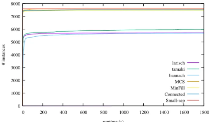
0 1000 2000 3000 4000 5000 6000 7000 8000 0 200 400 600 800 1000 1200 1400 1600 1800 # ins tances runtime (s) larisch tamaki bannach MCS MinFill Connected Small-sep
Fig. 1. The cumulative number of decomposed instances.
exact algorithms confirmed these practical limitations [20]. However, these limitations are questioned by very recent works stimulated by the two first PACE challenges [10] and which improve significantly these approaches. Indeed, between the two iterations of the PACE challenges (i.e. between 2016 and 2017), an improvement of two orders of magnitude for runtime has been observed. So much so that now, the best algorithms can process graphs of several hundreds of vertices in a few dozens of seconds.
These recent advances lead us to reconsider the solving of graphical models by trying to exploit these optimal de-compositions. We must indeed now assess their scalability on real-world instances. This must be done according to two criteria: on the one hand, their ability to decompose real-world instances, and the runtime they need for that, and, on the other hand, the real impact of the use of optimal decompositions on the effective solving of these instances. This second point is also crucial because it has been observed experimentally that the quality of a decomposition method is not only related to the value of the width, but also to other structural criteria of the decomposition, as well as to the nature of the problem to solve [12]. Moreover, decomposition algorithms dedicated to the efficiency of solving graphical models have been recently introduced [9], [21]. The first one called Connected, calcu-lates decompositions guaranteeing that subgraphs induced by clusters are connected (it is called H2 in [9]). The second
one we call Small-sep calculates decompositions minimizing simultaneously w and sep (it is called H5 in [21]). So, we
evaluate now the approach to decompose graphs considering also such algorithms.
B. Ability to Compute Decomposition and Quality
First we describe our experimental protocol. We exploit the three implementations of exact methods for computing optimal tree decompositions, proposed to the PACE 2017 challenge [10]. We call them larisch, tamaki and bannach like in this challenge. Regarding the heuristic methods, we use MCS [8], MinFill [6], [7], Connected [9] and Small-sep [21] that we have implemented.
For the benchmark, we select 7,597 CSP instances en-coded in the XCSP3 format [22] as follow from the XCSP3
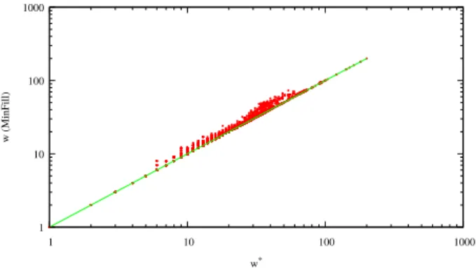
1 10 100 1000 1 10 100 1000 w (MinF ill) w*
Fig. 2. The width obtained with MinFill vs the treewidth.
database1. First, as we aim to compare the decomposition
methods, we limit our study to instances whose primal graph is not a complete graph. Then, the selection is refined accord-ing to solver restrictions. So, only instances with intention, extension, all-different, sum or element constraints are kept. The selected instances have between 6 and 28,161 variables (vertices) and between 5 and 285,685 constraints (edges or hyperedges) whose arity ranges between 2 and 931. It results that the primal graphs have between 5 and 12,547,224 edges. The experiments are performed with Intel Xeon processors 2.4 GHz and we allocated a slot of 30 minutes for decomposing each instance as for the PACE 2017 challenge.
Figure 1 shows the cumulative number of decomposed instances for each decomposition method. Unlike PACE 2017, no exact method is able to decompose all the instances. Then tamaki, which finishes at the second place at PACE 2017, is clearly the best exact method with about 79% of the considered instances which are decomposed against 75% for bannach and larisch. Afterwards, the gap between exact methods and heuristic ones remains important. Indeed, heuristic methods are able to decompose significantly more instances since the percentage of decomposed instances ranges between 98% (MinFill) and 100% (Small-sep).
Regarding the runtime, we can note that all the methods are quite efficient. Indeed, all the methods (including exact ones) require less than 120 s to process most of the decomposed instances. Finally, the main drawback of exact methods is the scalability. If the exact methods treat 92% of the instances having at most 300 vertices, they only decompose 7% of the instances with more than 300 vertices.
We now consider the structural parameters of the produced tree decompositions. If, by construction, the width of a tree decomposition produced by Connected or Small-sep are often far than the treewidth, we can note that the obtained widths for MinFill or MCS are often close. For example, if we consider the 5,996 instances which are optimally decomposed by one of the exact methods, we observe that MinFill computes an optimal decomposition for 3,638 instances. For illustration, we provide in Figure 2 a comparison between the width obtained with MinFill and the treewidth. So, MinFill turns
1See http://xcsp.org/series 0 1000 2000 3000 4000 5000 6000 7000 0 200 400 600 800 1000 1200 1400 1600 1800 #ins tances runtime (s) larisch tamaki bannach MCS MinFill Connected Small-sep VBS
Fig. 3. The cumulative number of solved CSP instances.
to be a good solution for computing a relevant approximation of the treewidth. Concerning the parameter sep of the largest intersection between two clusters, we notice that sep is equal to the width for many decompositions produced by exact methods (more than 60% of the instances), MinFill or MCS (about 30%). For Connected and Small-sep, this phenomenon may occur but is more seldom (e.g. 0.6% for Small-sep).
IV. EVALUATION FROMCSP SOLVINGVIEWPOINT
A. Experimental Protocol
As indicated in the previous section, we used the same instances, that is to say, the benchmark 7,597 instances coming from XCSP3 database. Among these instances, some are real-world instances (e.g. RLFAP or Renault) or have a size similar to one of real-world instances.
We consider two solving algorithms, based on BTD, namely BTD-MAC+RST [23] and BTD-MAC+RST+Merge [21]. The latter is the solving algorithm exploiting tree decomposition which leads to solve the largest number of instances. However, to reach this goal, it may alter the considered decomposition by merging some clusters together. So, it may endanger the op-timality of the initial decomposition (if so) during the solving. That is why we also assess the behavior of BTD-MAC+RST for which the decomposition remains unchanged during the search (except the root cluster which may be modified at each restart). Note that the setting of BTD (variable heuristic, root cluster heuristic, . . . ), except the tree decomposition method, is one described in [24]. We exploit the implementation of BTD-MAC+RST+Merge and Small-sep [24] available from the first XCSP3 Competition2. We add to it the ability to handle the optimal tree decompositions produced by larisch, tamaki and bannachmethods.
As indicated before, the experiments are performed with Intel Xeon processors 2.4 GHz and for each pair decomposi-tion/solving algorithm, we allocated a slot of 30 minutes for decomposing and solving each instance within the limit of 12 GB of memory.
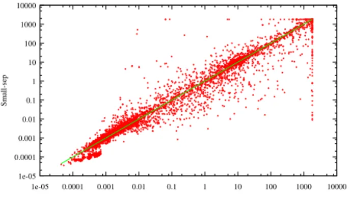
1e-05 0.0001 0.001 0.01 0.1 1 10 100 1000 10000 1e-05 0.0001 0.001 0.01 0.1 1 10 100 1000 10000 Small-sep tamaki
Fig. 4. Tamaki vs Small-sep w.r.t. the solving time (in s) for CSP instances.
0.0001 0.001 0.01 0.1 1 10 100 1000 10000 0.1 1 10 100 1000 10000 Small-sep tamaki
Fig. 5. Tamaki vs Small-sep w.r.t. the global runtime (in s) for CSP instances.
B. Experimental Results
In this part, we assess the relevance of the computed decompositions with respect to the solving efficiency.
If our experiments are achieved with the two algorithms BTD-MAC+RST and BTD-MAC+RST+Merge, we only pro-vide the results observed for BTD-MAC+RST by lack of place. On the one hand, the observed trends are the same for the two solving methods, except that, for each decomposition method, BTD-MAC+RST+Merge solves more instances than BTD-MAC+RST. On the other hand, BTD-MAC+RST has the advantage to preserve the considered decomposition and so its optimality (if so).
We first consider the cumulative number of instances which are solved by BTD-MAC+RST with each decomposition al-gorithm. As depicted in Figure 3, BTD-MAC+RST solves more instances when the decomposition is computed with a heuristic method than with an exact one. Such a result was foreseeable since heuristic methods are able to decompose more instances. For instance, BTD-MAC+RST with tamaki, which is again the best exact method, solves 5,221 instances among the 5,989 instances which are decomposed thanks to tamaki. In the same time, BTD-MAC+RST with a heuristic method solves between 960 and 1,018 additional instances (respectively for MCS and Small-sep), while the virtual best solver (VBS) treats successfully 1,159 additional instances. Note that BTD-MAC+RST with Small-sep and the VBS have clearly a close behavior.
When observing that BTD-MAC+RST with an exact
de-composition method successes very often in solving the in-stance provided that the inin-stance is decomposed, it seems to be natural to study the solving time (i.e. the runtime excluding the decomposition time). So Figure 4 compares the solving time of BTD-MAC+RST with tamaki against its solving time with Small-sep. Of course, by definition, such a figure excludes the instances which are not decomposed by tamaki. We remark that for 41% of the 5,873 considered instances, the solving with tamaki is as efficient as one with Small-sep, whilst, for 33% of the instances, BTD-MAC+RST with Small-sep per-forms better. Finally, the cumulative runtime for the instances solved by BTD-MAC+RST for both decomposition methods is 149,898 s for Small-sep against 172,571 s for tamaki. These results contradict the complexity analysis which claims that the smaller the width is, the more efficient the solving is. Indeed, solving a CSP instance thank to an optimal decomposition is often less efficient than exploiting a heuristic decomposition. This observation is even strengthened if we take into account both the decomposition step and the solving step. Indeed, in this case, exploiting a decomposition heuristic clearly appears to be the best solution. As shown in Figure 5, which compares the global runtime of BTD-MAC+RST with tamaki against its runtime with Small-sep, BTD-MAC+RST with Small-sep is clearly more efficient than with tamaki. As an illustration, 77% of the instances are solved more efficiently with Small-sep while BTD-MAC+RST with tamaki performs better only for 5% of the instances. Moreover, BTD-MAC+RST with tamakirequires 300,366 s to process all the instances solved for both decomposition methods, while it needs only 156,945 s with Small-sep. To conclude, note that the trends observed for WCSP or #CSP solving are similar (not reported here for lack of place), which allows to generalize our observations to a larger class of graphical models.
V. CONCLUSION ANDDISCUSSION
Exploiting an optimal decomposition for solving graphical model instances was unthinkable two years ago. Thanks to the PACE challenge, it seems that it is now possible since, nowadays, algorithms like tamaki can deal with graphs of a few hundred vertices. E.g. tamaki has found optimal decom-positions for 92% of the 6,409 graphs having at most 300 vertices within the 30 minutes timeout. We also observed that an approach like MinFill constitutes a very good heuristic in terms of approximation since it allows to obtain tree decompositions whose width is often close to the optimum as shown in Figure 2. But our experiments also showed that the runtime of the exact algorithms is a major drawback as soon as the graphs consist of several hundreds of vertices. In particular, it has been observed that only 7% of the graphs with more than 300 vertices can be optimally decomposed within 30 minutes. It ensues that, for the moment, exact methods cannot be exploited yet as a general tool for decomposing graphical models and so that the use of heuristic approaches remains necessary for the general case.
This observation is further strengthened when we consider the effective solving of graphical models (in the sense of the
CSP in our experiments). Indeed, as soon as the instances of graphical models have a few hundred variables, the cu-mulated time for decomposing and solving is too important and constitutes a real obstacle to their use comparing to heuristic decompositions (as shown in Figure 3). Moreover, surprisingly, when optimal decompositions are computable by exact methods, they do not guarantee a more efficient solving. Indeed, the solving with such optimal decompositions is often outperformed by the solving with heuristic decomposition (see Figure 4). It had already been observed empirically that the width of a decomposition does not necessarily constitutes the crucial parameter for such solving methods [23]. However this could never be verified before on optimal decompositions.
These results were obtained on the basis of a solving method (BTD) which exploits the tree decomposition and can be considered as an intermediate approach between search (backtracking or branch and bound) and the DP approach. This leads us to question the use of DP methods based on optimal decompositions. Indeed, very often, such solving approaches need memory space close to exp(w∗) because we observed that w∗ = sep for more than 60% of the instances of our benchmark. Moreover, [12] point out that the treatment of instances of small size (a real-world benchmark called ”Vienna” with n = 138) with a limited treewidth (w∗ = 5 for these instances) can requires several hours of calculation to be solved when using a DP approach.
All these observations lead us to suggest different tracks for future investigations. Sure, the first one would be to improve the efficiency of exact methods, but it will most likely lead to decompositions for which sep will be very close to w∗. Secondly, by observing that heuristics (like Small-sep) produce decompositions which are very relevant for the solving step while obtaining widths often far from w∗, one can consider that such heuristics are a crucial object of study for the solving of real-world instances of graphical models. In addition, it seems relevant to study mixed approaches. Indeed, since from now on, it is possible to decompose optimally graphs a few hundred vertices, it could be useful to exploit the exact algorithms locally as routines in order to decompose the largest clusters so as to overcome the defects of the heuristics. This could lead to methods that are both time-efficient and more effective for solving.
Among the other tracks, one must mention an original work that uses machine learning techniques to identify the best decompositions to be used for the practical solving [12]. However, in conclusion, the authors highlight the current limitations of this kind of approach due to the preliminary training step necessary for its use.
Finally, we have now to better identify the properties that a decomposition must satisfy to ensure an efficient solving of a graphical model instance. Indeed, a heuristic like Small-sepappears to be efficient for both decomposing large graphs (all the considered instances have been processed), and, above all, solving associated instances. So, for future works, we have to highlight the parameters which allow us to produce the best decompositions in view of the solving. If some of
them are probably related to the structure (like w and s, or local properties like for the heuristic Connected), taking into account the semantic of the instances now seems the most promising research track.
ACKNOWLEDGMENT
This work has been funded by the french Agence Nationale de la Recherche, reference ANR-16-C40-0028.
REFERENCES
[1] V. Bertele and F. Brioschi, Nonserial Dynamic Programming. Elsevier, 1972.
[2] N. Robertson and P. Seymour, “Graph minors II: Algorithmic aspects of treewidth,” Algorithms, vol. 7, pp. 309–322, 1986.
[3] R. Dechter, Reasoning with Probabilistic and Deterministic Graphical Models: Exact Algorithms. Morgan and Claypool Publishers, 2013. [4] ——, Constraint processing. Morgan Kaufmann Publishers, 2003. [5] S. Arnborg, D. Corneil, and A. Proskuroswki, “Complexity of finding
embeddings in a k-tree,” SIAM Journal of Disc. Math., vol. 8, pp. 277– 284, 1987.
[6] D. J. Rose, “A graph theoretic study of the numerical solution of sparse positive definite systems of linear equations,” in Graph Theory and Computing. Academic Press, 1972, pp. 183–217.
[7] U. Kjaerulff, “Triangulation of Graphs - Algorithms Giving Small Total State Space,” Judex R.R. Aalborg., Denmark, Tech. Rep., 1990. [8] R. Tarjan and M. Yannakakis, “Simple linear-time algorithms to test
chordality of graphs, test acyclicity of hypergraphs, and selectively reduce acyclic hypergraphs,” SIAM Journal on Computing, vol. 13 (3), pp. 566–579, 1984.
[9] P. J´egou, H. Kanso, and C. Terrioux, “An Algorithmic Framework for Decomposing Constraint Networks,” in ICTAI, 2015, pp. 1–8. [10] H. Dell, C. Komusiewicz, N. Talmon, and M. Weller, “The PACE 2017
Parameterized Algorithms and Computational Experiments Challenge: The Second Iteration,” in IPEC, 2018, pp. 30:1–30:12.
[11] G. Gottlob, N. Leone, and F. Scarcello, “A Comparison of Structural CSP Decomposition Methods,” AIJ, vol. 124, pp. 243–282, 2000. [12] M. Abseher, N. Musliu, and S. Woltran, “Improving the Efficiency of
Dynamic Programming on Tree Decompositions via Machine Learning,” JAIR, vol. 58, pp. 829–858, 2017.
[13] P. J´egou and C. Terrioux, “Hybrid backtracking bounded by tree-decomposition of constraint networks,” AIJ, vol. 146, pp. 43–75, 2003. [14] R. Dechter and R. Mateescu, “The Impact of AND/OR Search Spaces on Constraint Satisfaction and Counting,” in CP, 2004, pp. 731–736. [15] S. de Givry, T. Schiex, and G. Verfaillie, “Exploiting Tree
Decomposi-tion and Soft Local Consistency in Weighted CSP,” in AAAI, 2006, pp. 22–27.
[16] B. Hurley, B. O’Sullivan, D. Allouche, G. Katsirelos, T. Schiex, M. Zyt-nicki, and S. de Givry, “Multi-language evaluation of exact solvers in graphical model discrete optimization,” Constraints, vol. 21, no. 3, pp. 413–434, 2016.
[17] A. Koster, “Frequency Assignment - Models and Algorithms,” Ph.D. dissertation, Univ. of Maastricht, 1999.
[18] K. Shoikhet and D. Geiger, “A practical algorithm for finding optimal triangulation,” in AAAI, 1997, pp. 185–190.
[19] V. Gogate and R. Dechter, “A complete anytime algorithm for treewidth,” in UAI, 2004, pp. 201–208.
[20] H. L. Bodlaender, F. V. Fomin, A. M. C. A. Koster, D. Kratsch, and D. M. Thilikos, “On exact algorithms for treewidth,” ACM Trans. Algorithms, vol. 9, no. 1, pp. 12:1–12:23, 2012.
[21] P. J´egou, H. Kanso, and C. Terrioux, “Towards a Dynamic Decompo-sition of CSPs with Separators of Bounded Size.” in CP, 2016, pp. 298–315.
[22] F. Boussemart, C. Lecoutre, and C. Piette, “XCSP3: an integrated format for benchmarking combinatorial constrained problems,” CoRR, vol. abs/1611.03398, 2016.
[23] P. J´egou and C. Terrioux, “Combining restarts, nogoods and bag-connected decompositions for solving CSPs,” Constraints, vol. 22, no. 2, pp. 191–229, 2017.
[24] P. J´egou, H. Kanso, and C. Terrioux, “BTD and miniBTD,” in XCSP3 Competition, 2017.