HAL Id: hal-01294943
https://hal.archives-ouvertes.fr/hal-01294943
Submitted on 30 Mar 2016
HAL is a multi-disciplinary open access
archive for the deposit and dissemination of
sci-entific research documents, whether they are
pub-lished or not. The documents may come from
teaching and research institutions in France or
abroad, or from public or private research centers.
L’archive ouverte pluridisciplinaire HAL, est
destinée au dépôt et à la diffusion de documents
scientifiques de niveau recherche, publiés ou non,
émanant des établissements d’enseignement et de
recherche français ou étrangers, des laboratoires
publics ou privés.
Florian Mercier, Stéphane Bonelli, Frederic Golay, F. Anselmet, P. Philippe,
R. Borghi
To cite this version:
Florian Mercier, Stéphane Bonelli, Frederic Golay, F. Anselmet, P. Philippe, et al.. Numerical
mod-elling of concentrated leak erosion during Hole Erosion Tests. Acta Geotechnica, Springer Verlag,
2015, 10 (3), pp.319-332. �10.1007/s11440-014-0349-5�. �hal-01294943�
Postprint accepted - Acta Geotechnica
Numerical modelling of concentrated leak
erosion during Hole Erosion Tests
Mercier F.
(1),(2), Bonelli S.
(1), Golay F.
(3), Anselmet F.
(4),(5), Philippe P.
(1), Borghi R.
(5)(1)Irstea, 3275 Rte Cézanne, CS 40061, 13182 Aix-en-Provence Cedex 5, France (2)
GeophyConsult, Savoie Technolac, 12 allée du lac de Garde, BP 231, 73374 Le Bourget du Lac Cedex, France
(3)Imath, Avenue de l’Université, BP 20132, 83957 La Garde, France (4)
IRPHE, Technopôle de Château-Gombert, 49 rue Joliot Curie, BP 146, 13384 Marseille Cedex 13, France
(5)
ECM, Technopôle de Château-Gombert, 38 rue Frédéric Joliot-Curie, 13451 MARSEILLE Cedex 20
Corresponding Author:
Fabienne Mercier, Ph. D. – [email protected]
IRSTEA, 3275 Rte Cézanne, CS 40061 13182 AIX EN PROVENCE Cedex 5 FRANCE
Tel: +33 442 669 948 Fax: +33 442 668 865
Abstract: This study focuses on the numerical modelling of concentrated leak erosion of a cohesive soil by a
turbulent flow in axisymmetrical geometry, with application to the Hole Erosion Test (HET). The numerical model is based on adaptive remeshing of the water/soil interface to ensure accurate description of the mechanical phenomena occurring near the soil/water interface. The erosion law governing the interface motion is based on two erosion parameters: the critical shear stress and the erosion coefficient. The model is first validated in the case of 2D piping erosion induced by a laminar flow. Then, the numerical results are compared with the interpretation model of the Hole Erosion Test. Three HETs performed on different soils are modelled with a rather good accuracy. Lastly, a parametric analysis of the influence of the erosion parameters on erosion kinetics and evolution of channel diameter is conducted. Finally, after this validation by comparison with both the experimental results and the interpretation of Bonelli et al. [2], our model is now able to reproduce accurately the erosion of a cohesive soil by a concentrated leak. It also gives access to a detailed description of all the averaged hydrodynamic flow quantities. This detailed description is essential in order to achieve a better understanding of the erosion processes.
Key-words: Concentrated leak erosion; critical shear stress; erosion coefficient; turbulent flow modelling;
1.
Introduction
Numerical modelling of erosion phenomena has been studied intensively over the last 20 years. Mainly, two approaches to erosion modelling have been developed, both of which are well-adapted to a flow of water on a granular soil. At the scale of a continuous medium, Vardoulakis et al. [16] proposed a mechanically-based numerical simulation approach where a fluidised solid phase is introduced in a model providing smooth transition between solid and liquid phases. The erosion of the solid phase is represented by a source term that describes the exchanges of mass between the three phases. The second approach was proposed by Ouriemi et al. [12]. They proposed a diphasic model in which solid and liquid phases are in direct interaction. A source term in the momentum conservation equation described the momentum fluxes between the two phases. In both approaches, the permeability of the granular soil must be sufficiently high to allow the development of such a fluidised solid phase. The fluid, the intermediate zone and the granular medium are described by Navier-Stokes, Brinkman and Darcy models, respectively. However, by contrast to granular soils, most cohesive soils have extremely low permeability, making the influence of the water flow in the soil completely negligible. Therefore, the solid/flow interface can be considered as a singular interface with a negligible thickness. In this case, the erosion phenomenon is simply described by the flux of eroded mass crossing this interface [5, 9].
With a slow erosion kinetics in comparison to the typical flow velocity, the presence of eroded particles in the flow phase can be neglected. The diphasic model can be simplified to a monophasic model. Golay et al. [8] developed such a monophasic erosion model adapted to an incompressible Stokes flow and where the fictitious domains approach was employed with the Level-Set method [11]. None of this numerical model permits to model the erosion of a cohesive soil by a turbulent flow.
Bonelli et al. [2] developed an analytical model to describe piping erosion by a turbulent flow in the specific configuration of the Hole Erosion Test (HET). The HET is a test apparatus that provides the erosion parameters of a soil sample [17]. Bonelli et al. [3] then proposed an improved interpretation model of the HET based on this analytical piping erosion model. In the present study, a numerical model of piping erosion is performed for a channel in cohesive soil subjected to a turbulent flow. A comparison is made between the results of our numerical model and the semi-empirical approach of the Hole Erosion Test by Bonelli et al. [3]. In the first part of this paper, emphasis will be given to the development and validation of the numerical model. Then, the numerical results obtained for the modelling of three HETs performed on different soils will be compared to the experimental results. Pressure field, velocity magnitude and shear stress distribution will be discussed. Developing such a numerical model permits to access the flow mechanical quantities, that cannot be estimated by analytical models. This could lead to a better understanding of the erosion processes.
The paper is organised as follows: we first describe the physical model in section 2 and then the numerical model in section 3. This numerical model of piping erosion is validated for laminar flow conditions in section 4. In section 5, we present the results of the numerical model with a turbulent flow in the HET configuration. Three HETs performed on different soils are modelled, and the numerical results are compared to the experimental ones. Also a parametric analysis allows the validation of the numerical model. Finally, a discussion of the results will be presented in section 6.
2.
Physical model
2.1
Decoupled resolution
The orders of magnitude deduced by Bonelli et al. [4], as part of their study of diphasic flows with erosion and transport, allow several simplifications. First, as the erosion kinetics is slow in comparison to the typical fluid velocity, the flow can be considered as steady with respect to the erosion time scale. The resolution of the flow equations can therefore be decoupled from the resolution of the interface equations. Then, considering the orders of magnitude of the flow parameters used in the analytical model of Bonelli et al. [4], the assumption of a diluted flow allows ignoring the presence of eroded particles within the flow. Finally, the influence of the flow within the solid phase is neglected as a result of the assumption of saturated soil.
Therefore, the physical model describing the flow is considered as monophasic and the boundary of the fluid domain is considered as stationary during the computation of the fluid phase. The solid phase is only considered through its interface with the fluid calculation domain. The physical model of the solid phase does not consider any evolution of the flow during its calculation.
2.2
Equations at the interface
The most commonly used erosion law for a cohesive soil is a linear threshold law that takes the following form:
( ) if 0 else d c c k c! =#$ ! !" ! !> % on ! (1)
where ! =! !! , !=T n! " ! !(n T n n) is the shear stress on !, n is the unit vector normal to ! and oriented towards the soil, T is the Cauchy stress tensor, and c! is the velocity of the mobile interface. The erosion parameters of the soil are the critical shear stress !c (Pa) and the erosion coefficient kd (m².s/kg).
2.3
Field equations
The fluid domain is denoted !w,
u
is the mean velocity of the flow and !w is the fluid density. The Navier-Stokes turbulent fluid flow equations read:0 ( ) w t ! ! " = # $ % & ' + ! " (=! " $ )+% *, -u u u u T in !w (2) with T=!pI+2µwD R+ in !w (3) 1 ( ) 2 T ! " = $# + # % D u u , R="!wu!#u ! (4)
where p is the mean static pressure, µw the fluid molecular viscosity, D the symmetrical part of the mean velocity gradient, I the identity tensor and R the turbulent stress tensor which accounts for momentum transfer by velocity fluctuations.
The Navier-Stokes equations are solved by the Reynolds Averaged Navier-Stokes method, which induces the turbulence closure problem. In the case of channel geometry, the turbulent flow regime is accurately described by a k!! turbulence model [13]. The k!! turbulence model of Shih et al. [15] is based on the Boussinesq hypothesis, which introduces a turbulent viscosity µt through the following relation:
2 2 ( ) 3 w t wk ! ! ! µ ! " u #u = D u " I (5)
where k=u u! !" / 2 is the kinetic energy of velocity fluctuations proportional to the trace of the Reynolds stress tensor. Finally, the turbulent viscosity can be written as:
2 t w k Cµ µ ! " = (6)
where !w =µ "w/ w is the kinematic viscosity of the fluid, !=" # $#"w u! u is the rate of the viscous dissipation !
of turbulent kinetic energy and Cµ is a constant which may sometimes be a function of the mean deformation of
k and ! .
The transport equations for k and ! are the following:
( ) t w w k k k k k k P Y t µ ! µ " !# $ " %
! + & ' "=& ' + & + (
)+ , * )% * - u. )-/ 0 *. (7) ( ) t w w P Y t ! ! ! µ ! " ! µ ! # !# $ " %
! + & ' "=& ') + & *+ (
+ ,
)% *
- u. )-/ 0 *. (8)
where Pk (resp. P!) is the source term for the production of k (resp. ! ) due to the mean velocity gradient and where Yk (resp. Y!) is the dissipation of k (resp. ! ) due to turbulence.
3.
Numerical modelling
3.1
Fluid/soil interaction modelling
The fluid phase is usually described by an Eulerian approach and the solid phase by a Lagrangian one. Two types of resolution methods can be used. The first is a fully Eulerian approach where the solid phase equations are written as the fluid phase ones. The mobile interface is captured with a fixed mesh. An interface function, such as a Level-Set function [11], is introduced to separate the fluid and solid domains independently of the mesh. A precise description of the flow variables at the interface cannot be given by the Eulerian approach since the wall functions are poorly described and overall remeshing is needed to improve the accuracy of the model close to the interface. The second type of resolution method is a mixed Eulerian-Lagrangian approach [7]. Both phases are described in a mobile mesh and the mobile interface is tracked. The fluid phase equations are first computed by an Eulerian approach independently of the solid resolution model. Then the equations governing the solid phase are solved on the basis of the results found for the fluid phase with a Lagrangian approach. The mesh of the fluid domain is distorted as a function of the solid phase results. This method is then limited by mesh distortion, leading to the need for remeshing which can be very costly in terms of computation time. However, the main advantage of the mixed Eulerian-Lagrangian approach is that mechanical quantities, such as shear stress, are computed with great accuracy, even close to the solid interface. This is the reason why this mixed approach was chosen here.
3.2
Erosion law
After the resolution of the Navier-Stokes equations in the fluid domain using the finite volume method, the positions of the nodes of the interface are updated by an explicit Euler scheme:
( ) if ( ) ( ) 0 else d c c t k t+!t = t +#$! ! !" ! !> % n x x (9)
where x( )t is the position vector at time t of a node of the interface. Once the position of the fluid/soil interface has been updated, the fluid calculation domain is remeshed and interpolations are performed from the old cells to the new ones to obtain a mesh adapted to the new configuration. A large number of remeshing procedures is needed to model the entire erosion process. After several dozen local deformations and refinements, the meshing is so unstructured that it is necessary to perform a global remeshing associated with an interpolation of the flow fields. The complete modelling of erosion induced during an HET requires about one month’s calculation time on a cluster of 8 CPUs with Intel Xeon EMT64 3.2 GHz dual processors.
3.3
Turbulent wall laws
The fluid domain near the soil/water interface can be divided into three regions. Closest to the interface is located a viscous sub-layer where viscous effects are dominant. Far from the wall is a log-law region or inertial fully turbulent sub-layer, where turbulent effects dominate. In between, a buffer sublayer or mixing zone is governed by both viscosity and turbulence.
The dimensionless distance from the centre of the first cell at the wall ( y+) and the friction velocity at the wall (U!) are given respectively by:
w w U y y " ! µ + = , w w U! ! " = (10)
where y is the distance from the centre of the first cell in contact with the wall.
The k-! turbulence model is known to be accurate far from the walls but additional equations have to be introduced to solve the fluid phase near a wall. The enhanced wall treatment approach is used. If y+>300 the
turbulence model is applied directly. The mean velocity components are deduced from a log-law if 30<y+<300,
whereas if y+<30, a linear stress/deformation relation corresponding to the viscous regime is applied [10].
Concerning the enhanced wall treatment approach, a two-layer model is applied where the computation domain is divided into two zones, one fully turbulent and the other sensitive to viscous effects. The frontier between these two zones is defined by:
Rey w 200 w y k ! µ = ! (11)
If Rey>200, the flow is assumed to be fully turbulent and the k-! turbulence model can be used. Otherwise, the
one-equation model of Wolfshtein [18] is used. The turbulent kinetic energy is then calculated with transport equations and the turbulent viscosity is determined using the characteristic length scale lµ introduced by Chen et
al. [6].
The numerical model developed will be first validated on a laminar flow case. We consider a channel eroded by a flow with a constant pressure drop. No equilibrium state can be reached, as the erosion phenomenon diverges. Then, the model will be applied to several Hole Erosion Tests. A pipe will then be eroded by a flow with a constant flow rate, so that the erosion process will end on an equilibrium state.
4.
Validation of the erosion model with a laminar flow
4.1
Theoretical solution
The erosion of a cohesive soil by a laminar flow in a 2-dimensional configuration can be used as a benchmark to test our numerical modelling. Indeed, this simple case corresponds to the well-known plane Poiseuille flow whose theoretical solution for the horizontal velocity of the flow u reads:
( )
( )
( )
2 2 2 3 1 1 2 av 2 w R t r p r u u R t x R t ! # $ " % ! # $ " & ' & ' = & ()) ** '= % & ()) ** ' + , + , - . µ - . (12) where R(t) is the channel diameter at time t, µw is the fluid viscosity, uav is the average horizontal velocity andp is the pressure field. The wall shear stress ! , deduced from the horizontal velocity is:
( )
3 w avu R t = µ
! (13)
For a constant pressure drop, the resolution of the erosion law in Eq. (1) gives [4]:
( )
0 0 0 1 er t t c c R t L L e R R p R p ! ! ! " = +$ # % & ' & ( (14) er d L t k p = ! (15)with R0 being the initial diameter of the erodible channel, ter a characteristic erosion time scale and L the length of the channel.
4.2
Numerical results
The data used as boundary conditions of the numerical model are the following: the radius of the channel is
R0=0.5 mm and a pressure differential equal to 10!2 Pa is applied. The characteristics of the soil are:
6 2 10 m .s/kg d
k = ! , !c=0 Pa. The numerical model is formulated for two channel lengths: L1=1 cm and 2 1 m
L = . The meshing used is a uniform grid whose dimensions are 50x500 for the 1 cm long channel and 20x20,000 for the 1 m long channel, ensuring the independence of the results from the mesh density. To get rid of the flow establishment length, it is preferable to impose velocity profiles at the inlet. These profiles have to correspond to the pressure chosen, which will then depend on height of the channel as a function of time, cf. Eq. (12). The extraction of the diameter after each mesh deformation and its implementation in the input parameters is therefore necessary at each erosion time step.
The numerical results obtained for the channels of 1 cm and 1 m lengths are compared with the theoretical solution of equation (14). The erosion process never stops as the pressure condition is imposed at the inlet. On the contrary, the erosion accelerates exponentially through time, as described by equation (14). For the two modelled channel lengths, the correspondence between the numerical and theoretical results is very good. The relative error between the numerical results obtained and the theoretical solution is always lower than 2%. The
pertinence of the results obtained in the framework of the 2D laminar piping erosion model is an important element used to validate the modelling method developed in section 2.
5.
Modelling Hole Erosion Tests
5.1.
Characterisation of the soils tested
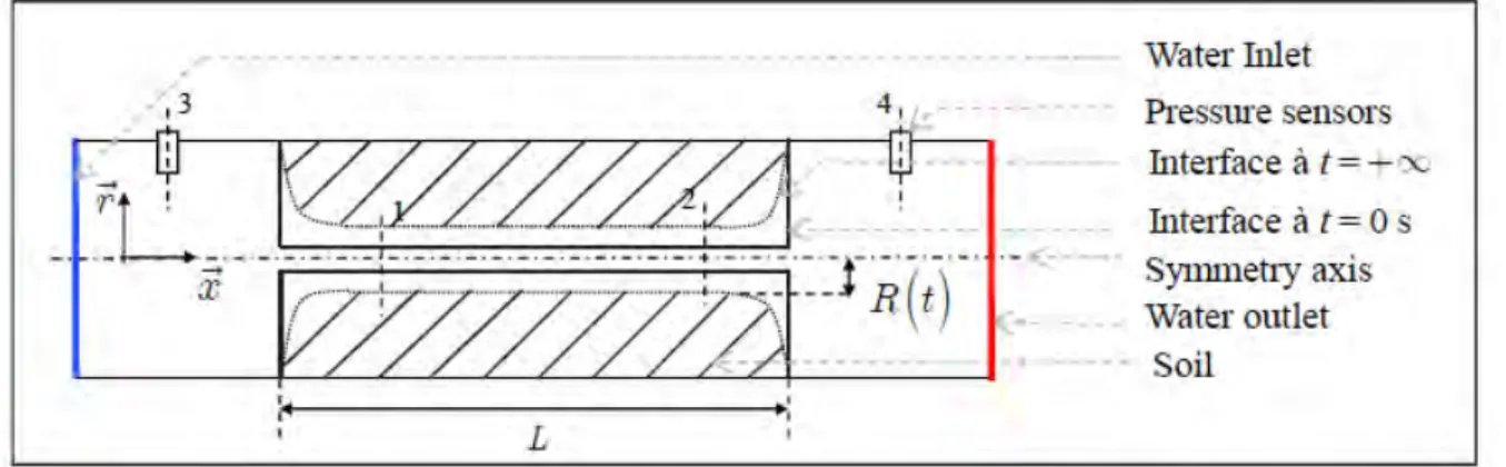
Three models of Hole Erosion Tests were run to obtain validations of the modelling method developed in section 2. A scheme of the experimental device is shown in Figure 1, in which the notations used are also explained. A fixed flow rate of water penetrates the inlet cylinder, and then transits through the soil sample via the initial default previously drilled along the sample. The flow passes through an abrupt narrow section to enter the channel through the soil sample. This channel presents uniform diameter at zero erosion time. Then the flow at the outlet of the soil sample passes through a sudden widening and leaves via a cylinder of diameter equal to the one of the inlet cylinder. These tests were performed on three distinct soils named A, D and E. The boundary conditions are: the outlet pressure, which equals the atmospheric one, the initial channel radius of
3 0 3.10 m
R = ! , the inlet flow rate and the sample length, presented in Table 1.
Soil A was sampled from an existing dike and disturbed. Soils D and E are calibrated test soils, and the experimental data were obtained from the study performed by Benahmed and Bonelli [1]. Soil A is composed by silts with broken stones, soil D is constituted wholly of white kaolinite and soil E is a mixture of proclay (30%) and Hostun sand (70%). The results of the identification tests of these soils are presented in Table 2 (photographs of the soils are shown in Figure 3). The erosion parameters of soils A, D and E are the critical shear stress and the erosion coefficient presented in Table 1. The erosion coefficient can also be presented through Fell’s erosion index defined as follows: IHET =!log(C Ce 0) with Cebeing Fell’s erosion coefficient such that
e d s
C =k ! and C0 =1 s/m [17]. According to Fell’s classification of erodibility, the erosion velocity of soils A and E is very rapid (2<IHET <3), and moderately rapid for the soil D (3<IHET <4). The choice of modelling the Hole Erosion Tests carried out on these three soils was made as a function of their very different natures, and regarding the different flow parameters fixed for these tests. The characteristic erosion parameters, critical shear stress and erosion coefficient of the soils are, however, quite similar. Figure 2 shows the differences observed experimentally on the evolution of the pressure differential between the cross-sections named location#3 and location#4 as a function of time. Figure 1 shows the positions of these cross-sections, corresponding to the pressure sensors locations. The erosion kinetics in the case of soil E is faster than that of soil A, which is itself faster than that obtained for soil D. This is consistent with the relative positions of the soils in Fell’s classification. In the case of soil E, the erosion process stops about four times earlier than for soil D. The volumes of the eroded soils were measured at the end of the tests. For the HET performed on soil A, the volume of the eroded soil measured was about 21 cm3, for a sample length of 12 cm. For soils D and E, the volumes of the eroded soil were close to 45 cm3 and 15.5 cm3 respectively, for a sample length of 15 cm. Photographs of the soil samples before and after the Hole Erosion Tests are presented in Figure 3. The diameter of the sample was 8 cm with the initial hole (6 mm). The diameters upstream of the erodible channel at the end of the erosion process were 2, 2.5 and 1.8 cm, to within 1 mm, for soils A, D and E, respectively. This means that the maximum diameters reached at the end of the erosion process were between 6 and more than 8 times the diameter of the initial default.
5.2.
Independence of results with mesh density
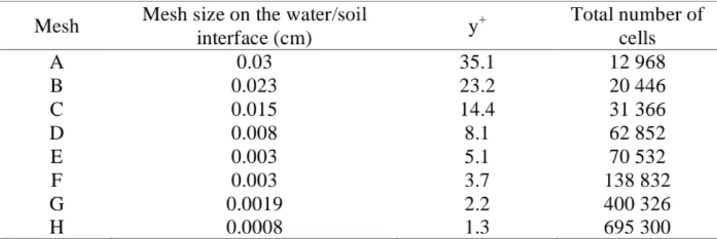
A 2D axisymmetric numerical model is formulated. The results presented below correspond to the HET performed on soil A. In fact, the independence of the results from mesh density for the tests performed on soils D and E was validated in the same way as for the case of soil A. The different models relating to the HET tests were formulated with the k-ε realizable turbulence model. The study of the independence of the results in relation to mesh density is performed for eight meshes whose total number of cells varies from 10 000 to about 700 000. At the water/soil interface, the size of a face separating two nodes varies inversely proportional to the number of cells: from 8.10-6 m to 3.10-4 m, as shown in Table 3. The mesh is then expended to the rest of the domain by expansion factors of 1.1 or 1.2 as depending on the mesh considered. The meshes tested are entirely composed of triangular cells, to ensure the continuity of the mesh along the whole axis of symmetry. The entire calculation domain will be affected for the case with erosion causing mesh deformations.
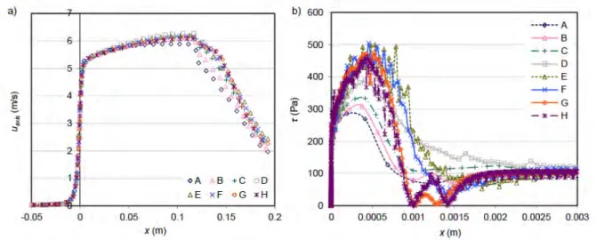
Figure 4 illustrates the study on the independence of the results regarding mesh density. Figure 4a presents the results for the norm of the velocity taken along the axis of symmetry, for the different meshes tested. Figure 4b
shows a close-up of the curves presenting the shear stress at the first geometric singularity of the water/soil interface, namely the sudden narrowing of the pipe. Once the mesh density equal to or greater than mesh C is reached, the values computed for the different variables along the axis of symmetry are independent of the mesh density to within 10%. This independence is also obtained at the water/soil interface, excluding the two geometric singularities: sudden narrowing and widening. At the singularities, and especially for the sudden narrowing, the results fluctuate considerably (Figure 4b) for a given meshing density if the latter is higher than mesh E. The right angle arising from the sudden narrowing effectively forms a zone that greatly destabilizes the flow. A mesh such as mesh D presents a relative error on the maximum shear stress at the narrowing of about 16%, in comparison to the results given by mesh H. It permits a substantial smoothing of the fluctuations observed for the denser meshes. However, the zone affected by this higher relative error only represents a thirtieth of the horizontal part of the water/soil interface.
Thus it can be estimated that starting from a mesh density equivalent to that of mesh D, the results obtained are independent of the mesh density to within 5% except for about a thirtieth of the horizontal part of the water/soil interface, at the geometric singularities, where the independence of the results regarding the meshing density is slightly lower. Therefore, the numerical model of the piping erosion in this test configuration was performed with mesh D.
5.3.
Results with erosion
The erosion parameters implemented are those obtained experimentally after the HETs performed on soils A, D and E, which are presented in Table 1. The interpretation model of Bonelli et al. [2] has been used to deduce the critical shear stress and the erosion coefficient within more and less 10%. We compare the numerical results obtained with the experimental data and with the analytical results given by Bonelli et al. [2]. This analytical model gives the evolution of different variables in a channel subjected to erosion. The basic equations of the model are as follows for erosion along a pipe submitted to a constant flow:
1/ 4 1/ 4 5/ 4 ( c ) ( c ) c
f !! R! = f !! +!! t! with ( ) 1
(
arctan arctanh)
2 f x = x+ x ! x (16) er t t t = ! , 0 c c ! ! ! = ! ,( )
( )
0 R t R t R = ! (17) 0 2 er d L t k P = ! , 2 12 R P L ! = ! (18)where !0 and !!c are the initial and dimensionless threshold shear stresses, ÄP12 and ÄP0 are the pressure differential in the pipe at t and t=0 s, R t ,
( )
R0 and R t!( )
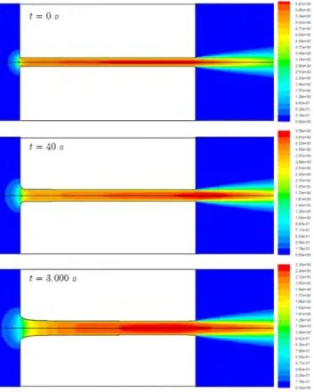
are respectively the radius of the erodible channel of length L at time t, initially, and the dimensionless radius; t, ter and t! are the time, the characteristic erosion time and the dimensionless time. The results obtained with the analytical model depend on the pressure differential between locations 1 and 2 (!P12) at t=0. There are several possible choices in this comparison between the analytical model and the numerical results. This first part of section 5 does not deal with the experimental results. Nonetheless, for the interpretation of this test intended to obtain the erosion parameters, the value of !P12 found experimentally is used in the model of Bonelli et al. [2]. We can also consider the theoretical pressure differential found with Blasius’ formula, the results obtained from complex CFD modelling or our numerical results.Figure 5 illustrates the evolution of the water/soil interface obtained numerically as a function of time in case of soil A. The evolution of the velocity field at the beginning, in the middle (in terms of displacement) and at the end of the erosion process is shown. Despite the relatively low critical shear stress imposed, the erosion of the soil remains very limited for soils D and E, see Figure 6. In the case of the test performed on soil A, the radius obtained in the middle of the erodible pipe was about 4.8 mm. A final radius of 4.3 mm was obtained for soil D and of 4.1 mm for soil E. These values remain very close for the three tests and only range from 1.3 to 1.6 times the initial channel radius. The erosion of the soil is more extended upstream of the channel. With time, the geometric singularity upstream is progressively smoothed and the diameter of the upstream channel becomes larger than the diameter of the downstream channel. The erosion process is progressively stopped in the downstream-upstream direction of the pipe, since the shear stress is higher upstream. The nodes of the interface whose radii are such that the shear stress has become lower than the critical shear stress are no longer displaced. The upstream radius of the channel obtained numerically is about 7.5 mm for soil A, 6 mm for soil D and 6.5 mm for soil E. The results obtained for the geometrical singularity upstream are correct. Given that the meshing is not sufficiently dense to ensure the independence of the results in relation to the meshing (cf. section 5.2), this singularity is very difficult to model properly. Figure 5 shows the acceleration of the fluid along the axis of
symmetry between locations#1 and locations#2 (see Figure 1 for locations positions). At t=0 s, because of the establishment phase of the flow in the pipe, the velocity is larger at location#1 than at location#2. Since the section at location#2 becomes larger than the section at location#1 (t>0 s), the average velocity is no longer constant in between the two sections. The more the erosion process progresses, the more the fluid accelerates downstream but also the more the diameter of the channel increases and, consequently, the more the velocity in the channel decreases. The maximum velocity magnitudes obtained at the end of the erosion process reach 2.4 m/s, 3.1 m/s and 1.5 m/s for the tests on soils A, D and E respectively.
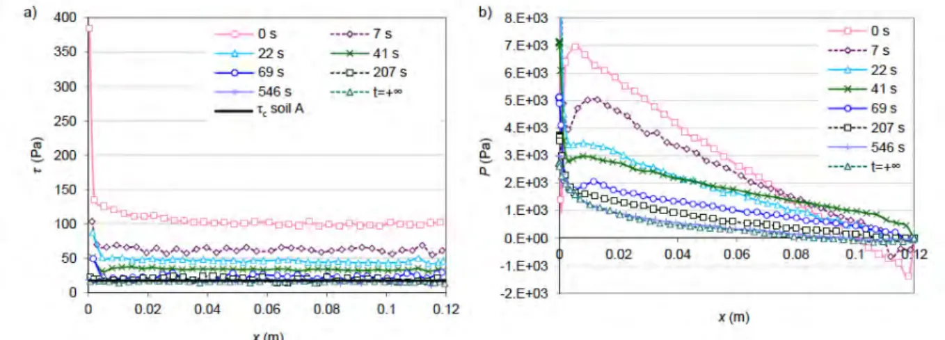
According to the flow rate conservation law, the average velocity of the fluid in the channel evolves in inverse proportion to the square of the diameter. The flow velocity in the channel therefore decreases very quickly as its diameter increases. This explains that the shear stress exerted by the fluid on the soil also decreases very rapidly with the increase of the channel diameter. The shear stress quickly decreases below the threshold shear stress and the erosion process stops at an early stage. An important peak of shear stress is observed at the point where the channel suddenly narrows, as illustrated in Figure 7a in case of soil A. This explains why the erosion is more efficient at this geometric singularity than in the rest of the pipe. Once the geometrical singularity upstream has been passed the shear stresses remain almost constant on the water/soil interface. The shear stress peak is smoothed as the erosion process progresses. Except for the geometrical singularities at the entry and exit of the pipe, the shear stress at the water/soil interface is almost constant. At the end of the erosion process, the shear stress equals the critical shear stress at every point of the soil/water interface. The initial shear stresses of the tests performed on soils A and D are of the same order of magnitude, with !x=6cm !100 Pa. In the case of soil E, the shear stress reaches nearly a quarter of the values found in the two other cases, with !x=6cm!26 Pa. This corresponds to the differences between the flow rates imposed at the inlet, see Table 1, with a much lower inlet flow rate for soil E than that imposed for the two other soils. Having a higher kinetic coefficient and a lower critical shear stress nonetheless permits obtaining a final radius close to that obtained for the two other tests. Figure 8a illustrates the comparison between the numerical results and the model by Bonelli et al. [2] on the evolution of the shear stress for the three tests as a function of the radius of the erodible channel. Although the results obtained in the case of model D are very close to the results of the analytical model, we observed a larger discrepancy for the two other tests. These gaps are due to errors on the initial value of the pressure differential. Figure 8b shows, on the example of soil A, that if a pressure differential corresponding to that obtained numerically is used in the analytical model, the results obtained agree nicely with the numerical results. The numerical results therefore agreed well with the analytical formula defining the stress, Eq. (1.9). Whatever the test considered we observe that the errors between the numerical and analytical results lessen through time, see Figure 8a.
Concerning pressure fields, in spite of the non-uniform evolution of the diameter of the pipe along its length, the pressure decreases almost linearly between location#1 and location#2, as illustrated in Figure 7b for case of soil A. The pressure differential between location#1 and location#2 decreases with time, in accordance to the analytical predictions of Bonelli et al. [2]. As the flow rate entering the channel is constant, the more the channel diameter widens with time, the more the pressure differential decreases. When the shear stress becomes lower than the critical shear stress at the soil/water interface, the erosion process stops and the pressure differential reaches its asymptotic value. The erosion kinetics obtained numerically and analytically also agree well. The evolution of the shear stress also corresponds to those found analytically for the three values of !P0. The evolution of the pressure differential between location#1 and location#2 is compared to the results obtained with the analytical model. Good agreement is observed between the numerical and analytical results, whatever the pressure differential chosen, whether numerical, experimental or theoretical. The relative errors between the numerical results and those of the model of Bonelli et al. [2] are about 5%, 15% and 10% respectively. Same results were obtained for the comparison of the evolution of the channel radius, taken in the middle of the useful length of the channel, showing the good correspondence of the erosion kinetics.
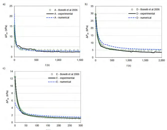
The evolution of the pressure differential between location#3 and location#4 obtained numerically has been compared with the results of the analytical model and the experimental data. The model of Bonelli et al. [2] gives
34 0.27 12
P P
! = ! . Figure 9 shows for the three tests the evolution of the pressure differential between location#3 and location#4 as a function of time, for the numerical results in comparison to the experimental data and the results given by the analytical model. This figure shows that, whatever the test considered, the numerical results agree well with the experimental results and those of the analytical model of Bonelli et al. [2]. Table 4 gives the corresponding percentages of relative error for the three test case. The maximum error observed in comparison to the analytical model was 30%, which remains within the orders of magnitude of uncertainties on geomechanical parameters. The relative errors regarding the experimental results are lower than 22%, except in the case of soil D for which the relative error reached almost 56%. The error between the pressure differential obtained for soil D numerically and experimentally was about 2 kPa, i.e. almost 7% of the initial pressure differential between location#3 and location#4. Reduced to a percentage of the initial pressure differential, the errors between the numerical, experimental and analytical results were lower than 10% whatever the soil considered. The error
between the numerical and experimental results on the initial pressure differential can, however, be considerable: about 42% for soil A, 12% for soil D and 57% for soil E. These errors are certainly due to the fact that we did not consider the transient flow phase in our numerical model. We imposed a constant flow rate from the beginning of the erosion process. However, experimentally, there is a transient phase during which the flow rate is increased gradually. The erosion kinetics obtained numerically are also in good agreement with the experimental results and with the analytical model of Bonelli et al. [2].
The values of the ratio between !P34/!P12 obtained numerically fluctuate between 0.22 and 0.31, around an average value of about 0.25. This result agrees with the results of the energetic analysis of the HET proposed by Regazzoni and Marot [14], who determined the ratio of the pressure differentials: !P34/!P12=0.25.
5.4.
Study of the model
ʼ
s sensitivity to erosion parameters
The results presented below are related to the modelling of the HET performed on soil A. In this section, the critical shear stress and the erosion kinetics were adjusted successively, by keeping the same flow characteristics as before. Seven sets of parameters were tested, including the case presented below, !c =17.3 Pa
andkd =8.3.10!7 m .s/kg2 . !c was imposed as equal to 5 and 40 Pa, for an erosion kinetics fixed at 7 2
8.3.10 m .s/kg d
k = ! , and kd equal to 5.10-7, 5.10-6 and 10-5 for!c=17.3 Pa. The set of parameters
11 Pa
c
! = andkd =10!5 m .s/kg2 was also implemented.
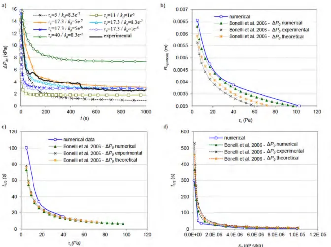
Figure 10a presents the results obtained for these different sets of parameters. The evolution of the pressure differential between location#3 and location#4 as a function of time is presented, in comparison with the experimental data. In accordance with the erosion law implemented in our interface displacement code, we observed that only the critical shear stress has an influence on the erosion figure at the end of the erosion process. Let us denote R! the radius of the erodible pipe of length L over time t!, for which the erosion process no longer evolves, t1/ 2 the time in which the radius of the pipe at x=6 cm equals:
( )
1/ 2 0(
0)
2R t =R + R!"R , g1 and g2 two continuous functions on ! . In agreement with the erosion law + Eq. (1), we verify that:
( )
1 cR! =g ! and t1/ 2 =g2
(
kd,!c)
(19)Figure 10b shows function g1, by plotting the final radius, taken at the middle of the channel, as a function of the critical shear stress. Figures 10c and 10d show function g2, by plotting t1/ 2 as a function of the critical shear stress and the erosion coefficient respectively. These results are compared to the analytical formulas of Bonelli et al. [2] : 1/ 4 5 0 0 2L c R P R ! ! " # $ =%% && ' ( ) (20) ! "
( )
( )
! ! 1/ 4 1/ 4 1/ 2 1/ 2 5/ 4 1 2 er c c c t t f ! R t f ! ! ! # $ " =) ' (% *& + , - . (21)It can be seen in Figures 10b, 10c and 10d that the numerical and analytical results agree well, whatever the pressure differential chosen for the analytical model at t=0 s. Figure 10b shows the curves staggered as a function of the initial pressure differential, but their shapes correspond well with that obtained numerically. Figures 10b and 10c show that the higher the stress threshold, the less pronounced the erosion of the soil, and the faster the erosion process occurs. Likewise, the higher the erosion coefficient, the faster the erosion process occurs (Figure 10d). The parametric study of the influence of the critical shear stress and the erosion kinetic coefficient also permits obtaining the amplitude of the consequences of errors on these two parameters. The lower the critical shear stress, the larger the errors generated will be on the erosion figure and on the erosion kinetics. These errors can intensively vary depending on the value of the critical shear stress and the erosion coefficient. For low erosion coefficients and threshold stresses, the curves related to the erosion kinetics present asymptotes. That is why the erosion kinetics is very sensitive to the variation of these parameters for these ranges of !c and kd. For a critical shear stress from 0 to 10 Pa, an error of several per cent can lead to an error higher than 100% over the period of the erosion process, which is also the case for kd <10!6 m .s/kg2 .
6.
Discussion
The first point to be discussed concerns the fact that we did not consider any transient flow regime in our numerical model. Indeed, the flow rate imposed at the inlet was constant throughout the test, which explains the errors observed on the initial pressure differential. The numerical results nonetheless remain close to the experimental results, thus omitting the transient phase appears to be a reasonable hypothesis, at least for these three tests.
The second element of discussion deals with the agreement between numerics, experiments and analytical model. For the Hole Erosion Test carried out on soil A, D and E, we observe that the erosion parameters found experimentally permit to model accurately the evolution of the erosion process. This represents an additional validation of the HET interpretation model and of the modelling method. The parametric studies performed also show the extent to which the erosion parameters found with the other test could lead to a considerable error between the numerical results and the experimental ones. From this, we can infer that the HET interpretation model is validated, at least for these soils. However, the physical meaning of the erosion parameters cannot be assessed with such numerical model.
Also, whatever the test considered, the erosion figures obtained numerically are very similar, as can be seen in Figure 6. However, the flatness of the water/soil interfaces presented in Figure 6 is never observed experimentally at the end of an HET. An erosion profile obtained experimentally presents several instabilities and fluctuations as underlined by Benahmed and Bonelli [1]. The instabilities usually observed in the pipe result from complex processes, surely dependent on the internal structure of the soil and would need further investigations.
Eventually, the range of the erosion parameters for which the numerical and analytical models are validated can also be discussed. Indeed, in addition to the validations performed on soil A, a good agreement is observed between the numerical and experimental results and those of the analytical model for the tests on soils D and E. The erosion parameters obtained make it possible to represent the evolution of the erosion process numerically, at least in terms of orders of magnitude. This provides another additional validation of the HET interpretation model and of the modelling method. Admittedly, the range of erosion parameters is not very wide, with critical shear stresses varying only from 6 to 26 Pa and erosion coefficients spread over an order of magnitude: from 1.38x10⁻⁷ to 1.71x10⁻⁶ m².s/kg, which corresponds to Fell’s indexes between 2 and 4. For HET experiments with real natural soils, the critical shear stress can reach 200 Pa and Fell’s index can vary from 0 to 8. Widening the range of erosion parameters of the test modelled could be one way of further investigation in the spirit of the present study.
7.
Conclusion
This study focuses on the numerical modelling of piping erosion of a cohesive soil by a turbulent flow in the specific configuration of the Hole Erosion Test. The numerical modelling method is based on an Euler-Lagrange resolution process. The flow is described by a Navier-Stokes turbulent model with mobile interface and remeshing. A Lagrangian method is developed for the moving frontier. The assumption of a diluted flow and cohesive soil allow considering that both the fluid and solid phases are monophasic. The hypothesis of slow erosion kinetics permits a decoupled sequential resolution. The numerical model is first validated for piping erosion due to a laminar flow in a 2-dimensional geometry with a constant pressure drop. The results agree very well with the analytical prediction [4], with a relative error of less than 2%. Then, regarding the piping erosion of cohesive soils by a turbulent flow, at constant flow rate, the numerical results are compared to the analytical model by Bonelli et al. [2], once again with good agreement for the asymptotic values and the erosion kinetics. A parametric study of the influence of the critical shear stress and the erosion coefficient is also conducted and confirmed that the characteristic duration of erosion depends on both parameters while the asymptotic radius is solely a function of the critical shear stress. The numerical modelling of two additional Hole Erosion Tests permits confirming the validation of the modelling method developed and comparing the results obtained for different erosion parameters and erosion kinetics. The good agreement between the numerical results, the experimental results and the analytical predictions shows that it is now possible to model the piping erosion of a cohesive soil by turbulent flow with good accuracy and within reasonable calculation times. This numerical model is able to reproduce accurately the erosion of a cohesive soil by a concentrated leak. It also gives access to a detailed description of all the averaged hydrodynamic flow quantities that are essential in order to achieve a better understanding of the erosion processes. The scope of this study was on the hydrodynamics which gives rise to erosion and for this reason the erosion resistance of the soil was assumed uniform and homogeneous. However, temporal evolution of the erosion resistance can arise from various degradation processes such as
swelling effects while spatial heterogeneities are likely within a real soil sample. Accounting for such time and space variabilities of the erosion resistance could be possibly integrated into our model as a next step.
8.
Acknowledgements
The authors are grateful to the Centre d’Ingénierie Hydraulique of EDF and geophyConsult for their financial support. They also extend special thanks to Mrs Patrick Pinettes (geophyConsult), Jean-Robert Courivaud (EDF) and Jean-Jacques Fry (EDF) for their support and confidence. This work was also funded by the French National Research Agency (ANR) through the COSINUS program (project CARPEINTER No. ANR-08-COSI-002).
9.
References
1. Benahmed N and Bonelli S (2012) Investigating concentrated leak erosion behaviour of cohesive soils by performing hole erosion tests. European Journal of Environmental and Civil Engineering 16(1):43-58
2. Bonelli S, Brivois O, Borghi R and Benahmed N (2006) On the modelling of piping erosion. Comptes Rendus de Mécanique 334(8-9):555-559
3. Bonelli S and Brivois O (2008) The scaling law in the hole erosion test with a constant pressure drop. International Journal for Numerical and Analytical Methods in Geomechanics 32:1573-1595
4. Bonelli S, Golay F, Mercier F (2012) Chapter 6 - On the modelling of interface erosion. In: Erosion of geomaterials, Wiley/ISTE
5. Brivois O, Bonelli S and Borghi R (2007) Soil erosion in the boundary layer flow along a slope : a theoretical study. European Journal of Mechanics /B Fluids 26:707-719
6. Chen HC and Patel VC (1988) Near-Wall Turbulence Models for Complex Flows Including Separation. AIAA Journal 26(6):641–648
7. Donea J, Guiliani S and Halleux JP (1982) An arbitrary lagrangian eulerian finite element method for transcient dynamics fluid structure interaction. Comp. Meth. Appl. Mech. Eng. 33:689-723
8. Golay F, Lachouette D, Bonelli S and Seppecher P (2010) Interfacial erosion: A three-dimensional numerical model. Comptes Rendus de Mécanique 338:333-337
9. Lachouette D, Golay F and Bonelli S (2008) One dimensionnal modelling of piping flow erosion. Comptes Rendus de Mécanique 336:731-736
10. Launder BE and Spalding DB (1972) Lectures in Mathematical Models of turbulence. Academic Press, London
11. Osher S and Sethian J (1981) Fronts propagating with curvature dependent speed: algorithm foot tracking material interface. Journal of Computational Physics 39:201-225
12. Ouriemi M, Aussillous P, Médale M, Peysson Y and Guazzelli E (2007) Determination of the critical Shields number for particle erosion in laminar flow. Physics of Fluids 19(6)
13. Pope SB (2000) Turbulent Flows. Cambridge University Press
14. Regazzoni P-L and Marot D (2011) Investigation of interface erosion rate by Jet Erosion Test and statistical analysis. European Journal of Environmental and Civil Engineering 15(8):1167-1185
15. Shih T-H, Liou WW, Shabbir A, Yang Z and Zhu J (1995) A New k-epsilon Eddy-Viscosity Model for High Reynolds Number Turbulent Flows - Model Development and Validation. Computers Fluids 24(3):227–238 16. Vardoulakis I, Stavropoulou M and Papanastasiou P (1996) Hydromechanical aspects of sand production problem. Transport in Porous Media 22:225-244
17. Wan CF and Fell R (2004) Laboratory Tests on the Rate of Piping Erosion of Soils in Embankment Dams. Journal of Geotechnical Testing Journal 27(3):295-303
18. Wolfshtein M (1969) The Velocity and Temperature Distribution of One-Dimensional Flow with Turbulence Augmentation and Pressure Gradient. Int. J. Heat Mass Transfer 12:301–318
Soil A Soil D Soil E Flow rate (m3/h) 0.531 0.546 0.236
Sample length (cm) 12 15 15
Critical shear stress τc (Pa) 17.3 25.8 6.35
Erosion coefficient kd (m².s/kg) 8.3.10-7 1.4.10-7 1.7.10-6
Table 1 Characteristics of the different meshes studied to investigate the influence of mesh density on the
numerical results
Soil A Soil D Soil E
Soil content Silt with
broken stones Clay (White kaolinite)
Mixture of 30% clay (proclay) and fine sand
(70%)
Water content (%) 16.2 23.5 21
Apparent density (t/m3) 1.83 1.39 1.66
Void ratio 0.48 0.9 0.60
Degree of saturation (%) 92 69.1 92.9
Clay plasticity index 11 16 24
% passing through 80 µm 51.4 90 94.9
Table 2 Identification parameters of soils A, D and E [1]
Mesh Mesh size on the water/soil
interface (cm) y + Total number of cells A 0.03 35.1 12 968 B 0.023 23.2 20 446 C 0.015 14.4 31 366 D 0.008 8.1 62 852 E 0.003 5.1 70 532 F 0.003 3.7 138 832 G 0.0019 2.2 400 326 H 0.0008 1.3 695 300
Table 3 Hydraulic and erosion parameters relating to the HET tests performed on soils A, D and E
Relative error on !P34 (%)
at the end of the erosion process Soil A Soil D Soil E In comparison to the experimental results 15.6 55.7 21.2
In comparison to the analytical model 18.2 13.1 30.2
Table 4 Relative errors on the pressure differential between location#3 and location#4, at the end of the erosion
Fig. 1 Simplified schematic diagram of the Hole Erosion Test
Fig. 2 Evolution of the pressure differential between sections A and B for tests of soils A, D and E, comparison
Fig. 3 Photographs of soil samples before (left) and after (right) HET tests, with from top to bottom images
corresponding to soils A, D and E respectively (F. Byron, IRSTEA)
Fig. 4 Independence of results relating to meshing density: a) average velocity on the axis of symmetry at zero
Fig. 5 Evolution velocity fields and the erosion trace as a function of time, modelling of the HET performed on
soil A
Fig. 6 Shape of the erosion traces obtained numerically, comparison of the results obtained for the test performed
Fig. 7 Evolution of a) the shear stress and b) the pressure field, on the water/soil interface, as a function of time
Fig. 8 Evolution of a) the shear stress for the three tests and b) the shear stress in case of soil A for the different
Fig. 10 Results of the parametric study: a) Evolution of the pressure differential between location#3 and
location#4 in comparison with experimental data, b) radius of the channel, at x=6 cm at the end of the erosion process, c) illustration of the erosion kinetics as a function of the critical shear stress and d) illustration of the erosion kinetics as a function of the erosion coefficient, in comparison with the results given by the model of Bonelli et al. [2], for the different ∆P0