HAL Id: tel-01425642
https://tel.archives-ouvertes.fr/tel-01425642v2
Submitted on 12 Oct 2017HAL is a multi-disciplinary open access
archive for the deposit and dissemination of sci-entific research documents, whether they are pub-lished or not. The documents may come from teaching and research institutions in France or abroad, or from public or private research centers.
L’archive ouverte pluridisciplinaire HAL, est destinée au dépôt et à la diffusion de documents scientifiques de niveau recherche, publiés ou non, émanant des établissements d’enseignement et de recherche français ou étrangers, des laboratoires publics ou privés.
to fixed-point conversion targeting embedded processors
Ali Hassan El Moussawi
To cite this version:
Ali Hassan El Moussawi. SIMD-aware word length optimization for floating-point to fixed-point conversion targeting embedded processors. Computer Arithmetic. Université Rennes 1, 2016. English. �NNT : 2016REN1S150�. �tel-01425642v2�
ANNÉE 2017
THÈSE / UNIVERSITÉ DE RENNES 1
sous le sceau de l’Université Bretagne Loire
pour le grade de
DOCTEUR DE L’UNIVERSITÉ DE RENNES 1
Mention : Informatique
Ecole doctorale Matisse
présentée par
Ali Hassan El Moussawi
Préparée à l’Unité Mixte de Recherche 6074 – IRISA
Institut de recherche en informatique et systèmes aléatoires
UFR Informatique Electronique
SIMD-aware Word
Length
Optimiza-tion
for
Floating-point to Fixed-Floating-point
Conversion
targe-ting Embedded
Pro-cessors
Thèse soutenue à Rennes le 16/12/2016
devant le jury composé de :
David Defour
MCF - Université de Perpignan / Rapporteur
Lionel Lacassagne
PR - Université Pierre et Marie Curie / Rapporteur
Karine Heydemann
MCF - Université Pierre et Marie Curie / Examina-trice
Daniel Menard
PR - INSA Rennes / Examinateur
Tomofumi Yuki
CR - INRIA Bretagne Atlantique / Examinateur
Steven Derrien
Certes, la science guide, dirige et sauve; l’ignorance égare, trompe et ruine.
Remerciements
Steven a toujours été là pour me conseiller et me motiver, je tiens à le remercier infiniment pour tout ce qu’il a fait pour contribuer à la réussite de mes travaux de thèse.
Je remercie d’autant Tomofumi Yuki pour le temps qu’il a consacré pour discuter des divers aspects de cette thèse. Ses conseils avaient un impact important sur ces travaux.
Je tiens également à remercier Patrice Quinton pour sa contribution à la revue/correction de ce manuscrit.
Je remercie tous les membres du jury, qui m’ont fait l’honneur en acceptant de juger mes travaux, surtout Lionel Lacassagne et David Defour qui ont eu la charge de rapporteurs.
Je remercie tout le personnel de l’Inria/Irisa, notamment les membres de l’équipe CAIRN pour le chaleureux accueil qu’ils m’ont réservé. Je remercie, en particulier, Nadia Derouault qui s’est occupée de toutes les démarches administratives, Nicolas Simon et Antoine Morvan pour l’assistance avec les outils de développement, ainsi que Gaël Deest, Simon Rokicki, Baptiste Roux et tous les autres.
Table of Contents
Résumé en Français v List of Figures xi List of Tables xv Glossary xvii 1 Introduction 11.1 Context and Motivations . . . 2
1.2 ALMA Project . . . 4
1.3 Timeline . . . 6
1.4 Contributions and Organization . . . 8
2 Background: Floating-point to Fixed-point Conversion 11 2.1 Introduction . . . 12
2.2 Floating-point Representation . . . 12
2.3 Fixed-point Representation . . . 14
2.4 Floating-point vs. Fixed-point . . . 16
2.5 Floating-point to Fixed-point Conversion Methodologies . . . 19
2.5.1 Integer Word Length Determination . . . 19
2.5.2 Word Length Optimization . . . 21
2.5.3 Fixed-point Code Generation . . . 22
2.6 Automatic Conversion Tools . . . 23
2.6.1 Matlab Fixed-point Converter . . . 23
2.6.2 IDFix . . . . 24
2.7 Conclusion . . . 27
3 Background: Single Instruction Multiple Data 29 3.1 Introduction . . . 30
3.2 SIMD Instruction Sets . . . 31
3.2.1 Conventional Vector Processors . . . 31
3.2.2 Multimedia extensions . . . 32 i
3.3 Exploiting Multimedia extensions . . . 36
3.3.1 Manual Simdization . . . 37
3.3.2 Automatic Simdization Methodologies . . . 38
3.4 Conclusion . . . 42
4 Superword Level Parallelism 45 4.1 Introduction . . . 46
4.2 Related work . . . 47
4.2.1 Original SLP. . . 48
4.2.2 Original SLPExtensions and Enhancements . . . 49
4.3 Holistic SLP . . . 50
4.3.1 Overview . . . 51
4.3.2 Shortcomings . . . 59
4.4 Proposed Holistic SLP Algorithm Enhancements . . . 64
4.4.1 Pack Flow and Conflict Graph (PFCG) . . . 65
4.4.2 Group Selection Procedure . . . 66
4.4.3 Algorithm complexity . . . 72
4.4.4 Pseudo-code . . . 74
4.5 Experimental Setup and Results . . . 78
4.5.1 Implementation . . . 78 4.5.2 Target processors . . . 79 4.5.3 Benchmarks . . . 81 4.5.4 Tests Setup . . . 81 4.5.5 Results . . . 82 4.6 Conclusion . . . 88
5 SLP-aware Word Length Optimization 91 5.1 Introduction . . . 92
5.2 Motivations and Related Work . . . 94
5.3 Joint WLO and SLP extraction . . . 96
5.3.1 Overview and Intuition . . . 97
5.3.2 Processor Model . . . 98
5.3.3 SLP-aware WLO algorithm . . . 101
5.3.4 Accuracy-aware SLP extraction algorithm . . . 106
5.3.5 SLP-aware Scalings Optimization . . . 109
5.4 Source-to-source Compilation Flow . . . 112
5.4.1 Flow Overview . . . 112
5.4.2 Integer Word Length determination . . . 114
5.4.3 Accuracy evaluation . . . 115
5.4.4 Select and sort Basic-blocks for SLP . . . 115
5.4.5 Fixed-point/SIMD Code Generation . . . 115
TABLE OF CONTENTS iii
5.5.1 Experimental Setup . . . 116
5.5.2 WLO-then-SLPsource-to-source flow . . . 117
5.5.3 Benchmarks . . . 118 5.5.4 Target Processors . . . 119 5.5.5 Results . . . 119 5.5.6 Floating-point vs. Fixed-point . . . 121 5.5.7 WLO+SLP vs. WLO-then-SLP . . . 121 5.6 Conclusion . . . 123 6 Conclusion 125 A Target Processor Models 129 A.1 XENTIUM . . . 129 A.2 ST240 . . . 129 A.3 KAHRISMA . . . 130 A.4 VEX . . . 130 Publications 133 Bibliography 135
Résumé en Français
Les processeurs embarqués sont soumis à des contraintes strictes de coût, consommation électrique et performance. Afin de limiter leur coût et/ou leur consommation électrique, certain processeurs ne disposent pas de support matériel pour l’arithmétique à virgule flottante.
D’autre part, les applications dans plusieurs domaines, tel que le traitement de signal et la télécommunication, sont généralement spécifiées en utilisant l’arithmétique à virgule flottante, pour des raisons de simplicité. Cette implémentation prototype est ensuite adaptée/optimisée en fonction de l’architecture cible.
Porter de telles applications sur des processeurs embarqués sans support matériel pour l’arithmétique à virgule flottante, nécessite une émulation logicielle, qui peut sévèrement dé-grader les performances de l’application. Pour éviter cela, l’application est convertie pour utiliser l’arithmétique à virgule fixe, qui a l’avantage d’être plus efficace à implémenter sur des unités de calcul entier. Les deux representations, à virgule flottante et à virgule fixe sont illustrées dans la fig. 1. La conversion de virgule flottante en virgule fixe est une procédure délicate qui implique
I F i f LSB s W E 1 M s e m LSB
partie entière partie fractionnelle exposant mantisse
virgule (implicite)
Nombre representé: sif * 2-F (-1)s * mantisse * 2exposant
Figure 1 – Comparaison des representations à virgule flottante (droite) et à virgule fixe (gauche). des compromis subtils entre performance et précision de calcul. Elle permet, entre autre, de réduire la taille des données au prix d’une dégradation de la précision de calcul. En effet, utiliser des opérations à virgule fixe, tout en gardant la précision complète des résultats, nécessite une augmentation considérable des tailles de mots des données. Par exemple, le résultat exact d’une multiplication entre deux nombres de taille w, nécessite une taille de 2w. Cette augmentation de la taille de mots peut dépasser la taille maximale supportée par le processeur cible, nécessitant ainsi une émulation logicielle d’opérateurs de taille plus grande, qui peut aussi bien dégrader la performance de l’application. Afin d’éviter cela, les tailles des données (et des résultats des opérations) sont réduites en appliquant des quantifications, qui correspondent à éliminer les bits de poids faibles. Ces opérations de quantification introduisent des erreurs de calcul, appelées
erreurs de quantifications, qui se propagent dans le système et peut engendrer une erreur impor-tante en sortie, dégradant ainsi la précision du résultat. En règle générale, plus la quantification est grande (i.e. plus la taille des données est réduite), plus la précision est faible mais meilleur est la performance. Il existe donc un compromis entre précision de calcule et performance.
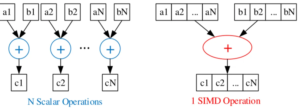
Par ailleurs, la plupart des processeurs embarquées fournissent un support pour le calcul vectoriel de type SIMD ("Single Instruction Multiple Data") afin d’améliorer la performance. En effet, cela permet l’exécution d’une opération sur plusieurs données simultanément, réduisant ainsi le temps d’exécution. Cependant, il est généralement nécessaire de transformer l’application pour exploiter les unités de calcul vectoriel. Cette transformation de vectorisation est sensible à la taille des données; plus leurs tailles diminuent, plus le taux de vectorisation augmente. Il apparaît donc un autre compromis entre vectorisation et tailles de données.
En revanche, la vectorisation ne conduit toujours pas a une amélioration de performance, elle peut même la dégrader ! En fait, afin d’appliquer une opération vectorielle, il faut d’abord agréger ou compacter les données de chacun des opérandes pour former un vecteur, qui correspond en générale à un registre SIMD. De même, il faut décompacter les données afin de les utiliser séparément, comme le montre la fig. 2. Ces opérations de (dé)compactage peuvent engendrer
aN ... a2 a1 b1 b2 ... bN
+
cN ... c2 c1+
a1 b1 c1+
a2 b2 c2+
aN bN cN...
Compacté en Registre SIMD compacter compacter ... Vectorisation décompacter En mémoire ... a1 a2 aN ... cN ... c2 c1Figure 2 – Illustration de la transformation de vectorisation remplacant N opérations scalaires par une seule opération SIMD plus les opérations de (dé)compactage.
un surcoût important dans le cas où les données sont mal organisées en mémoire. Du coup, afin d’améliorer efficacement la performance, la transformation de vectorisation doit prendre en considération ce surcoût.
La conversion de virgule flottante en virgule fixe et la vectorisation sont deux transformations délicates qui nécessitent un temps de développement très élevé. Pour remédier à ça et réduire les délais de mise sur le marché des applications, une multitude de travaux ont ciblé l’automatisation
vii
(complète ou partielle) de ces transformations. Dans l’état de l’art, on trouve des méthodolo-gies permettant la conversion de virgule flottante en virgule fixe, tel que [51, 26, 64, 85]. Ces méthodologies comportent en générale trois parties principales :
— La détermination des tailles des parties entières. En se basant soit sur des simulations, ou en utilisant des méthodes analytiques telle que l’arithmétique d’intervalles et l’arithmétique affine.
— La détermination des tailles des mots. Cela fait en générale l’objet d’une optimisation exploitant le compromis entre précision et performance, connue sous le nom "Word Length Optimization" ou WLO (optimisation de taille de mots). Pour ce faire, des méthodes permettant l’estimation de la précision de calcule et la performance, d’une implémentation à virgule fixe, sont nécessaires. Plusieurs méthodes ont été proposées.
— La génération de code à virgule fixe [50].
D’autre part, on trouve également des méthodologies permettant l’exploitation des unités de calcul SIMD, entre autre, les techniques d’extractions du parallélisme au niveau du bloque de base, connues sous le nom "Superword Level Parallelism" ou SLP (Parallélisme au niveau du super-mot) introduit en 2000 par Larsen et Amarasinghe [69]. Ces méthodes ont pour ob-jectif de trouver des groupes d’opérations, dans un bloque de base, qui peuvent être replacer par des opérations SIMD. Un tel groupe, appelée groupe SIMD, doit contenir des opérations, indépendantes, du même type (addition, multiplication, . . . ) et traitant des données de même taille. Le but des algorithmes d’extraction du SLP [69, 125, 78] est de trouver la « meilleure » solution de groupage qui permet d’améliorer la performance en tenant en compte le surcoût lié aux opérations de (dé)compactage.
Cependant, dans l’état de l’art, ces deux transformations sont considérées indépendamment, pourtant elles sont fortement liées. En effet, WLO détermine la taille des données qui affectent directement l’espace de recherche du SLP, et par conséquence la performance de la solution trouvée. Si WLO n’est pas conscient des contraintes d’extraction du SLP et du surcoût associé, il sera incapable d’estimer correctement l’impacte de ces décisions sur la performance finale de l’application (après avoir appliquer la conversion en virgule fixe et l’extraction du SLP). Par con-séquence, il sera incapable d’exploiter efficacement le compromis enter précision et performance. Afin de mieux exploiter ce compromis, WLO doit prendre en considération SLP, alors que ce dernier ne peut pas procéder sans avoir une connaissance sur les tailles des données. Ce problème d’ordonnancement de phase est illustré par la fig. 3.
SLP WLO
SIMD Groups
Word-lenghts
Dans ce contexte, on propose dans un premier temps un algorithme amélioré pour l’extraction du SLP. On se base sur un algorithme de l’état de l’art proposé en 2012 par Liu et al, on l’analyse soigneusement pour déterminer ses faiblesses puis on propose des améliorations pour y remédier. L’algorithme proposée est ensuite implémenté dans une plateforme de compilation source-à-source, Generic Compiler Suite (Gecos)[38], ainsi que l’algorithme de référence, afin de valider notre approche. Les résultats expérimentaux, extraits sur un ensemble de neuf applications de tests et ciblant plusieurs processeurs embarqués, montrent une amélioration claire apportée par notre algorithme.
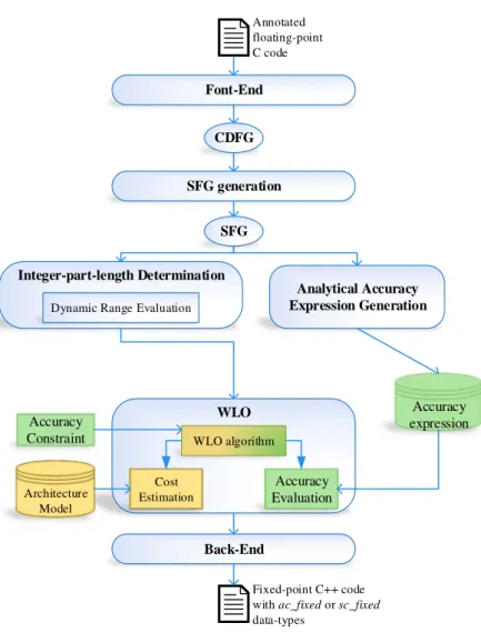
Ensuite, on propose une nouvelle technique permettant l’application conjointe, de la conver-sion de virgule flottante en virgule fixe et de l’extraction du SLP. Au contraire des méthodologies de l’état de l’art, cette nouvelle technique permet de mieux exploiter le compromis entre la pré-cision de calcul et la performance d’une application, ciblant des processeurs embarqués avec jeux d’instructions SIMD sans support matérielle pour l’arithmétique à virgule flottante. Cette ap-proche consiste à combiner un algorithme d’extraction du SLP conscient de la précision de calcul, avec un algorithme de WLO conscient des opportunistes de groupage SLP et du surcoût associé. Pour résoudre le problème d’ordonnancement de phases présenté précédemment, on a adapté l’algorithme d‘extraction du SLP proposé, afin de relâcher les contraintes liées à la tailles des données. De cette façon, l’extraction du SLP peut désormais démarrer sans avoir à attendre le résultat du WLO. l’algorithme d‘extraction du SLP est également conscient de la contrainte sur la précision de calcul, imposée par l’utilisateur. Cela permet d’éviter de sélectionner des groupes SIMD qui sont pas réalisable sans violer la contrainte de précision. Les groupes SIMD choisis, sont ensuite utilisés pour "guider" la sélection des tailles de mots par l’algorithme de WLO. La fig. 4 illustre cette approche. On implémente cette approche dans Gecos sous forme d’un flot
Accuracy-aware SLP extraction SLP-aware Scalings optimization Fixed-point Specification (IWLs only) SIMD Groups Fixed-point Specification (Complete) Basic blocks Accuracy Evaluation Service Processor Model Accuracy Constraint SLP-aware WLO groups WLs
Figure 4 – Illustration de l’approche proposée.
ix
approche, on la compare contre une approche classique appliquant indépendamment, d’abord la conversion de virgule flottante en virgule fixe, ensuite l’extraction du SLP, qu’on implémente également dansGecos. On teste les deux flots sur plusieurs processeurs embarquées. Les résul-tats confirme l’efficacité de notre approche, dans l’exploitation du compromis entre performance et précision.
List of Figures
1 Comparaison des representations à virgule flottante (droite) et à virgule fixe
(gauche). . . v
2 Illustration de la transformation de vectorisation remplacant N opérations scalaires par une seule opération SIMD plus les opérations de (dé)compactage. . . vi
3 Problème d’ordonnancement de phase entre WLO et SLP. . . vii
4 Illustration de l’approche proposée. . . viii
1.1 CPU trend over the last 40 years. Published by K. Rupp at www.karlrupp.net/ 2015/06/40-years-of-microprocessor-trend-data . . . 2
1.2 ALMA tool-chain flow diagram. . . 5
1.3 Outline. . . 9
2.1 Binary representation of floating-point numbers in IEEE 754 standard. . . 12
2.2 Binary representation of a signed fixed-point number. . . 14
2.3 IEEE single-precision floating-point numbers precision vs. range. . . 17
2.4 Range propagation example. . . 20
2.5 IDFix flow diagram. . . 25
3.1 Illustration of an Single Instruction Multiple Data (SIMD)addition operation in contrast to scalar addition operation. . . 30
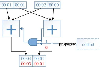
3.2 Illustration of Sub-word Level Parallelism (SWP) addition operator capable of executing 32-bit scalar addition (when propagate is 1) or 2x16-bitSIMDadditions (when propagate is 0). . . 34
3.3 Illustration of some soft SIMDoperations. . . 35
3.4 Example of Vectorization. . . 39
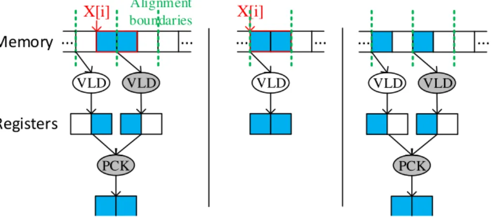
3.5 Illustration of vector memory load from an aligned stride-1 reference (middle) versus unaligned stride-1 (left) and aligned stride-2 (right), in case of a Multimedia extension with no support for unaligned accesses and with vector size of 2. . . 40
3.6 Example illustrating the difference between loop vectorization and Superword Level Parallelism (SLP). [min : max] represents a vector memory access to con-secutive array elements starting at offset min till offset max included. < a, b > represents a packing/unpacking operation. . . 42
4.1 Example C code snippet (left) and its statements dependence graph (right). . . 47 4.2 Recall example of fig. 4.1. . . 51 4.3 Holistic SLP algorithm flow diagram. . . 52 4.4 Variable Pack Conflict Graph (VPCG)andStatement Grouping Graph (SGG) of
the example in fig. 4.1. . . 53 4.5 AG({S4, S5}) at the first selection iteration of the example of fig. 4.1. . . 56 4.6 Updated VPCG (left) and SGG (right) after the selection of {S4, S5} of the
example of fig. 4.1. . . 57 4.7 Example illustrating holistic SLP algorithm. It shows that VPCGandSGGdo
not represent cyclic dependency conflicts. The grouping solution is {c1, c2, c3} which is not legal due to cyclic dependency between c1, c2 and c3. . . 60 4.8 Example showing how fake dependencies affect holistic SLP VP reuse estimation. 61 4.9 Example illustrating holistic SLP candidate benefit estimation. . . 63 4.10 SLP extraction framework overview. . . 65 4.11 Data Flow Graph (DFG) and Pack Flow and Conflict Graph (PFCG) of the
ex-ample in fig. 4.1. Rectangular nodes in thePFCGrepresent pack nodes, whereas elliptic shaped ones represent candidate nodes. Undirected edges represent con-flicts between candidates and directed edges represent Variable Pack (VP) Flow. Highlighted nodes (with orange) indicate a reuse. . . 67 4.12 Execution time improvement, over the sequential version, of various benchmarks
obtained by applying holistic SLP for ten times. . . 69 4.13 Execution time improvement, over the sequential version, of various benchmarks
after applying the proposedSLP extraction for ten times. . . 70 4.14 Recall the example of fig. 4.9. . . 71 4.15 PFCGof the example in fig. 4.14 at the first iteration using prop-2. . . 71 4.16 Execution time improvement of the SIMD code obtained by applying our
pro-posed SLP extraction method, compared to the original (sequential) code, for different values of N considered for constructing the distance-N neighborhood of a candidate (sub-PFCG) in thePFCG. The targeted processor is KAHRISMA. . 73 4.17 SLP Extraction Framework implementation inGecos. . . 79 4.18 Test procedure diagram. . . 82 4.19 Execution time improvement of the SIMD code obtained by prop vs. hslp, over
orig. The test is repeated 10 times for each benchmark. A bar represent the mean value and a line segment represents the minimum and maximum values of the execution time improvement. . . 84 4.20 Execution time improvement of the SIMD code obtained by prop vs. hslp, over
orig. The test is repeated 10 times for each benchmark. A bar represent the mean value and a line segment represents the minimum and maximum values of the execution time improvement. . . 85 4.21 Using prop. . . 87 4.22 Execution time improvement and Simdization time variation with respect to the
LIST OF FIGURES xiii
5.1 C code snippet. . . 93
5.2 Motivating example. . . 96
5.3 WLO/SLP phase ordering problem. . . 97
5.4 Overview of the joint Word Length Optimization (WLO) and SLP extraction approach . . . 98
5.5 Fixed-point multiplication example. . . 100
5.6 Fixed-point multiplication example. . . 101
5.7 Representation of an operation node (op) and its predecessors/successor data nodes (dx) in a fixed-point specification. < ix, fx> represents a fixed-point format with ix representing the Integer Word Length (IWL)and fx theFractional Word Length (FWL). Elliptical nodes represent scaling operations; a negative amount corresponds to a left shift by the absolute value. . . 103
5.8 Scaling example. fx represents the FWL. . . 111
5.9 SLP-aware WLO source-to-source compilation flow diagram. . . 113
5.10 Test setup . . . 117
5.11 WLO-then-SLP source-to-source compilation flow diagram. . . 118
5.12 Speedup ofSIMDcode version obtained by WLO+SLP flow, over the original float version, for different accuracy constraints expressed in dB (higher values (to the left) are less accurate) . . . 120
5.13 Speedup (higher is better) comparison between SIMD versions of WLO-then-SLP and WLO+SLP vs. accuracy constraint expressed in dB (higher values(to the left) are less accurate). The baseline is the execution time of the (nonSIMDfixed-point version of WLO-then-SLP. . . 122
List of Tables
2.1 Exact fixed-point operations. . . 15 2.2 Floating-point vs. Fixed-point. . . 19 4.1 Test Benchmarks. . . 81 4.2 Number of operations and memory accesses in benchmarks. CAA represents the
number of contiguous array access candidates. . . 81 5.1 Benchmarks . . . 118 5.2 Target processors supported operations. . . 120 A.1 XENTIUM Model. . . 129 A.2 ST240 Model. . . 130 A.3 KAHRISMA Model. . . 130 A.4 VEX Model. . . 131
Glossary
API Application Programming Interface. DAG Directed Acyclic Graph.
DFG Data Flow Graph. DLP Data Level Parallelism. DSP Digital Signal Processor. FWL Fractional Word Length. Gecos Generic Compiler Suite. HLS High-Level Synthesis. HP Hawlett-Packard. IR Intermediate Representation. ISA Instruction Set Architecture. IWL Integer Word Length.
KIT Karlsruhe Institute of Technology. LSB Least Significant Bit.
LTI Linear Time-Invariant. MIS Multimedia Instruction Set. MMX Matrix Math eXtension. MSB Most Significant Bit.
PFCG Pack Flow and Conflict Graph.
SCoP A loop nest in which all loop bounds, conditionals and array subscripts are affine functions of the surrounding loop iterators and parameters.
SFG Signal Flow Graph.
SGG Statement Grouping Graph. SIMD Single Instruction Multiple Data.
Simdization The process of converting scalar instructions in a program into equivalentSIMD instructions.
SLP Superword Level Parallelism.
SQNR Signal-to-Quantization-Noise Ratio. SWP Sub-word Level Parallelism.
TI Texas Instruments.
VLIW Very Long Instruction Word. VP Variable Pack.
VPCG Variable Pack Conflict Graph. WLO Word Length Optimization.
Chapter 1
Introduction
Contents
1.1 Context and Motivations . . . 2 1.2 ALMA Project . . . 4 1.3 Timeline . . . 6 1.4 Contributions and Organization . . . 8
100 101 102 103 104 105 106 107 1970 1980 1990 2000 2010 2020 Year Number of Logical Cores Frequency (MHz) Single-Thread Performance (SpecINT x 103) Transistors (thousands) Typical Power (Watts)
Original data up to the year 2010 collected and plotted by M. Horowitz, F. Labonte, O. Shacham, K. Olukotun, L. Hammond, and C. Batten New plot and data collected for 2010-2015 by K. Rupp
Figure 1.1 – CPU trend over the last 40 years. Published by K. Rupp at www.karlrupp.net/2015/ 06/40-years-of-microprocessor-trend-data
1.1 Context and Motivations
Ever since the first transistor computers appeared in the late ’50s, manufacturing technologies kept continuously improving, allowing a steady exponential growth of the transistor count that can be integrated into a single die. This improvement rate was early observed by Gordon Moore in the mid ’60s, when he predicted that the transistor density in an integrated circuit would double every two years. This has later led to the famously known Moore’s law.
The transistor density growth, up to the early 2000s, was mostly invested in improving single core CPU performance, as shown in the graph of fig. 1.1. This was essentially achieved by increas-ing the core operational frequency, up to a point where the power density became too high for the generated heat to be practically dissipated. Limited by this Power Wall, frequency increase has stalled (mid 2000s) while the transistor density kept on increasing exponentially, causing a shift in focus toward multi-core parallelism. Though, other forms of (intra-core) parallelism have been exploited since the ’60s, including pipelining, superscalar execution and Single In-struction Multiple Data (SIMD), which contribute to the continuous improvement of single-core performance.
Unlike general purpose (mainstream) processors, embedded ones are subject to stricter design constraints including performance, cost and power consumption. Indeed, they are destined to be
Context and Motivations 3
used in a wide variety of domain-specific applications with, for instance, a limited power source. In many application domains, such as signal processing and telecommunication, real numbers computation is employed. Since exact real numbers are not practically possible to represent in a processor, designers/developers resort to alternative, approximative representations of real numbers, which should be accurate enough while satisfying performance, power consumption and cost constraints of the targeted application. Among the most commonly used such repre-sentations are floating-point and fixed-point. Floating-point representation has the advantage to be very easy to use but it requires dedicated hardware support which increase the cost. On the other hand, fixed-point is cheaper since it is based on integer arithmetic but it is more complex to use, which increase the development time. So, the choice between these possibilities is mainly a tradeoff between cost (and power consumption) and ease of programmability.
Many embedded processors nowadays, such the ARM cortex-A family, provide hardware sup-port for floating-point arithmetic, however a good number of ultra low power embedded proces-sors, such as ARM cortex-M0/1/3, TI TMS320 C64x and Recore XENTIUM, do not. This comes at the cost of restraining programmability to the use of fixed-point arithmetic, while application prototyping generally employs floating-point the for sake of simplicity. This means that imple-menting the application on such processors requires either a software emulation of floating-point arithmetic or a conversion of floating-point into fixed-point. While feasible, software emulation of floating-point results in very poor performance. Alternatively, fixed-point implementation, if specified carefully, can achieve much (1 to 2 order of magnitude) better performance. However, this cannot always be done while keeping the same numerical accuracy, as it would require the use of increasingly large word-lengths, which unless supported by the target processor would also require software emulation, thus compromising performance. Instead, quantizations are applied to limit word-length growth at the cost of introducing quantization errors which alter the com-putation accuracy. This performance/accuracy tradeoff can be exploited during floating-point to fixed-point conversion in a process known asWord Length Optimization (WLO).
When targeting a processor that can only operate on data with a fixed word-length (the word-size, 32-bit in general),WLO does not make much sense. In fact, employing smaller data sizes does not necessarily benefit the application performance. On the one hand, it may require additional operations to perform data-type conversions, since all integer operations will eventually be performed on operands converted to the native word-size anyway. But on the other hand, it may reduce the memory footprint, which can improve performance. All in all, it is generally better to use the native word-size when targeting such processors.
The story changes when targeting processors with support forSIMD operations. In this case, smaller data word-lengths can be exploited to perform an operation on several (packed) data simultaneously, usingSIMD instructions. In principle at least, this helps reducing the number of operations, thus ultimately improving performance. This can be exploited during WLO to explore the performance/accuracy tradeoff. Most embedded processors, such as XENTIUM and ARMv7, provide support for SIMD with various levels. However, taking advantage of SIMD capabilities to improve performance is a challenging task.
Automated methodologies for floating-point to fixed-point conversion and Simdization1
are essential to reduce development cost and cut down time-to-market. None of the existing work tackles both transformations simultaneously, despite the strong relation between them. Typically, the floating-point to fixed-point conversion is performed first and thenSimdizationis (optionally) applied on the resulting fixed-point code.
In this thesis, we argue that considering both transformations independently yields less efficient solutions. We propose a new methodology to combine WLOwithSimdization.
1.2 ALMA Project
From a broader perspective, this thesis took place in the context of the European project ALMA[2]. As we mentioned previously, applications in many domains, such as signal processing, are prototyped or specified using floating-point arithmetic and without too much worry about the target architecture characteristics, such as parallelism, for the sake of simplicity. More often than not, the application prototyping is done using high-level numerical languages or frameworks such as Matlab or Scilab. Once the specification is ready, the implementation phase aims at providing an accurate and optimized implementation for the target architecture. In the case of embedded multi-core processors with no hardware support for floating-point arithmetic, this generally involves three main steps:
— Matlab (or Scilab) to C/C++ conversion. — Floating-point to fixed-point conversion. — Coarse and fine -grained Parallelization.
Each of these steps is time consuming and error prone, which greatly increases the development time.
To address this problem, MathWorks provides an automatic C code generator, from a subset of the Matlab language. However, the generated C code uses library calls to Matlab special functions, for which the source code is not provided. This makes the code difficult to optimize in a later stage. Besides, MathWorks tools are proprietary and open source alternatives, like Scilab, do not provide a similar functionality. Hence, the main motivations behind the ALMA project is to provide an alternative solution to this problem.
The ALMA project [2] aims at addressing the aforementioned problems by providing a com-plete tool-chain targeting embedded multi-core systems. An overview of the proposed tool-chain flow is depicted in fig. 1.2.
Starting from a Scilab code, the tool aims, in a first place, at automatically converting it into an annotated C code. The latter then undergoes a multitude of optimizations, mainly performing:
— Coarse-grain parallelization: to exploit the multi-core nature of the target processors.
ALMA Project 5
Figure 1.2 – ALMA tool-chain flow diagram.
— Floating-point to fixed-point conversion: to avoid performance degradation due to floating-point simulation.
— Simdization: to take advantage of theSIMD capabilities of the target processor cores. The tool finally generates a parallel C code using a generic MPI (message passing interface), SIMDand fixed-point Application Programming Interfaces (APIs).
ALMA targeted two multi-core architectures from Recore Systems and Karlsruhe In-stitute of Technology (KIT), based on the XENTIUM [104] and KAHRISMA [58] cores respectively. None of which support floating-point arithmetic, but they provide subword SIMD capabilities.
1.3 Timeline
In this section, we present a brief timeline of the work done during this thesis, in order to help understanding the context, choices and contributions made during this work.
In the context of ALMA, we mainly had to:
— Implement a floating-point to fixed-point conversion, since both ALMA targets do not provide hardware support for floating-point arithmetic2
.
— Implement an automatic Simdization, since compilers of ALMA targets do not perform this transformation.
— Explore the performance/accuracy tradeoff using WLO and taking into account SIMD opportunities.
So, we explored the state-of-the-art for floating-point to fixed-point conversion targeting embed-ded processors (cf. chapter 2). We found that most approaches are similar in the way they address the problem:
1. First, the Integer Word Lengths (IWLs) are determined based on dynamic range values, which can be obtained using simulation or analytical methods.
2. Then, the word-lengths are specified, either by simply using a default word-length (generally the native word-size e.g. 32-bit), or by performing a WLOunder and accuracy constraint. The different approaches differ in the way dynamic ranges are obtained and/or the WLO algo-rithm and/or the accuracy estimation procedure.
Integrating such transformations into the target compilers is not a trivial task, but most im-portantly it should be done for each different target to be supported by the flow. Instead, we decided to implement this conversion at source code level using a source-to-source compiler flow. For this matter, we used the source-to-source compilation framework, Generic Compiler Suite (Gecos)[38], which already integrates a floating-point to fixed-point conversion tool, IDFix [3], providing automatic dynamic range and analytical accuracy evaluation methods. Besides, this choice is also motivated by the fact that Gecos/IDFix provides an extension mechanism allow-ing for "simple" integration of different methods for range evaluation and accuracy estimation without affecting our work. However, IDFix was initially designed for targeting High-Level Synthesis (HLS) using C++ fixed-point libraries. Since not all embedded processor compilers support C++ and in order to avoid the performance overhead introduced by using such libraries, we implemented a fixed-point C code generator using native integer data-types and operations.
Timeline 7
Similarly, we decided to implement Simdization at source code level so that it can be easier to extend in order to support other targets. We investigated the different ways of performing Simdization. The existing techniques can be categorized into two groups:
— Loop-level vectorization.
— Basic-block level, also known asSuperword Level Parallelism (SLP).
We decided to go with SLP, since it can exploit more opportunities than loop vectorization without the need for "complex" dependency analysis and loop transformations. We investigated the state-of-the-art of SLP extraction algorithms and we decided to implement the algorithm proposed by Liu et al [78] in 2012. However, during the implementation we found many short-comings, so we came up with an improvedSLPextraction algorithm, that we present in chapter 4. We implemented it in addition to the aforementioned algorithm by Liu et al, so that we can compare them. We integrated theSLPextraction algorithms as well as aSIMDC code generator into the same source-to-source compilation framework,Gecos.
At this point, we had at our disposal a complete source-to-source flow capable of automatically generating a fixed-point SIMD C code for different embedded processors. With all that out of the way, we started exploiting the interaction between WLO on the one side and SLP on the other. In the literature, few existing floating-point to fixed-point conversion approaches target embedded processors with SIMD capabilities. Existing work though, do not consider Simdiza-tion while performing WLO; they simply assume that selecting narrower word-lengths would eventually increase the SIMD opportunities, and improve performance consequently. However, this assumption is very optimistic since theWLOin unaware of theSIMDopportunities and the associated cost overhead, which can result in a very high performance degradation3.
Using the source-to-source compilation flow we already implemented, we integrated a typ-ical WLO strategy that aims essentially at reducing data word-lengths without considering Simdization. In order to test how well such strategy can perform, we applied floating-point to fixed-point conversion (using the aforementionedWLOstrategy), followed by SLPextraction, on some benchmarks for XENTIUM, KAHRISMA and two other embedded processors. The results showed that such an approach is not very efficient for targeting SIMD processors; the observed speedup due toSimdizationvaries inconsistently, supporting our hypothesis about the fact that, simply minimizing word-lengths without taking into account theSimdizationproblem would yield inefficient solutions.
In order to solve this problem, we propose a new SIMD-aware floating-point to fixed-point conversion approach based on a joint WLO and SLP extraction algorithm. We also integrate the proposed joint WLO and SLP algorithm to the source-to-source compilation flow in order to test it validity compared to prior typical approach. Using our approach, we obtain more efficient overall solutions; it enables a better exploitation of the performance/accuracy tradeoff when targeting embedded processors.
1.4 Contributions and Organization
More specifically the contributions of this work are the following ones:
— A new Intermediate Representation (IR) for SLPextraction (cf. chapter 4). — A new SLP extraction algorithm (cf. chapter 4).
— A new approach for floating-point to fixed-point conversion considering, jointly, WLOand SLP extraction (cf. chapter 5).
— A fully automated source-to-source compilation flow4
for SLP extraction and floating-point to fixed-floating-point conversion, together with a fixed-floating-point and SIMD C code generator with support for several embedded processors.
In the remainder of this manuscript, we first present some contextual background on floating-point and fixed-floating-point representations and the conversion methodologies, in chapter 2. Then we present existing techniques for exploiting SIMD parallelism, in chapter 3.
In chapter 4, we present a thorough analysis of the state-of-the-art ofSLPextraction algorithms and we propose a new enhanced algorithm. We implement the proposed algorithm as a source-to-source compilation flow and we compare it against a state-of-the art SLPextraction algorithm.
In chapter 5, we investigate the interactions between floating-point to fixed-point conversion and SLP extraction and we propose a new SLP-aware WLO algorithm. We implement it as a source-to-source compilation flow and we compare it against a typical approach performing floating-point conversion first, then SLPextraction.
Contributions and Organization 9 Float-to-fixed-point conversion background Chapter 2 SIMD background Chapter 3 SLP state-of-the-art Propose new IR for SLP
Propose new SLP extraction algorithm Implement & test & compare against
state-of-the-art Chapter 4
Interaction between SLP and WLO / state-of-the-art Propose a new SLP-aware WLO startegy
Implement & test & compare against state-of-the-art Chapter 5
Introduction Context / Motivations
ALMA project: need to implement Float-to-fixed-point conversion Simdization Conclusion Perspectives Chapter 6 Decide to apply Float-to-fix using S2S Decide to apply SLP extraction using S2S Figure 1.3 – Outline.
Chapter 2
Background: Floating-point to
Fixed-point Conversion
Contents 2.1 Introduction . . . 12 2.2 Floating-point Representation . . . 12 2.3 Fixed-point Representation . . . 14 2.4 Floating-point vs. Fixed-point . . . 16 2.5 Floating-point to Fixed-point Conversion Methodologies . . . 19 2.5.1 Integer Word Length Determination . . . 19 2.5.2 Word Length Optimization . . . 21 2.5.3 Fixed-point Code Generation . . . 22 2.6 Automatic Conversion Tools . . . 23 2.6.1 Matlab Fixed-point Converter . . . 23 2.6.2 IDFix . . . 24 2.7 Conclusion . . . 272.1 Introduction
Real number computations are employed in many application domains, such as digital signal processing. Exact representation for most real numbers, like π for instance, require unlimited precision, thus it is impossible to represent them explicitly. However, they can be represented with virtually unlimited precision using implicit representations instead, such as functions [17]. But such representations are generally not practical and require lots of computing labor. Besides, for most applications, limited precision real arithmetic approximations are good enough. In the following, we will consider two of the most commonly used real number approximations, namely floating-point and fixed-point representations.
The goal of this chapter is mainly to explore existing solutions for floating-point to fixed-point conversion. In sections 2.2 and 2.3 we introduce floating-point and fixed-point representations, then we compare them in section 2.4. Finally, we discuss existing methodologies for floating-point to fixed-floating-point conversion in section 2.5 and we present some existing tools for automatic conversion in section 2.6.
2.2 Floating-point Representation
Floating-point representation is an approximation of real numbers using a limited precision mantissa (or significand), scaled by a variable factor specified by a limited precision exponent:
mantissa × baseexponent (2.1)
It is hence similar to scientific notation. The base is common to all numbers in a defined system, so it is implicit and not represented in the number. In addition to the base, the precision and format (interpretation) of the mantissa and the exponent define a floating-point representation. Since multiple floating-point representations of a real number are possible, it is very hard to maintain portability between different architectures. To overcome this problem, IEEE has defined a standard representation for binary floating-point numbers. This standard, namely IEEE 754, defines the format of floating-point numbers in base two. The floating-point approximation F L(x) for a given real number x is represented as follows:
F L(x) = (−1)s× |mantissa| × 2exponent (2.2)
The mantissa is represented in sign-magnitude representation where the sign bit is s, as depicted in fig. 2.1. The mantissa magnitude is normalized to the range [1, 2[. Only the fractional part is
E
1
M
s
e
m
LSB
Floating-point Representation 13
stored in the number as m on M bits, as depicted in fig. 2.1, and the leading integer bit, set to 1, is implicit.
mantissa = (−1)s× (1.m) (2.3)
The exponent is a signed integer represented in excess (2E−1− 1) representation. The biased
exponent is stored in the number as e on E bits. The true exponent value is obtained from e by adding the bias 2E−1− 1:
exponent = e − (2E−1− 1) (2.4)
The exponent value ranges in [−(2E−1− 1), 2E−1]. The minimal value, −(2E−1− 1), indicates
an Underflow. In this case, the mantissa in not normalized (denormalized mode), the implicit leading bit is 0 and the exponent value is set to −2E−1− 2. The values ±0 are represented in this
mode with m = 0. Whereas, the exponent maximal value, 2E−1, represents two special cases:
— ±∞ for m = 0,
— NaN (Not A Number) for m 6= 0.
When the exponent value exceeds 2E−1 an Overflow occurs.
The IEEE 754 standard defines two main binary floating-point types, among others: — 32-bit single precision for M = 23 and E = 8,
— 64-bit double precision for M = 52 and E = 11.
It also defines the operations on floating-point numbers, the exceptions and the different rounding modes.
Floating-point Addition/Subtraction is performed through the following steps:
1. Align the operand exponents to the maximal one, which is set as the result exponent, by right shifting the mantissa of the smallest exponent number by the difference of exponents. 2. Add/Sub aligned operand mantissas to obtain the result mantissa.
3. Normalize the result. If the mantissa magnitude is out of range [1/2, 1 − 2−M −1], shift it
into range and increment/decrease the result exponent accordingly. 4. Round the result mantissa and adjust the exponent if necessary. Floating-point Multiplication/Division requires fewer steps:
1. Mul/Div operand mantissas to get the result mantissa and Add/Sub exponents to obtain the result exponent.
2. Normalize the result. 3. Round the result.
In addition, all operators should check for overflow and other exceptions such as division by zero.
The rounding step introduces a rounding error. Various rounding methods are possible such as round to nearest even (default), toward 0 or toward ∞. Besides, operands alignment, for
add/sub, may result in a precision loss due to the right shifting. Guard bits are generally added to reduce these errors.
2.3 Fixed-point Representation
Fixed-point representation is an approximation of real numbers using a limited precision in-teger, scaled by a fixed, implicit factor. For a given real number, x, a binary fixed-point approximation, F X(x), is represented as follows:
F X(x) = sif × 2−F (2.5)
Where sif is a limited precision integer. It is the only information stored in the number using two’s complement representation for signed numbers, as depicted in fig. 2.2. TheMost Significant Bit (MSB) of the integer, s, represents the sign in case of signed numbers. The integer (signed or not) is interpreted as though it is multiplied by a scaling factor, 2−F, specified by F which
is referred to as the Fractional Word Length (FWL). F determines the position of the virtual binary point in respect to to theLeast Significant Bit (LSB). The remaining I MSBsare referred to as the Integer Word Length (IWL). It can also be used to specify the position of the virtual binary point in respect to to the MSB. All three parameters, W , F and I are related by the following equation:
W = I + F (2.6)
I
F
i
f
Implicit Binary point LSB
s
W
Figure 2.2 – Binary representation of a signed fixed-point number.
A fixed-point format is thus specified by at least two of the three parameters, I, F and W , in addition to the signedness. We will use the notation <W, I, F > to refer to a fixed-point format, though we may skip one of the three parameters for brevity. In this case, the skipped parameter will be replaced by a ’_’ and can be simply obtained using eq. (2.6). In the case of signed numbers, the sign bit is accounted for in I.
Fixed-point Arithmetic
Fixed-point arithmetic is essentially integer arithmetic with proper handling of scaling factors. Let us consider two signed fixed-point numbers, f1 and f2, represented by the integers x1 and
x2 with respective formats, <W1, I1, F1> and <W2, I2, F2>.
Fixed-point Representation 15
before applying the corresponding integer operation.
f1+ f2= x1× 2−F1+ x1× 2−F2 = ((x1× 2F−F1) + (x2× 2F−F2)) × 2−F, F = max(F1, F2) (2.7)
To avoid precision loss, the operand with the smallestFWL is left shifted by |F1− F2|, so that
they both align to max(F1, F2). The operand word-length must also be increased by the same
amount to avoid any potential overflow. Once the scaling factors are aligned, the underlying integers can be added/subtracted to obtain the result. This step may require sign extension. The format of the fixed-point result in this case is <_, max(I1, I2) + 1, max(F1, F2)>
For multiplication, the underlying integer operand can be multiplied directly without aligning. The format of the fixed-point result is <W1+ W2, I1+ I2, F1+ F2>.
f1× f2 = (x1× 2−F1) × (x1× 2−F2) = (x1× x2) × 2−(F1+F2) (2.8)
Fixed-point operation
Integer operations Exact result format
f1+ f2 Align to max(F1, F2) x1+ x2 <_, max(I1, I2) + 1, max(F1, F 2)>
f1− f2 Align to max(F1, F2); x1− x2 <_, max(I1, I2) + 1, max(F1, F 2)>
f1× f2 x1× x2 <W1+ W2, I1+ I2, F1+ F 2>
Table 2.1 – Exact fixed-point operations.
As can be seen in table 2.1, exact computations over fixed-point numbers require an eventual growth of the underlying integer word-lengths, specially in case of multiplication where the exact result requires W 1 + W 2 bits. Implementing such operations, when targeting a processor with predefined word-lengths, generally requires some sort of software emulation to support wider word-lengths, thus degrading performance. As a consequence, the fixed-point numbers are quantized to make them fit the target processor supported word-lengths.
Quantization
To convert a fixed-point number from a format <W, _, F > to <W − k, _, F − k>, with k > 0, the kLSBs of the underlying integer should be eliminated by rounding the value of the number. This conversion is referred to as quantization.
Different rounding modes can be used, such as round toward zero (a.k.a. truncation) or round to the nearest value. Regardless of the rounding mode, the kLSBsare lost, resulting in potential precision loss. The error introduced due to quantization, known as quantization error (or noise), propagates in the computation system and may result in significant error at the system output. Overflow and Saturation
The range of representable numbers by a signed fixed-point format <W, _, F > is:
This corresponds to the range of the underlying integer format (on W bits) scaled by a factor determined by the value of F .
An overflow occurs when a value goes out of range. In this case, the underlying integer value cannot fit on W bits. Consequently, the value of the underlying integer is wrapped around and the MSBs are lost, thus introducing a very large error. This overflow behavior (or mode) is known as wrap around.
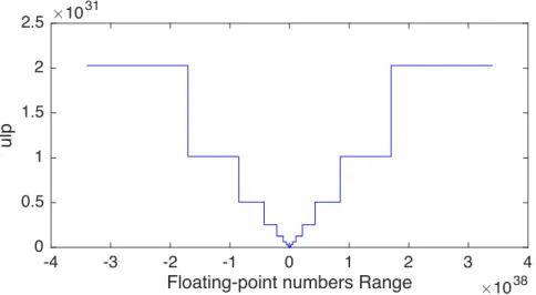
However, the introduced error can be reduced by clipping to the maximal (or minimal) repre-sentable value on overflow. This overflow mode is known as saturation.
2.4 Floating-point vs. Fixed-point
In this section, we compare floating-point and fixed-point representations based on different criteria, including range, precision, implementation cost and ease of use.
Range and Precision
The precision of a fixed-point representation <W, _, F > is determined by the scaling factor or the unit-in-last-position (ulp). It is a constant given by:
ulp = 2−F (2.10)
In a IEEE floating-point representation, the mantissa magnitude can represent a set of 2M
different floating-point numbers in the range [2exp, 2exp+1− 2exp−M], for a given exponent value
exp ∈ [−(2E−1− 2), 2E−1− 1] (in normalized mode). The unit-in-last-position (or precision) is
variable depending on the exponent value:
ulp = 2exp−M (2.11)
So all the numbers with same exponent have the same precision but numbers with higher expo-nent values are represented with lower precision as depicted in fig. 2.3. The range of representable floating-point positive numbers (normalized) is:
range = [2−(2E−1−2), 22E−1− 22E−1−1−M] (2.12)
Therefore, floating-point representation has the advantage to cover a much wider dynamic range but with adaptive precision, whereas fixed-point representation has a constant precision but covers a much narrower dynamic range.
Implementation
Hardware implementation of floating-point operators is expensive since it has to handle operands alignment, normalization, rounding and check for exceptions. This is mainly due to the fact that
Floating-point vs. Fixed-point 17
-4 -3 -2 -1 0 1 2 3 4
Floating-point numbers Range #1038 0 0.5 1 1.5 2 2.5 ulp #1031
Figure 2.3 – IEEE single-precision floating-point numbers precision vs. range.
the alignment requires a right shifter and the normalization requires a left/right shifter for up to M positions. Implementing these shifters is a trade-off between execution speed and cost. For example shift registers are cheap to implement but require a variable number of cycles depending on the shifting amount. Barrel shifters on the other hand can perform any shift in constant time but are expensive. Generally multi-level barrel shifters are used.
On the other hand, since fixed-point essentially uses integer arithmetic, no special hardware implementation is required to support it.
For this reason, many embedded processors do not provide support for floating-point arith-metic, for the sake of reducing cost and/or power consumption; they only provide integer compu-tation data-path. In order to perform real number compucompu-tations on such processors, two options are possible: either emulating floating-point, or implementing fixed-point arithmetic using the integer data-path.
Floating-point arithmetic emulation has a great impact on performance since a single floating-point operation often requires tens of integer arithmetic, shift and branch operations to perform alignment, normalization and rounding as mentioned earlier. Also representing floating-point data requires either more memory, in case mantissas and exponents are stored separately, or extra computations to encode/decode them if they are stored on the same word. This overhead can be even greater depending on the accuracy of the emulation and its compatibility with IEEE 754; a full compliant simulation requires checking and handling of exceptions.
On the other hand, fixed-point arithmetic can be emulated much faster when limited to use the integer data types natively supported by the target. In this case most fixed-point operations can be computed directly using the corresponding integer operator with additional shift operations when scalings are needed (assuming truncation is used as quantization, and no saturation). However, since this method is limited to the precision of the native data-types, quantization should be applied to keep intermediate operation results fit. This procedure is tedious, error
prone and hard to debug since the programmer must keep track of the (implicit) fixed-point formats, for every variable and intermediate operation result, and perform necessary scalings accordingly.
Alternatively, using full-fledged fixed-point libraries, such as Systemc, can seamlessly emulate any fixed-point format with precisions higher than the native data types and can emulate oper-ations with no precision loss. These libraries also support various quantization and saturation modes. But this is at the cost of much slower simulation speeds, by a factor of 20 to 400 as reported by Keding et al [50].
Therefore the only viable option when seeking tight performance and power consumption goals is to use native data types to represent fixed-point numbers and perform quantizations to keep data fit. To enhance the performance and precision of this approach, some specialized processors provide fixed-point specific enhancements such as:
— Pre-scaling of the input operands and/or post-scaling of the result. — Extended precision operators and registers.
— Hardware support for saturation and rounding.
Programmability
Most programming languages, like C/C++, provide native seamless support for standard floating-point data-types and operations but not for fixed-point; this is one of the reasons why most applications are developed using floating-point.
Floating-point is simpler to use, since the hardware does all the hard work providing an intuitive and straightforward interface. However, it can be very tricky in some cases. Floating-point immediate numbers are generally expressed in base 10 for the sake of simplicity. More often than not, these numbers cannot be exactly represented by the floating-point system being used (generally base 2), causing unintuitive behavior. For instance, comparing the result of operation 0.1 × 10 against 1 gives an unexpected result; both numbers are not equal as it might look like. Indeed, 0.1 is exactly representable in base 10 but not in base 2. In fact, C standard does not specify what base is used to represent floating-point data types, but in general it is base 2.
Conclusion
The characteristics of floating-point and fixed-point representations are summarized in ta-ble 2.2. Due to the high implementation cost of floating-point, fixed-point representation is often preferred in the context of ultra low power embedded applications. However, the devel-opment time is higher. Thus, automated floating-point to fixed-point conversion methodologies are required to cut down the time-to-market.
Floating-point to Fixed-point Conversion Methodologies 19
Representation Range Precision Cost Programmability Development Time Floating-point very wide variable high easy low
Fixed-point limited constant low difficult high Table 2.2 – Floating-point vs. Fixed-point.
2.5 Floating-point to Fixed-point Conversion Methodologies
As discussed earlier, floating-point is not suitable when targeting low power embedded proces-sors, and fixed-point is preferably used instead. Therefore, when applications are designed using floating-point, a floating-point to fixed-point conversion is required.
This conversion aims at attributing a fixed-point format to each floating-point data, and at replacing floating-point operations with fixed-point operations along with proper handling of scalings. This conversion may introduce computation errors due the overflows and/or quanti-zations. The conversion process must be aware of these errors and be able to estimate their effects in order to make sure that the computation accuracy remains within an "acceptable" limit specified by the developer, according to the application tolerance.
Overflows generally induce large errors. However, they can be prevented by evaluating the dy-namic value range of each variable and intermediate result and deducing, for each, the minimum IWLrequired to represent its value range. In this way overflows are mostly avoided. Alterna-tively, overflows can be allowed for cases with low occurrence probability to allow the use of smaller word-lengths. In this case saturation can be used to clip any overflow to the maximal (or minimal) value. In this case the induced errors should be analyzed since they may have a great impact on the computation accuracy.
In contrast, quantization errors are relatively small, but they can get amplified when prop-agated in the computation system and may result in a significant error at the system output. Therefore, it is very important to evaluate their effect on the computation accuracy and to make sure the latter stays within the specified limit.
Floating-point to fixed-point conversion generally involves three steps:
1. IWL determination of each variable and operation intermediate result in the system. 2. Word-length determination, to complement IWL determination in order to fully specify
the fixed-point formats. This generally makes the subject of an optimization, called Word Length Optimization (WLO).
3. Fixed-point code generation.
In the following, we discuss each of these steps.
2.5.1 Integer Word Length Determination
TheIWLof a variable is determined based on its dynamic value range. The aim is to specify the binary point position in the fixed-point formats in such a way to avoid overflows. The dynamic
range can be obtained either using simulation-based methods [64] or analytical methods. Simulation-based Methods
The floating-point code is instrumented to collect statistics on floating-point variables and operation results using simulations with representative input samples. The collected statistics are used to determine the dynamic ranges of the corresponding floating-point variables, which is then used to determine their IWL.
Simulation-based methods have the advantage to find tight ranges and therefore do not allocate unnecessary bits for the integer part. However, they do not guarantee the absence of overflows since the measured range depends on the tested input samples. thus, a large and representa-tive input samples must be used to obtain accurate enough estimations of the dynamic range. Regardless, overflows may still occur and in this case saturation can be used to limit overflow errors.
Analytical Methods
Alternatively, analytical methods can be used to derive the dynamic range of each variable and intermediate result, in a given system. Range propagation can be achieved using interval arithmetic or affine arithmetic for instance. In this case the input ranges are propagated through operations by a applying a correspondent propagation rule.
For example, using interval arithmetic we can deduce the range of variable y, at the output of the system depicted in fig. 2.4, given the range of inputs a, b and c. Let a ∈ [am, aM], b ∈ [bm, bM]
and c ∈ [cm, cM]. The intermediate result of the multiplication is then t ∈ [tm, tM], with:
tm = min(am× bm, aM × bM, am× bM, aM × bm) (2.13) tM = max(am× bm, aM × bM, am× bM, aM × bm) (2.14) Finally, y ∈ [tm+ cm, tM + cM]. * + a b c y
Figure 2.4 – Range propagation example.
Floating-point to Fixed-point Conversion Methodologies 21
a certain range that ensures the absence of overflows. However, the obtained ranges may be over-estimated resulting in unnecessary bits being allocated for the integer parts.
2.5.2 Word Length Optimization
The aim of this step is to select the word-length of each variable and operation in the system. TheFWLsare implicitly specified during this step following eq. (2.6), which directly affects the computation accuracy and performance. The word-length exploration space is generally specified depending on the target architecture. In the context ofHigh-Level Synthesis (HLS)[65] targeting FPGA for instance, a wide range of custom word-lengths can be considered. However, when targeting an off-the-shelf processor, word-lengths are generally restricted to the ones natively supported (e.g. 8, 16 or 32 bits) by the processor. In order to explore this solution space for each variable/operation, aWLOalgorithm [140, 85, 91] is generally used. It aims at selecting the best performance solution while maintaining accuracy within an "acceptable" limit. Therefore, this requires methodologies to evaluate the accuracy and the cost of a given fixed-point solution. Cost Estimation
When targeting embedded processors, the goal is generally to optimize the execution time (although energy consumption could be also considered). Execution time can be estimated by running the application and collecting timing measurements. To do so, the fixed-point code implementing the solution to be tested should be generated, compiled and run on the target processor with representative input data samples. This has the advantage to give a precise estimation of the execution time. However, this method greatly increases theWLOtime, since this needs to be done for each tested solution.
Alternatively, an estimation of the execution time can be obtained using static analysis or heuristic based on a cost model of the target architecture. Typically, a relative cost is associated to each operation type and size. In general, these methods do not lead to an accurate estimation of the execution time. However, it is often sufficient for comparing the cost between two different solutions.
Accuracy Evaluation
Accuracy evaluation aims at quantifying or measuring the accuracy of a given fixed-point solution. Many metrics can be used for this matter, such as Bit Error Rate (BER), generally used in communication applications, orSignal-to-Quantization-Noise Ratio (SQNR) often used in image/signal processing applications.
Simulation-based methods [128, 51, 65, 113] can be used for accuracy evaluation. They mainly consist of simulating the fixed-point system, with representative input samples, and comparing it against a baseline floating-point specification. The results are compared to find errors and compute the accuracy value. Such methods suffer from scalability issues, since the simulation time may be very high, specially in the context of design space exploration in which each tested
fixed-point solution should be simulated with enough input samples to evaluate its accuracy. This results in impractically long optimization times. On the other hand however, these methods have the advantage to be simple and applicable with no restrictions on the underlying computation system.
In order to cut-down the accuracy evaluation time, analytical methods [89, 87, 81, 83, 22, 109], aim at computing a closed-form generic expression, representing the fixed-point system accuracy, as a function of the number of bits assigned to different variables and operations in the system. Once this expression is generated, it can then be used to quickly evaluate the accuracy of any fixed-point solution for the system, by simply plugging-in the correspondent values of number of bits, making it more suitable for design space exploration. However, analytical methods are restricted to some particular systems, mainly Linear Time-Invariant (LTI) and non-recursive non-LTI systems.
For anLTIsystem, Menard and Sentieys [89] proposed a method to automatically compute the quantization noise power expression based on a computation of the transfer function of the system, represented by itsSignal Flow Graph (SFG). This is then used to determine theSQNR. Menard et al [87] later extended this method to cover non-LTI non-recursive systems using only one floating-point simulation to determine statistical parameters of noise sources and signal. These techniques evaluate the first moments (mean and variance) of the quantization noise sources and propagate it in the system to the output. To do so, the system is represented by its SFG, which can be constructed from the corresponding C code, but this requires flattening of all the control structures. For large systems, this make the computation of the analytical accuracy evaluation expression slow.
To solve this problem, Deest et al proposed an alternative, more scalable, representation [30] of the system based on the polyhedral model.
Shi and Brodersen proposed an alternative method [121] using a model of the quantization noise based on perturbation theory. This method uses simulations to compute the value of some parameters needed to obtain the analytical expression of the output noise power.
Alternative methods [81, 137] use affine arithmetic to represent the quantization noise in order to compute an analytical expression of the accuracy.
2.5.3 Fixed-point Code Generation
As discussed earlier, fixed-point can be simulated using C++ libraries such as Systemc and Algorithmic C Datatypes [1]. This solution has the advantage to seamlessly represent arbitrary-precision fixed-point formats and supports different overflow and quantization modes. However, it introduces a significant performance overhead as shown by Keding et al [50].
As mentioned earlier in section 2.4, the best performance option, when targeting embedded processor, is to limit fixed-point word-lengths to the natively supported ones. In this case, the fixed-point code can be generated using only native integer data-types to represent fixed-point


![Figure 3.6 – Example illustrating the difference between loop vectorization and SLP. [min : max]](https://thumb-eu.123doks.com/thumbv2/123doknet/14590410.730061/67.892.96.707.108.655/figure-example-illustrating-difference-loop-vectorization-slp-min.webp)