Mining (maximal) span-cores from temporal networks

HAL Id: hal-01863956

https://hal.archives-ouvertes.fr/hal-01863956

Submitted on 29 Aug 2018

HAL is a multi-disciplinary open access

archive for the deposit and dissemination of

sci-entific research documents, whether they are

pub-lished or not. The documents may come from

teaching and research institutions in France or

abroad, or from public or private research centers.

L’archive ouverte pluridisciplinaire HAL, est

destinée au dépôt et à la diffusion de documents

scientifiques de niveau recherche, publiés ou non,

émanant des établissements d’enseignement et de

recherche français ou étrangers, des laboratoires

publics ou privés.

Mining (maximal) span-cores from temporal networks

Edoardo Galimberti, Alain Barrat, Francesco Bonchi, Ciro Cattuto, Francesco

Gullo

To cite this version:

Edoardo Galimberti, Alain Barrat, Francesco Bonchi, Ciro Cattuto, Francesco Gullo.

Mining

(maximal) span-cores from temporal networks. CIKM2018, Oct 2018, Torino, Italy. pp.107-116,

�10.1145/3269206.3271767�. �hal-01863956�

Mining (maximal) span-cores from temporal networks

Edoardo Galimberti

University of Turin, Italy

edoardo.galimberti@isi.it

Alain Barrat

Aix Marseille Univ, CNRS, CPT, France

ISI Foundation, Italy

alain.barrat@cpt.univ- mrs.fr

Francesco Bonchi

Eurecat, Barcelona, Spain

francesco.bonchi@isi.it

Ciro Cattuto

ciro.cattuto@isi.it

Francesco Gullo

gullof@acm.org

ABSTRACT

When analyzing temporal networks, a fundamental task is the identification of dense structures (i.e., groups of vertices that exhibit

a large number of links), together with their temporal span (i.e., the period of time for which the high density holds). We tackle this

task by introducing a notion of temporal core decomposition where each core is associated with its span: we call such coresspan-cores.

As the total number of time intervals is quadratic in the size of the temporal domainT under analysis, the total number of span-cores is quadratic in|T | as well. Our first contribution is an algorithm that, by exploiting containment properties among span-cores, com-putes all the span-cores efficiently. Then, we focus on the problem

of finding only themaximal span-cores, i.e., span-cores that are not dominated by any other span-core by both the coreness property

and the span. We devise a very efficient algorithm that exploits the-oretical findings on the maximality condition to directly compute the maximal ones without computing all span-cores.

Experimentation on several real-world temporal networks con-firms the efficiency and scalability of our methods. Applications

on temporal networks, gathered by a proximity-sensing infrastruc-ture recording face-to-face interactions in schools, highlight the

relevance of the notion of (maximal) span-core in analyzing social dynamics and detecting/correcting anomalies in the data.

1

INTRODUCTION

A temporal network is a representation of entities (vertices), their

relations (links), and how these relations are established/broken along time. Extracting dense structures (i.e., groups of vertices ex-hibiting a large number of links among each other), together with

their temporal span (i.e., the period of time for which the high density is observed) is a key mining primitive. This type of

pat-terns enables fine-grain analysis of the network dynamics and can be a building block towards more complex tasks (such as finding

temporally recurring subgraphs or anomalously dense ones) and applications. For instance, they can help in studying the contact

networks among individuals to quantify the transmission oppor-tunities of respiratory infections, modeling situations where the

Permission to make digital or hard copies of all or part of this work for personal or classroom use is granted without fee provided that copies are not made or distributed for profit or commercial advantage and that copies bear this notice and the full citation on the first page. Copyrights for components of this work owned by others than the author(s) must be honored. Abstracting with credit is permitted. To copy otherwise, or republish, to post on servers or to redistribute to lists, requires prior specific permission and /or a fee. Request permissions from permissions@acm.org.

CIKM ’18, October 22–26, 2018, Torino, Italy

© 2018 Copyright held by the owner/author(s). Publication rights licensed to ACM. ACM ISBN 978-1-4503-6014-2/18/10. . . $15.00

https://doi.org/10.1145/3269206.3271767

risk of transmission is higher, with the goal of designing

mitiga-tion strategies [20]. Anomalously dense temporal patterns among entities in a co-occurrence graph (e.g., extracted from the

Twit-ter stream) have also been used to identify, in real-time, events and buzzing stories [2, 7]. In scientific collaboration and citation

networks these patterns can help understand the dynamics of col-laboration in successful professional teams, study the evolution of scientific topics, and detect emerging technologies [15].

In this paper we adopt as measure of density of a pattern the minimum degree holding among the vertices in the subgraph during

the pattern’s span. The problem of extractingall these patterns is tackled by introducing a notion oftemporal core decomposition

in which each core is associated with itsspan, i.e., an interval of contiguous timestamps, for which the coreness property holds.

To the best of our knowledge, this type of core, which we call

span-core, has never been studied so far.

Challenges and contributions. As the total number of time inter-vals is quadratic in the size of the temporal domainT under analysis, also the total number of span-cores is, in the worst case, quadratic in T . Nevertheless, exploiting nice containment properties we devise an efficient algorithm for computing all thespan-cores. Then, we shift our attention to the problem of finding only themaximal span-cores, i.e., span-cores that are not dominated by any other span-core

by both the coreness property and the span. A straightforward way of approaching the maximal-span-core-mining problem is to filter

out non-maximal span-cores during the execution of an algorithm for computing the whole span-core decomposition. However, as

the maximal ones are usually much less than the overall span-cores, it would be desirable to have a method that effectively exploits the maximality property and extracts maximal span-cores directly,

without computing a complete decomposition. The design of an algorithm of this kind is an interesting challenge, as it contrasts

the intrinsic conceptual properties of core decomposition, based on which a core of orderk can be efficiently computed from the core of orderk −1, of which it is a subset. For this reason, at first glance, the computation of the core of the highest order would seem

as hard as computing the overall core decomposition. Instead, in this work we derive a number of theoretical properties about the relationship among span-cores of different temporal intervals and,

based on these findings, we show how such a challenging goal may be achieved.

The contributions of this paper can be summarized as follows:

• We introduce the notion of span-core decomposition and maxi-mal span-core in temporal networks. We characterize structure

and size of the search space, and prove important containment properties (Section 3).

• We devise an algorithm for computing all span-cores that exploits the aforementioned containment properties and is orders of magnitude faster than a naïve method based on

traditional core decomposition (Section 4).

• We study the problem of finding only the maximal span-cores. We derive a number of theoretical findings about the relation-ship among maximal span-cores and exploit them to devise an

algorithm that is more efficient than computing all span-cores and discarding the non-maximal ones (Section 5).

• We provide a comprehensive experimentation on several real-world temporal networks, with millions of vertices, tens of millions of edges, and hundreds of timestamps, which attests

efficiency and scalability of our methods (Section 6).

• We present applications on face-to-face interaction networks, that illustrate the relevance of the notion of (maximal) span-core in real-life analyses (Section 7).

The next section overviews the related literature, while Section 8

discusses future work and concludes the paper.

2

BACKGROUND AND RELATED WORK

Core decomposition. In standard graphs, among the many def-initions of dense structures,core decomposition plays a central role as it can be computed in linear time [5, 31], and can

speed-up/approximate dense-subgraph extraction according to various other definitions. For instance, core decomposition allows for find-ing cliques more efficiently [14], it can be used to approximate the

densest-subgraph problem [27], and betweenness centrality [22]. Given a simple graphG = (V , E), let d(S,u) denote the degree of vertexu ∈ V in the subgraph induced by vertex set S ⊆ V , i.e., d (S,u) = |{v ∈ S | (u,v) ∈ E}|.

Definition 1 (Core Decomposition). Thek-core (or core of orderk) of G is a maximal set of vertices C_k ⊆V such that ∀u ∈ Ck :d (C_k,u) ≥ k. The set of all k-cores V = C0⊇C1 ⊇ · · · ⊇Ck∗

(k∗= arg max_kC_{k, ∅) is the core decomposition of G.}

Core decomposition has been established as an important tool to analyze and visualize complex networks [1, 4] in several

do-mains, e.g., bioinformatics [3, 42], software engineering [43], and social networks [18, 26]. It has been studied under various settings,

such as distributed [33], streaming/maintenance [29, 36], and disk-based [10], and for various types of graph, such as uncertain [8],

directed [21], and weighted graphs [17].

Core decomposition inmultilayer networks has been studied in [16]. As any subset of layers is allowed in this setting, the total

number of cores is intrinsically exponential. Although temporal networks can be seen as a special case of multilayer networks

(where each timestamp is interpreted as a layer), the sequentiality of time represents an important structural constraint: in this paper

we are interested in cores that span a temporal interval, and not simply any subset of (potentially non-contiguous) timestamps. As a

consequence, the search space and the number of cores are no longer exponential as in the multilayer case. A type of core decomposition for temporal networks has been proposed by Wuet al. [41], who

define the(k, h)-core as the largest subgraph in which every vertex has at leastk neighbors and at least h temporal connections with each of them. Therefore, even in the Wuet al.’s definition the

sequentiality of connections is not taken into account and

non-contiguous timestamps can support the same core. Our temporal cores have instead a clear temporal collocation and continuous

spans, thus the Wuet al.’s definition cannot be reduced to ours (or vice versa). As we will see in Section 7, such a temporal collocation

is important in applications.

Patterns in temporal networks. Semertzidis et al. [37] intro-duce the problem of identifying a set of vertices that are densely connected in all or at leastk timestamps of a temporal network. Similarly, Jethava and Beerenwinkel [25] formulate the densest-common-subgraph problem on an input that can be interpreted

as a special type of temporal network, i.e., a set of graphs sharing the same vertex set. The notion of∆-clique has been proposed in [23, 40], as a set of vertices in which each pair is in contact at

least every∆ timestamps. Complementary approaches study the problem of discovering dense temporal subgraphs whose edges

occur in short time intervals considering the exact timestamp of the occurrences [34], and the problem of maintaining the densest

subgraph in the dynamic graph model [13]. A slightly different, but still related body of literature focuses on frequent evolution patterns in temporal attributed graphs [6, 12, 24], link-formation

rules in temporal networks [9, 28], and the discovery of dynamic relationships and events [11] or of correlated activity patterns [19].

3

PROBLEM DEFINITION

We are given atemporal graphG = (V ,T,τ ), where V is a set of vertices,T = [0, 1, . . . , tmax]⊆ N is a discrete time domain, and τ : V ×V ×T → {0, 1} is a function defining for each pair of vertices u,v ∈ V and each timestamp t ∈ T whether edge (u,v) exists in t. We denote E = {(u,v, t) | τ (u,v, t) = 1} the set of all temporal edges. Given a timestampt ∈ T , E_t = {(u,v) | τ (u,v, t) = 1} is the set of edges existing at timet. A temporal interval ∆ = [t_s, t_e] is contained into another temporal interval∆′= [t_s′, t_e′], denoted ∆ ⊑ ∆′

, ift_s′≤ts andt_e′≥te. Given an interval∆ ⊑ T , we denote E∆ = Tt ∈∆Etthe edges existing inall timestamps of∆. Given a subsetS ⊆ V of vertices, let E_∆[S] = {(u,v) ∈ E_∆ |u ∈ S,v ∈ S} andG_∆[S] = (S, E_∆[S]). Finally, the temporal degree of a vertex u withinG_∆[S] is denoted d_∆(S,u) = |{v ∈ S | (u,v) ∈ E_∆[S]}|.

Definition 2 ((k, ∆)-core). The (k, ∆)-core of a temporal graph G = (V ,T,τ ) is (when it exists) a maximal and non-empty set of vertices∅ , C_k,∆ ⊆V , such that ∀u ∈ C_k,∆ :d_∆(C_k,∆,u) ≥ k, where∆ ⊑ T is a temporal interval and k ∈ N+.

A(k, ∆)-core is a set of vertices implicitly defining a cohesive subgraph (wherek represents the cohesiveness constraint), together with itstemporal span, i.e., the interval∆ for which the subgraph satisfies the cohesiveness constraint. In the remainder of the paper we refer to this type of temporal pattern asspan-core.

The first problem we tackle in this work is to compute the span-core decomposition of a temporal graphG, i.e., all span-cores of G.

Problem 1 (Span-core decomposition). Given a temporal graph G, find the set of all (k, ∆)-cores of G.

Unlike standard cores of simple graphs, span-cores are not all

nested into each other, due to their spans. However, they still exhibit containment properties. Indeed, it can be observed that a(k, ∆)-core is contained into any other(k′, ∆′)-core with less restrictive

degree and span conditions, i.e.,k′≤k, and ∆′⊑∆. This property is depicted in Figure 1, and formally stated in the next proposition.

Proposition 1 (Span-core containment). For any two span-coresC_k,∆,C_k′_,∆′of a temporal graphG it holds that

k′_{≤k ∧ ∆}′_{⊑∆ ⇒ C}

k,∆ ⊆C_k′_,∆′.

Proof. The result can be proved by separating the two condi-tions in the hypothesis, i.e., by separately showing that (i) k′≤k ⇒ Ck,∆ ⊆C_k′_,∆, and (ii) ∆′⊑∆ ⇒ C_k,∆⊆C_k,∆′. The first argument holds as, keeping the span∆ fixed, the maximal set of vertices C for whichd_∆(C,u) ≥ k is clearly contained in the maximal set of verticesC′for whichd_∆(C′,u) ≥ k′, ifk′≤k. As far as the second argument, it can be noted that∆′⊑∆ ⇒ E_∆⊆E_∆′, which implies that∀u ∈ C_k,∆:d_∆(C_k,∆,u) ≤ d_∆′(C_k,∆,u). Therefore, all vertices

withinC_k,∆satisfy the condition to be part ofC_k,∆′too. □ Observation 1. For a fixed temporal interval∆ ⊑ T , finding all span-cores that have∆ as their span is equivalent to computing the classic core decomposition [5] of the simple graphG_∆= (V , E_∆).

As the total number of temporal intervals that are contained into the whole time domainT is |T |(|T | +1)/2, the total number of span-cores isO(|T |2×k_max), where k_maxis the largest value ofk for which a (k, ∆)-core exists. The number of span-cores is thus quadratic in|T |, which may be too large an output for human inspection. In this regard, it may be useful to focus only on the

most relevant cores, i.e., themaximal ones, as defined next.

Definition 3 (Maximal Span-core). A span-coreC_k,∆of a tem-poral graphG is said maximal if there does not exist any other span-coreC_k′_,∆′ofG such that k ≤ k′and∆ ⊑ ∆′.

Hence, a span-core is recognized as maximal if it is not

domi-nated by another span-core both on the orderk and the span ∆. Differently from theinnermost core (i.e., the core of the highest

order) in the classic core decomposition, which is unique, in our temporal setting the number of maximal span-cores isO(|T |2), as, in the worst case, there may be one maximal span-core for every

temporal interval. However, as observed experimentally, maximal span-cores are always much less than the overall span-cores: the

difference is usually one order of magnitude or more. The second problem we tackle in this work is to compute the maximal

span-cores of a temporal graph.

Problem 2 (Maximal Span-core Mining). Given a temporal

graphG, find the set of all maximal (k, ∆)-cores of G.

Clearly, one could solve Problem 2 by solving Problem 1 and fil-tering out all the non-maximal span-cores. However, an interesting

yet challenging question (Section 5) is whether one can exploit the maximality condition to develop faster algorithms that can directly

extract the maximal ones, without computing all the span-cores.

4

COMPUTING ALL SPAN-CORES

In this section we devise algorithms for computing a complete span-core decomposition of a temporal graph (Problem 1). A naïve approach. As stated in Observation 1, for a fixed temporal interval∆ ⊑ T , mining all span-cores C_k,∆is equivalent to comput-ing the classic core decomposition of the graphG_∆= (V , E_∆). A

2,[1,2] 3,[1,2] 1,[1,2] 2,[1,1] 3,[1,1] 1,[1,1] 2,[0,1] 3,[0,1] 1,[0,1] 2,[0,0] 3,[0,0] 1,[0,0] 2,[2,2] 3,[2,2] 1,[2,2] 2,[2,3] 3,[2,3] 1,[2,3] 2,[3,3] 3,[3,3] 1,[3,3] 1,[0,3] 2,[1,3] 3,[1,3] 1,[1,3] 2,[0,2] 3,[0,2] 1,[0,2]

Figure 1: Search space: for a temporal span∆ = [ts, te], the (k, ∆)-core is depicted as a node labeled “k, [ts, te]”. An arrow C1→C2denotesC1⊇C2(distinction between solid and

dot-ted arrows is for visualization sake only).

naïve strategy is thus to run a core-decomposition subroutine [5]

on graphG_∆for each temporal interval∆ ⊑ T . Such a method has time complexityO(P_∆⊑T(|∆| × |E|)), i.e., O(|T |2× |E|).

A more efficient algorithm. Looking at Figure 1 one can observe that the naïve algorithm only exploits one dimension of the

con-tainment property: it starts from each point on the top level, i.e., from cores of order 1, and goes down vertically with the classic

core decomposition. Based on Proposition 1, it is possible to de-sign a more efficient algorithm that exploits also the “horizontal

containment” relationships.

Example 1. Consider coreC_1,[0,2] in Figure 1: by Proposition 1 it holds that it is a subset of bothC_1,[0,1]andC_1,[1,2]. Therefore, to computeC_1,[0,2], instead of starting from the wholeV , one can start fromC_1,[0,1]∩C_1,[1,2]. Starting from a much smaller set of vertices can provide a substantial speed-up to the whole computation.

This observation, although simple, produces a speed-up of orders of magnitude as we will empirically show in Section 6. The next

straightforward corollary of Proposition 1 states that, not only C1,[0,2] ⊆C1,[0,1]∩C1,[1,2], but this is the best one can get, meaning

that intersecting these two span-cores is equivalent to intersecting

all span-cores structurally containingC_1,[0,2].

Corollary 1. Given a temporal graphG = (V ,T,τ ), and a tem-poral interval∆ = [t_s, t_e]⊑T , let ∆₊ = [min{t_s + 1, t_e}, t_e]and ∆−= [ts, max{te− 1, ts}]. It holds that

C1,∆ ⊆ (C1,∆₊∩C1,∆−) =

\

∆′_⊑∆

C1,∆′.

Example 2. Consider againC_1,[0,2] in Figure 1: Proposition 1 states that it is a subset ofC

1,[0,0],C1,[0,1],C1,[1,1],C1,[1,2],C1,[2,2].

Corollary 1 suggests that there is no need to intersect them all, but onlyC_1,[0,1] andC_1,[1,2]: in fact,C_1,[0,1] ⊆C_1,[0,0]∩C_1,[1,1]and C1,[1,2] ⊆C1,[1,1]∩C1,[2,2].

The main idea behind our efficientSpan-cores algorithm (whose pseudocode is given as Algorithm 1) is to generate temporal

in-tervals of increasing size (starting from size one) and, for each∆ of width larger than one, to start the core decomposition from (C1,∆₊∩C1,∆−), i.e., the smallest intersection of cores containing

Algorithm 1: Span-cores

Input: A temporal graphG = (V, T, τ ). Output: The set C of all span-cores ofG.

1 C ← ∅; Q ← ∅; A ← ∅

2 forallt ∈ T do

3 enqueue [t, t ] to Q; A[t, t ] ← V

4 whileQ , ∅ do

5 dequeue∆ = [t_s, t_e] fromQ

6 E∆[A[∆]] ← {(u, v ) ∈ E_{∆ |}u ∈ A[∆], v ∈ A[∆]}

7 if |E∆[A[∆]]| > 0 then

8 C∆←core-decomposition( A[∆], E∆[A[∆]])

9 C ← C ∪ C∆

10 ∆1= [max{ts− 1, 0}, te]; ∆2= [ts, min{te+ 1, tmax}]

11 forall∆′∈ {∆1, ∆2} |∆′, ∆ do

12 if A[∆′]_{, null then}

13 A[∆′]← A[∆′]∩C1,∆

14 enqueue∆′toQ

15 else

16 A[∆′]←C1,∆

C1,∆(Corollary 1). The intervals to be processed are added to queue

Q, which is initialized with the intervals of size one (Lines 2–3): these are the only intervals for which no other interval can be used

to reduce the set of vertices from which start the core decomposi-tion, thus it has to be initialized with the whole vertex setV . The algorithm utilizes a mapA that, given an interval∆, returns the set of vertices to be used as a starting set of the core decomposi-tion on∆. The algorithm processes all intervals stored in Q, until Q has become empty (Lines 4–16). For every temporal interval ∆ extracted fromQ, the starting set of vertices is retrieved from A[∆] and the corresponding set of edges is identified (Line 6). Unless this is empty, the classic core-decomposition algorithm [5] is invoked

over(A[∆], E_∆[A[∆]]) (Line 8) and its output (a set of span-cores of span∆) is added to the ultimate output set C (Line 9).

Afterwards, the two intervals, denoted∆₁and∆₂, for whichC_1,∆ can be used to obtain the smallest intersections of cores containing them (Corollary 1) are computed at Line 10. For∆1(and analogously

∆2), we check whetherA[∆1] has already been initialized (Line 12):

this would mean that previously the other “father” (i.e., smallest

containing core) ofC1,∆1has been computed, thus we can intersect

C1,∆withA[∆1] and enqueue∆1to be processed (Lines 13–14).

Instead, ifA[∆₁] was not yet initialized, we initialize it withC_1,∆ (Line 16): in this case∆1is not enqueued because it still misses one

father to be intersected before being ready for core decomposition.

This procedural update ofQ ensures that both fathers of every interval inQ exist and have been previously computed, thus no a-posteriori verification is needed.

Example 3. Consider again the search space in Figure 1.

Algo-rithm 1 first processes the intervals [0, 0], [1, 1], [2, 2], and [3, 3]. Then, it intersectsC_1,[0,0]andC_1,[1,1]to initializeC_1,[0,1], intersectsC_1,[1,1] andC

1,[2,2]to initializeC1,[1,2], and intersectsC1,[2,2]andC1,[3,3]

to initializeC_1,[2,3]. Then, it continues with the intervals of size 3: it intersectsC

1,[0,1]andC1,[1,2]to initializeC1,[0,2]and so on.

The next theorem formally shows soundness and completeness of ourSpan-cores algorithm.

Theorem 1. Algorithm 1 is sound and complete for Problem 1.

Proof. The algorithm generates and processes a subset of tem-poral intervalsX ⊆ {∆ | ∆ ⊑ T }. For every interval ∆ ⊆ X, it computesall span-coresC_∆ = {C1,∆,C2,∆, . . . ,Ck_∆,∆} defined

on ∆ by means of the core-decomposition subroutine on the graph(A[∆], E_∆[A[∆]]). The set of vertices A[∆] is equivalent to (C1,∆₊∩C1,∆−) because of Line 13 (Corollary 1) and the fact that ∆

is enqueued (Line 14) only when both fathers have been processed

and the intersection done. The correctness of doing the classic core decomposition is guaranteed by Observation 1.

As for completeness, it suffices to show that the intervals∆ < X that have not been processed by the algorithm do not yield any

span-core. The algorithm generates all temporal intervals size by size, starting from those of size one and then going to larger sizes. This is done by maintaining the queueQ. As said above, an interval ∆ is enqueued as soon as both C1,∆₊andC1,∆−have been processed.

Thus, an interval∆ is not in X only if either C_1,∆

+orC1,∆−does not

exist. In this caseC1,∆and all otherCk,∆do not exist as well. □

Discussion. Algorithm 1 exploits the “horizontal containment” relationships only at the first level of the search space. For a given ∆, once the restricted starting set of vertices has been defined for k = 1, the traditional core decomposition is started to produce all the span-cores of span∆. In other words, for k > 1 only the “vertical containment” is exploited. Consider the span-coreC_3,[1,2] in Figure 1: we know that it is a subset ofC_2,[1,2](“vertical” ) and of C3,[1,1]andC3,[2,2](“horizontal” ). One could consider intersecting

all these three span-cores before computingC_3,[1,2]. We tested this alternative approach, but concluded that the overhead of computing

intersections and data-structure maintenance was outweighing the benefit of starting from a smaller vertex set.

The worst-case time complexity of Algorithm 1 is equal to the

naïve approach, however in practice it is orders of magnitude faster, as shown in Section 6.

5

COMPUTING MAXIMAL SPAN-CORES

In this section we focus on Problem 2: computing themaximal

span-cores of a temporal graph.

A filtering approach. As anticipated above, a straightforward way of solving this problem consists in filtering the span-cores

computed during the execution of Algorithm 1, so as to ultimately output only the maximal ones. This can easily be accomplished by equipping Algorithm 1 with a data structureM that stores the span-core of the highest order for every temporal interval∆ ⊑ T that has been processed by the algorithm. Moreover, at the storage

of a span-coreC_k,∆inM, the span-cores previously stored in M for subintervals of the temporal interval∆ and with the same order k are removed from M. This removal operation, together with the order in which span-cores are processed, ensures thatM eventually contains only the maximal span-cores.

Efficient maximal-span-core finding. Our next goal is to design a more efficient algorithm that extracts maximal span-cores directly, without computing complete core decompositions, passing over

more peripheral ones, and without generating all temporal cores. This is a quite challenging design principle, as it contrasts the

a core of orderk is usually computed from the core of order k −1, thus making the computation of the core of the highest order as hard as computing the overall decomposition. Nevertheless, thanks

to theoretical properties that relate the maximal span-cores to each other, in the temporal context such a challenge can be achieved. In

the following we discuss such properties in detail, by starting from a result that has already been discussed above, but only informally. Consider the classic core decomposition in a standard

(non-temporal) graphG (Definition 1) and let C_k∗[G] denote the in-nermost core ofG, i.e., the non-empty k-core of G with the largest k. Lemma 1. Given a temporal graphG = (V ,T,τ ), let C_Mbe the set of all maximal span-cores ofG, and C_inner= {C_k∗[G_∆]|∆ ⊑ T } be the set of innermost cores of all graphsG_∆. It holds thatC_M ⊆C_inner. Proof. EveryC_k,∆ ∈ C_M is the innermost core of the non-temporal graphG_∆: else, there would exist another coreC_k′_{,∆, ∅}

withk′> k, implying that C_{k,∆< CM}. □ Lemma 1 states that each maximal span-core is an innermost core of aG_∆, for some temporal interval∆ ⊑ T . Hence, there can exist at most one maximal span-core for every∆ ⊑ T (while an interval∆ may not yield any maximal span-core). The key question to design an efficient maximal-span-core-mining algorithm thus

becomes how to extract innermost cores of the graphsG_∆more efficiently than by computing the full core decompositions of all G∆. The answer to this question comes from the result stated in the next two lemmas (with Lemma 2 being auxiliary to Lemma 3).

Lemma 2. Given a temporal graphG = (V ,T,τ ), and three tem-poral intervals ∆ = [t_s, t_e] ⊑ T , ∆′ = [t_s− 1, t_e] ⊑ T , and ∆′′ _{= [t}

s, te+1] ⊑ T . The innermost core Ck∗[G_∆]is a maximal span-core ofG if and only if k∗> max{k′, k′′} wherek′andk′′are the orders of the innermost cores ofG_∆′andG_∆′′, respectively.

Proof. The “⇒” part comes directly from the definition of maxi-mal span-core (Definition 3): ifk∗were not larger than max{k′, k′′}, thenC_k∗[G_∆] would be dominated by another span-core both on the order and on the span (as both∆′and∆′′are superintervals of ∆). For the “⇐” part, from Lemma 1 and Proposition 1 it follows that max{k′, k′′} is an upper bound on the maximum order of a span-core of a superinterval of∆. Therefore, k∗ > max{k′, k′′} implies that there cannot exist any other span-core that dominates Ck∗[G_∆] both on the order and on the span. □ Lemma 3. GivenG, ∆, ∆′,∆′′,k′, andk′′defined as in Lemma 2, let HV = {u ∈ V | d_∆(V ,u) > max{k′, k′′}}, and letC_k∗[G_∆[HV ]] be the innermost core ofG_∆[HV ]. If k∗> max{k′, k′′}, thenC_k∗[G_∆[HV ]] is a maximal span-core; otherwise, no maximal span-core exists for∆. Proof. Lemma 2 states that, to be recognized as a maximal span-core, the innermost core ofG_∆should have order larger than max{k′, k′′}. This means that, if the innermost core ofG_∆is a maxi-mal span-core, all verticesu <V cannot be part of it. Therefore, GH ∆ yields a maximal span-core only if the innermost core of subgraph G∆[HV ] has order k∗> max{k′, k′′}. □ Lemma 3 provides the basis of our efficient method for extracting maximal span-cores. Basically, it states that, to verify whether a

certain temporal interval∆ = [ts, te] yields a maximal span-core

Algorithm 2: Maximal-span-cores Input: A temporal graphG = (V, T, τ ).

Output: The set CMof all maximal span-cores ofG.

1 CM← ∅ 2 K′[t ] ← 0, ∀t ∈ T 3 forallts ∈ [0, 1, . . . , tmax]do 4 t∗← max {te ∈ [ts, tmax]_|E [_{ts ,te ]}, ∅ } 5 k′′← 0 6 forallte ∈ [t∗, t∗−1, . . . , ts]do 7 ∆ ← [ts, te] 8 lb ← max{K′[t_e], k′′} 9 V_{l b}← {u ∈ V | d∆(V , u) > lb } 10 E∆[V_{l b}]← {(u, v ) ∈ E_∆|u ∈ V_{l b}, v ∈ V_{l b}} 11 C ← innermost-core(V_{l b}, E∆[V l b]) 12 k∗← order ofC 13 ifk∗> lb then 14 CM←CM∪ {C } 15 k′′← max {k′′, k∗}; K′[t_e]_{← max { K}′[t_e], k′′_}

(and, if so, compute it), there is no need to consider the whole graphG_∆, rather it suffices to start from a smaller subgraph, which is given by all vertices whose temporal degree is larger than the maximum between the orders of the innermost cores of intervals ∆′_{= [t}

s−1, t_e] and∆′′= [ts, te+1]. This finding suggests a strategy that is opposite to the one used for computing the overall span-core decomposition: atop-down strategy that processes temporal

inter-vals starting from the larger ones. Indeed, in addition to exploiting the result in Lemma 3, this way of exploring the temporal-interval

space allows us to skip the computation of complete core decompo-sitions of the whole “singleton-interval” graphs{G

[t, t ]}t ∈T, which

may easily become a critical bottleneck, as they are the largest ones among the graphs induced by temporal intervals.

The Maximal-span-cores algorithm. Algorithm 2 iterates over all timestampst_s ∈T in increasing order (Line 3), and for each t_s it first finds all the maximal span-cores that have span starting in ts. This way of proceedingensures that a span-core that is recog-nized as maximal will not be later dominated by another span-core.

Indeed, an interval [ts, te] can never be contained in another inter-val [t_s′, t_e′] witht_s < t_s′. For a givent_s, all maximal span-cores are computed as follows. First, the maximum timestamp≥t_s such that the corresponding edge setE

[_{ts ,te ]}is not empty is identified ast ∗

(Line 4). Then, all intervals∆ = [ts, te] are considered one by one indecreasing order oft_e(Lines 6–7): this againguarantees that a span-core that is recognized as maximal will not be later dominated

by another span-core, as the intervals are processed from the largest to the smallest. At each iteration of the internal cycle, the algorithm

resorts to Lemma 3 and computes the lower boundlb on the order of the innermost core ofG_∆to be recognized as maximal, by taking the maximum betweenK′[te] andk′′(Line 8).K′is a map that maintains, for every timestampt ∈ [t_s, t∗], the order of the inner-most core of graphG_∆′, where∆′ = [ts− 1, t] (i.e., K′[t] stores what in Lemmas 2–3 is denoted ask′). Whereask′′stores the order of the innermost core ofG_∆′′, where∆′′= [t_s, t_e+ 1]. Afterwards, the sets of verticesV_lband of edgesE_∆[V_lb] that comply with this lower-bound constraint are built (Lines 9–10), and the innermost

core of the subgraph(V_lb, E_∆[V_lb]) is extracted (Lines 11–12). Ulti-mately, based again on Lemma 3, such a core is added to the output set of maximal span-cores only if its order is actually larger thanlb (Lines 13–14), and the values ofk′′andK′[te] are updated (Line 15). Specifically, note that the orderk∗of coreC may in principle be less thank′′, asC is extracted from a subgraph of G_∆. If this happens, it means that the actual order of the innermost core ofG_∆is equal tok′′. This motivates the update rules (and their order) reported in Line 15.

Theorem 2. Algorithm 2 is sound and complete for Problem 2.

Proof. The algorithm processes all temporal intervals∆ ⊑ T yielding a non-empty edge setE_∆, in an order such that no interval is processed before one of its superintervals: this guarantees that a

span-core recognized as maximal will not be dominated by another span-core found later on. For every∆ it extracts a core C that is used as a proxy of the innermost core of graphG_∆.C is added to the output setC_M only if Lemma 3 recognizes it as a maximal span-core, otherwise it is discarded. This proves the soundness of

the algorithm. Completeness follows from Lemma 1, which states that to extract all maximal span-cores it suffices to focus on the

innermost cores of graphs{G_∆ | ∆ ⊑ T }, and Lemma 3 again, which states the condition for a proxy coreC to be safely discarded

because it is a non-maximal span-core. □

Discussion. The worst-case time complexity of Algorithm 2 is the same as the algorithm for computing the overall span-core

decomposition, i.e.,O(|T |2× |E|). It is worth mentioning that it is not possible to do better than this, as the output itself is potentially

quadratic in|T |. However, as we will show in Section 6, the proposed algorithm is in practice much more efficient than computing the

overall span-core decomposition and filtering out the non-maximal cores as, in this case, we avoid the visit of portions of the

span-core search space and the computations are run over subgraphs of reduced dimensions.

To conclude, we discuss how the crucial operation of building the

subgraph(V_lb, E_∆[V_lb]) may be carried out efficiently in terms of both time and space. Consider a fixed timestampt_s ∈ [0, . . . , t_max]. The following reasoning holds for everyts. LetE−(te) = E

[_{ts ,te ]}\

E[_{ts ,te+1]}be the set of edges that are inE[_{ts ,te ]}but not inE[_{ts ,te+1]}, for

te∈ [ts, . . . , t∗− 1]. As a first general step, for eacht_s, we compute and storeall edge sets{E−(t_e)}_te∈[ts,t∗_−1]. These operations can be accomplished inO(|T | × |E|) overall time, because every E−(t_e) can be computed incrementally fromE

[_{ts ,te ]}asE −_(t

e) = {(u,v) ∈

E[_{ts ,te ]} |τ (u,v, te+1) = 0}. Moreover, for any timestamp te

, we

keep a mapD storing all vertices ofG

[_{ts ,te ]}organized by degree.

Specifically, the setD[k] contains all vertices having degree > k inG

[_{ts ,te ]}. Every vertex inD is thus replicated a number of times

equal to its degree. This way, the overall space taken byD is O(|E|), i.e., as much space asG. D is initialized as empty (when te = t∗) and repeatedly augmented ast_edecreases, by a linear scan of the variousE−(te). The overall filling of D (for all te) therefore takes O(|T |×|E|) time. Then, the desired V_lbcan be computed in constant time simply asV_lb= D[lb].

As for E_∆[V_lb], for any t_e, we first reconstruct E

[_{ts ,te ]} as

E[_{ts ,te +1]}∪E −_(t

e), having previously computed E[_{ts ,te +1]}

. Note that

storing allE−(t_e) takes O(|E|) space. That is why we store all

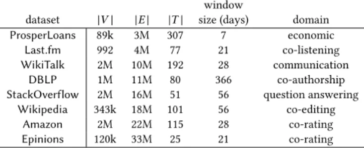
Table 1:Temporal graphs used in the experiments. window

dataset |V | |E | |T | size (days) domain

ProsperLoans 89k 3M 307 7 economic

Last.fm 992 4M 77 21 co-listening

WikiTalk 2M 10M 192 28 communication

DBLP 1M 11M 80 366 co-authorship

StackOverflow 2M 16M 51 56 question answering

Wikipedia 343k 18M 101 56 co-editing

Amazon 2M 22M 115 28 co-rating

Epinions 120k 33M 25 21 co-rating

E−_(t

e) and reconstruct E[_{ts ,te ]}

afterward (instead of storing the

latter, which would takeO(|T | × |E|) space). E_∆[V_lb] is ultimately derived by a linear scan ofE

[_{ts ,te ]}

, taking all edges inE

[_{ts ,te ]}

having

both endpoints inV_lb. This way, the step of buildingE_∆[V_lb] for allt_etakes againO(|T | × |E|) overall time.

6

EXPERIMENTS

In this section we present a performance comparison of our

algo-rithms, as well as a characterization of span-cores extracted. Datasets. We use eight real-world datasets recording timestamped interactions between entities.1For each dataset we select a window size to define a discrete time domain, composed of contiguous timestamps of the same duration, and build the corresponding

temporal graph. If multiple interactions occur between two entities during the same discrete timestamp, they are counted as one. The

characteristics of the resulting temporal graphs, along with the selected window sizes (in days), are reported in Table 1.

ProsperLoans represents the network of loans between the users of Prosper, a marketplace of loans between privates.Last.fm records the co-listening activity of the Last.fm streaming platform: an edge

exists between two users if they listened to songs of the same band within the same discrete timestamp.WikiTalk is the communica-tion network of the English Wikipedia.DBLP is the co-authorship network of the authors of scientific papers from the DBLP

com-puter science bibliography.StackOverflow includes the answer-to-question interactions on the stack exchange of the stackover-flow.com website.Wikipedia connects users of the Italian Wikipedia that co-edited a page during the same discrete timestamp. Finally, for bothAmazon and Epinions, vertices are users and edges rep-resent the rating of at least one common item within the same discrete timestamp.

Implementation. All methods are implemented in Python (v. 2.7.12) and compiled by Cython. The experiments run on a ma-chine equipped with Intel Xeon CP U at 2.1GHz and 64GB RAM. Reproducibility. Our code is available at goo.gl/4WmrPc.

6.1

Span-core decomposition

We compare the two methods to compute a complete decomposition

described in Section 4, i.e., the baselineNaïve-span-cores and the proposedSpan-cores, in terms of execution time, memory, and total number of vertices input to thecore-decomposition subroutine. We report these measures, together with the numbers of span-cores and maximal span-cores of each dataset, in Table 2.

1

All datasets are made available by the KONECT Project (http://konect.cc), except for StackOverflow which is part of the SNAP Repository (http://snap.stanford.edu).

Table 2:Evaluation of the proposed algorithms: number of output span-cores, time, memory, and number of processed vertices.

# output time memory # processed dataset method span-cores (s) (GB) vertices ProsperLoans Naïve-span-cores 4 273 101 2 55M Span-cores 46 2 27M Naïve-maximal-span-cores 293 48 2 27M Maximal-span-cores 8 2 980k Last.fm Naïve-span-cores 126 819 707 0.5 2M Span-cores 199 0.5 531k Naïve-maximal-span-cores 1 670 202 0.5 531k Maximal-span-cores 57 0.5 271k WikiTalk Naïve-span-cores 19 693 322 302 36 25B Span-cores 1 084 36 555M Naïve-maximal-span-cores 632 1 194 36 555M Maximal-span-cores 126 35 2M DBLP Naïve-span-cores 6 135 10 506 11 1B Span-cores 278 11 150M Naïve-maximal-span-cores 268 292 11 150M Maximal-span-cores 116 11 620k StackOverflow Naïve-span-cores 1 238 5 360 10 1B Span-cores 245 10 127M Naïve-maximal-span-cores 129 245 10 127M Maximal-span-cores 128 10 3M Wikipedia Naïve-span-cores 125 191 17 155 4 1B Span-cores 522 4 35M Naïve-maximal-span-cores 2 147 537 4 35M Maximal-span-cores 201 4 320k Amazon Naïve-span-cores 29 318 10 415 18 2B Span-cores 409 18 247M Naïve-maximal-span-cores 303 580 18 247M Maximal-span-cores 123 18 688k Epinions Naïve-span-cores 63 111 699 4 39M Span-cores 186 4 3M Naïve-maximal-span-cores 320 201 4 3M Maximal-span-cores 154 5 129k

In terms of execution time,Span-cores considerably outperforms Naïve-span-cores in all datasets, achieving a speed-up from 2.1 up to two orders of magnitude. The speed-up is explained by the

num-ber of vertices processed by thecore-decomposition subroutine, which is the most time-consuming step of the algorithms albeit

lin-ear in the size of the input subgraph. The difference of this quantity betweenSpan-cores and Naïve-span-cores reaches an order of mag-nitude in theWikiTalk, Wikipedia, and Epinions dataset, confirming the effectiveness of the “horizontal containment” relationships. The memory required by the two procedures is comparable in all cases

since the largest structures needed in memory are the temporal graph itself and the setC of all span-cores.

6.2

Maximal span-cores

We compare ourMaximal-span-cores algorithm to the naïve ap-proach, described ad the beginning of Section 5, based on running

theSpan-cores algorithm and filtering out the non-maximal span-cores, which we refer to asNaïve-maximal-span-cores. The results are again reported in Table 2.

Naïve-maximal-span-cores behaves very similarly to Span-cores: they only differ for the filtering mechanism which requires a few

ad-ditional seconds in most cases.Maximal-span-cores is much faster thanNaïve-maximal-span-cores for all datasets, with a speed-up from 1.3 for the Epinions dataset to 9.4 for the WikiTalk dataset. Except for the datasetsLast.fm and Epinions, the difference in terms of number of processed vertices is between two and three orders of magnitude, proving the advantages of the top-down strategy ofMaximal-span-cores, which avoids the visit of portions of the span-core search space and handles the overhead of reconstructing graphs, i.e.,(V_lb, E_∆[V_lb]), efficiently. Finally, the memory require-ments of the two methods are comparable for all datasets.

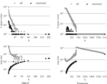
47 94 141 188 235 282 k 100 101 102 103 # span-cores all maximal 352 704 1056 1408 1760 2112 k 100 101 102 # span-cores all maximal DBLP Epinions

Figure 2: Top plots: number of all cores and maximal span-cores (y axis) as a function of the order k (x axis). Bottom plots: av-erage size of all span-cores and maximal span-cores (y axis) as a function of the orderk (x axis).

Characterization. We finally compare and characterize all cores against maximal cores. At first, Table 2 shows that span-cores are at least one order of magnitude more numerous than

maximal span-cores for all datasets, with the maximum difference of two orders of magnitude for theEpinions dataset.

In Figure 2 we show the number (top) and the average size (bottom) of span-cores and maximal span-cores as a function of the

orderk for the DBLP and Epinions datasets. For both datasets, the number of maximal span-cores is at least one order of magnitude lower than the total number of span-cores up to a quarter of the k domain, where the span-cores are more numerous. Instead, in the rest of the domain, they mostly coincide due to the maximality

condition over|∆|. The average size is also smaller for maximal span-cores, difference that wears thin when the gap between the

numbers of span-cores and maximal span-cores starts decreasing since, for high values ofk, most (or all) span-cores are maximal.

Figure 3 shows a different picture when numbers and average sizes are shown as a function of the size of the span|∆|. For both datasets, the number of span-cores and maximal span-cores

de-creases with, on average, a constant gap of one and two orders of magnitude, respectively, since the number of intervals decreases as |∆| increases. On the other hand, the behavior of the average size is quite different between the two datasets. For theDBLP dataset, the average size of span-cores is much higher than the average size of maximal span-cores for low values of|∆|, then the difference decreases and vanishes at the end of domain where a maximal

span-core of|∆| = 37 dominates all other span-cores of |∆| ≥ 20. Instead, for theEpinions dataset, the average size of all span-cores and maximal span-cores follows the same behavior, with a differ-ence of less than an order of magnitude, because the maximality

condition overk excludes the largest span-cores from the set of maximal span-cores.

6 12 18 24 30 36 | | 100 101 102 103 # span-cores all maximal 4 8 12 16 20 24 | | 100 101 102 103 104 # span-cores all maximal DBLP Epinions

Figure 3: Top plots: number of all cores and maximal span-cores (y axis) as a function of the size of the temporal span |∆| (x axis). Bottom plots: average size of all cores and maximal span-cores (y axis) as a function of the size of the temporal span |∆| (x axis).

7

APPLICATIONS

In this section we illustrate applications of (maximal) span-cores

in the analysis of face-to-face interaction networks. We use three datasets gathered by a proximity-sensing infrastructure with a

res-olution of 20 seconds. The first dataset, namedPrimarySchool2, contains the contact events between 242 individuals (232 children

and 10 teachers) in a primary school in Lyon, during two days [39]. TheHighSchool2dataset gives the interactions between students and teachers (327 individuals overall) of nine classes during five

days in a high school in Marseilles [30]. Finally, theHongKong dataset describes the interactions of people in a primary school in

Hong Kong for eleven consecutive days [35]. The school population consists of 709 children and 65 teachers divided into thirty classes.

For all three datasets we use a window size of 5 minutes and discard span-cores of|∆| = 1, i.e., having span of 5 minutes, since they represent extremely short group interactions, not significant for our purposes. On these datasets we show three types of interest-ing temporal patterns, i.e., social activities of groups of students

within a school day, mixing of gender and class, and length of social interactions in groups.

7.1

Temporal patterns

Temporal activity. We first show how span-cores yield a simple temporal analysis of social activities of groups of people within

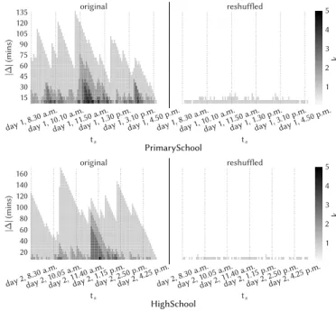
a school day. The left side of Figure 4 reports colormaps of the orderk of the span-cores as a function of their starting time t_s (x axis) and of the size of their temporal span|∆| (y axis), for a school day of thePrimarySchool and HighSchool datasets. Darker gray indicates span-cores of high order and slots located in the upper part of the plots refer to span-cores of long span. In both datasets, fluctuations ofk and |∆| are observed along the day, which can be

2

Available at sociopatterns.org.

day 1, 8.30 a.m.day 1, 10.10 a.m.day 1, 11.50 a.m.day 1, 1.30 p.m.day 1, 3.10 p.m.day 1, 4.50 p.m.

ts 15 30 45 60 75 90 105120 135 | ∆ | (m in s) original

day 1, 8.30 a.m.day 1, 10.10 a.m.day 1, 11.50 a.m.day 1, 1.30 p.m.day 1, 3.10 p.m.day 1, 4.50 p.m.

ts reshuffled 1 2 3 4 5 k PrimarySchool

day 2, 8.30 a.m.day 2, 10.05 a.m.day 2, 11.40 a.m.day 2, 1.15 p.m.day 2, 2.50 p.m.day 2, 4.25 p.m.

ts 20 40 60 80 100120 140 160 | ∆ | (m in s) original

day 2, 8.30 a.m.day 2, 10.05 a.m.day 2, 11.40 a.m.day 2, 1.15 p.m.day 2, 2.50 p.m.day 2, 4.25 p.m.

ts reshuffled 1 2 3 4 5 k HighSchool

Figure 4: Temporal activity of a school day of the PrimarySchool and HighSchool datasets: the x axis reports the hour of the day at which the span of a span-core starts, they axis specifies the size of the span (in minutes), and the color scale shows the orderk. At a glance, it can be observed that the temporal structure of the span-core decomposition detects time-evolving community structures in the original datasets (left plots) that completely disappears in the reshuffled datasets (right plots).

related to school events. Around 10 a.m., the size of the span|∆| reaches a local maximum in correspondence to the morning break,

which means that students establish long-lasting interactions that hold beyond the break itself. Moreover, when classes gather for the

lunch break, the orderk reaches its maximum value since students tend to form larger and more cohesive groups.

In order to verify that these results are not trivially derived from the general temporal activity, as simply given by the number of interactions in each timestamp, we compare our findings to a null

model. At each timestamp of the temporal graphs, we reshuffle the edges by repeating the following operations, up to when all

edges have been processed: select at random two edges with no common vertices, e.g.,(u,v) and (w, z), and transform them into (u, z) and (w,v). This reshuffling preserves degree of each vertex in each timestamp and global activity (i.e., number of contacts per

timestamp), but destroys correlations between edges of successive timestamps. In the right side of Figure 4 we show the results of the temporal analysis described above for the reshuffled datasets. In

both, the values of|∆| and k reached are much smaller than in the original datasets. The size of the span|∆| is always shorter than 20 minutes, while in the original datasets it is much longer, up to 170 minutes, and the orderk is always equal to 1, compared to the original maximum of 5. The time-evolving communities detected in the original datasets are completely lost after the reshuffling, where no temporal structure of the span-cores is observed. This proves

that the temporal schema of span-core decomposition is not simply a consequence of the overall activity but that span-cores represent

Figure 5:Temporal evolution (time on thex axis) of average gender purity and average class purity (y axis) of the maximal span-cores of the PrimarySchool dataset. Original data on the left, reshuffled data on the right.

Mixing patterns. We now show analysis of mixing patterns of students with respect to gender and class. Such metadata is indeed available for the individuals of thePrimarySchool dataset. We de-fine asgender purity of a span-core the fraction of individuals of the most represented gender within the span-core.Class purity is

analogously defined. The left plot of Figure 5 reports the temporal evolution of gender and class purity during the first school day of thePrimarySchool dataset: at each timestamp t , the curves rep-resent the average purities of the maximal span-cores spanningt. During lessons, when students are in their own classes, class purity

has naturally very high values, very close to 1. Gender purity is instead rather low. On the other hand, when students are gathered

together, during the morning break at 10 a.m. and the lunch break between 12 a.m. and 2 p.m., the situation is overturned: gender purity reaches large values while class purity drastically decreases.

This shows that primary school students group with individuals of the same class, disregarding the gender, only when they are forced

by the schedule of the lessons, but prefer to interact with students of the same gender during breaks, in agreement with a previous

study of the same dataset [38].

The right plot of Figure 5 shows the temporal evolution of gender

and class purity with gender and class randomly reshuffled among individuals. The two curves are more flat and the anti-correlation between them completely vanishes. This testifies that the results on

the original dataset are not simply due to the relative abundance of individuals of each type interacting at each time, but reflect genuine

mixing patterns over time.

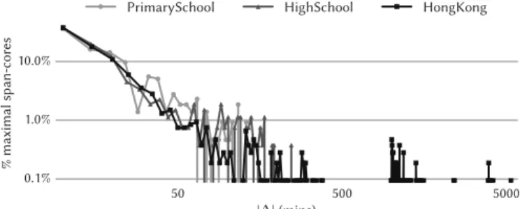
Interaction length. Finally, we analyze the duration of interac-tions of social groups in schools by studying the distribution of the

size of the span of the maximal span-cores of the three datasets (Fig-ure 6). All distributions are extremely skewed with broad tails: most

maximal span-cores have duration less than 1 hour, but durations much larger than the average can also be observed. Interestingly, similar functional shapes are shown by the three datasets,

confirm-ing a robust statistical behavior. We also note that similar robust broad distributions have been observed for simpler characteristics

of human interactions such as the statistics of contact durations [30, 39]. Outliers appear also at very large durations, especially for

theHongKong dataset that has maximal span-cores lasting up to 83 hours. Group interactions of such long span are clearly abnormal and represent outliers in the distributions. We will show, in the

50 500 5000 |∆| (mins) 0.1% 1.0% 10.0% % maximal span-cores

PrimarySchool HighSchool HongKong

Figure 6: Distribution of the size of the span |∆| of the maximal span-cores. Thex axis reports the size of the span (in minutes), while they axis the percentage of maximal span-cores having a given size of the span.

following of this section, how to exploit such outliers to detect both irregular contacts and anomalous temporal intervals.

7.2

Anomaly detection

The identification of anomalous behaviors in temporal networks

has been the focus of several studies in the last few years [32, 35]. Based on the above findings, we devise an extremely simple

proce-dure to detect anomalous contacts and intervals of theHongKong dataset that exploits maximal span-cores. The topmost plot of

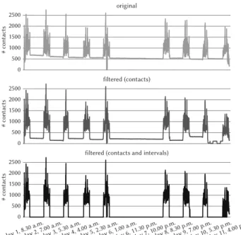
Fig-ure 7 reports the number of contacts, i.e., edges, for each timestamp of the originalHongKong dataset. It is easy to notice that there is a lot of constant anomalous activity between school days and during

the weekend, i.e., days six and seven. Unexpectedly, the number of contacts per timestamp does not drop to zero because proximity

sensors were left in each class, close to each other, at the end of the lessons. In order to automatically detect these steady activity

patterns, we apply the following procedure:(i) find a set of anoma-lously long temporal intervals supporting maximal span-cores,(ii) identify anomalous vertices, and,(iii) filter out anomalous contacts.

The first step of this procedure requires to find the set of temporal intervalsI= {∆ ⊑ T | C_k,∆∈C_M ∧ |∆| > tr } that are the span of a maximal span-coreC_k,∆with size longer than a certain threshold tr. Then, for each timestamp t ∈ T , select as anomalous all those vertices that appear in the span-cores{C1,∆ |∆ ∈ I ∧ t ∈ ∆}, i.e.,

the span-cores ofk = 1 whose span is in I and contains t. Finally, at each timestampt ∈ T , filter out the contacts having at least an anomalous endpoint at timet. Coherently to the distribution of the size of the span of the maximal span-cores, we select the threshold tr = 22 (110 minutes). The results of this filtering procedure are shown in the middle plot of Figure 7. The number of contacts

during school days remains substantially unchanged, while the activity noticeably decreases in-between. Identifying as positives

the contacts occurring when the school is closed and as negatives all the others (i.e., when the school is open), this approach achieves

a precision of 0.91 and a recall of 0.64.

We can refine this anomaly detection process by identifying, in addition to anomalous contacts, also anomalous temporal intervals.

We define a timestampt ∈ T as anomalous if the ratio between the number of original contacts (top plot of Figure 7) and the number of

filtered contacts (middle plot of Figure 7) exceeds a given threshold. We apply this further filtering to theHongKong dataset with a threshold of 1.5 and report the results in the bottommost plot of

Figure 7:HongKong dataset: number of contacts (y axis) per times-tamp (x axis) in the original data (top), after filtering anomalous contacts (middle), and after filtering anomalous contacts and inter-vals (bottom).

Figure 7. The number of contacts when the school is closed drops to zero, while the activity during school days is not modified, except

for the last one, which is affected by the proximity to the end of the time domain. The overall procedure yields a slightly higher value

of precision, 0.93, and substantially improves the recall to 0.99.

8

CONCLUSIONS

In this paper we introduced a notion of temporal core decompo-sition where each core is associated with its span, and developed efficient algorithms for computing all the span-cores, and only the

maximal ones. In our future work we will exploit span-cores for the computation of related notions, such ascommunity search or

densest subgraph in temporal networks. We will also study the role of maximal span-cores with large∆ in spreading processes on tem-poral networks. Furthermore, span-cores represent features that can be used for network finger-printing and classification, model

validation, and could provide support for new ways of visualizing large-scale time-varying graphs.

REFERENCES

[1] J. I. Alvarez-Hamelin et al. Large scale networks fingerprinting and visualization using the k-core decomposition. InNIPS, 2005.

[2] A. Angel et al. Dense subgraph maintenance under streaming edge weight updates for real-time story identification.PVLDB, 5(6), 2012.

[3] G. D. Bader and C. W. V. Hogue. An automated method for finding molecular complexes in large protein interaction networks.BMC Bioinformatics, 4:2, 2003. [4] V. Batagelj, A. Mrvar, and M. Zaversnik. Partitioning approach to visualization

of large graphs. InInt. Symp. on Graph Drawing, pages 90–97, 1999. [5] V. Batagelj and M. Zaveršnik. Fast algorithms for determining (generalized) core

groups in social networks.ADAC, 5(2), 2011.

[6] M. Berlingerio, F. Bonchi, B. Bringmann, and A. Gionis. Mining graph evolution rules. InECML PKDD 2009.

[7] F. Bonchi, I. Bordino, F. Gullo, and G. Stilo. Identifying buzzing stories via anomalous temporal subgraph discovery. InWI 2016.

[8] F. Bonchi, F. Gullo, A. Kaltenbrunner, and Y. Volkovich. Core decomposition of uncertain graphs. InKDD, 2014.

[9] B. Bringmann, M. Berlingerio, F. Bonchi, and A. Gionis. Learning and predicting the evolution of social networks.IEEE Intelligent Systems, 25(4):26–35, 2010. [10] J. Cheng, Y. Ke, S. Chu, and M. T. Özsu. Efficient core decomposition in massive

networks. InICDE, 2011.

[11] A. Das Sarma, A. Jain, and C. Yu. Dynamic relationship and event discovery. In WSDM 2011.

[12] E. Desmier, M. Plantevit, C. Robardet, and J.-F. Boulicaut. Cohesive co-evolution patterns in dynamic attributed graphs. InDS 2012.

[13] A. Epasto, S. Lattanzi, and M. Sozio. Efficient densest subgraph computation in evolving graphs. InWWW 2015.

[14] D. Eppstein, M. Löffler, and D. Strash. Listing all maximal cliques in sparse graphs in near-optimal time. InISAAC, 2010.

[15] P. Érdi et al.Prediction of emerging technologies based on analysis of the us patent citation network.Scientometrics, 95(1):225–242, 2013.

[16] E. Galimberti, F. Bonchi, and F. Gullo. Core decomposition and densest subgraph in multilayer networks. InCIKM 2017.

[17] A. Garas, F. Schweitzer, and S. Havlin. A k -shell decomposition method for weighted networks.New Journal of Physics, 14(8), 2012.

[18] D. Garcia, P. Mavrodiev, and F. Schweitzer. Social resilience in online communities: The autopsy of friendster.CoRR, abs/1302.6109, 2013.

[19] L. Gauvin, A. Panisson, and C. Cattuto. Detecting the community structure and activity patterns of temporal networks: a non-negative tensor factorization approach.PLOS ONE, 9(1):e86028, 2014.

[20] V. Gemmetto, A. Barrat, and C. Cattuto. Mitigation of infectious disease at school: targeted class closure vs school closure.BMC infectious diseases, 14(1):695, 2014. [21] C. Giatsidis, D. M. Thilikos, and M. Vazirgiannis. D-cores: measuring collaboration

of directed graphs based on degeneracy.KAIS, 35(2), 2013.

[22] J. Healy, J. Janssen, E. E. Milios, and W. Aiello. Characterization of graphs using degree cores. InWAW, 2006.

[23] A.-S. Himmel, H. Molter, R. Niedermeier, and M. Sorge. Enumerating maximal cliques in temporal graphs. InASONAM 2016.

[24] A. Inokuchi and T. Washio. Mining frequent graph sequence patterns induced by vertices. InSDM 2010.

[25] V. Jethava and N. Beerenwinkel. Finding dense subgraphs in relational graphs. InECML-PKDD 2015.

[26] M. Kitsak et al. Identifying influential spreaders in complex networks.Nature Physics 6, 888, 2010.

[27] G. Kortsarz and D. Peleg.Generating sparse 2-spanners.J. Algorithms, 17(2), 1994.

[28] C. W.-k. Leung, E.-P. Lim, D. Lo, and J. Weng. Mining interesting link formation rules in social networks. InCIKM 2010.

[29] R.-H. Li, J. X. Yu, and R. Mao. Efficient core maintenance in large dynamic graphs. IEEE Transactions on Knowledge and Data Engineering, 26(10):2453–2465, 2014. [30] R. Mastrandrea, J. Fournet, and A. Barrat. Contact patterns in a high school: A

comparison between data collected using wearable sensors, contact diaries and friendship surveys.PLoS ONE, 10(9):1–26, 09 2015.

[31] D. W. Matula and L. L. Beck. Smallest-last ordering and clustering and graph coloring algorithms.J. ACM, 30(3), 1983.

[32] M. Mongiovi et al. Netspot: Spotting significant anomalous regions on dynamic networks. InSDM 2013.

[33] A. Montresor, F. D. Pellegrini, and D. Miorandi. Distributed k-core decomposition. TPDS, 24(2), 2013.

[34] P. Rozenshtein, N. Tatti, and A. Gionis. Finding dynamic dense subgraphs.ACM Transactions on Knowledge Discovery from Data (TKDD), 11(3):27, 2017. [35] A. Sapienza et al. Detecting anomalies in time-varying networks using tensor

decomposition. InICDM Workshops 2015.

[36] A. E. Sariyüce, B. Gedik, G. Jacques-Silva, K. Wu, and Ü. V. Çatalyürek. Streaming algorithms for k-core decomposition.PVLDB, 6(6), 2013.

[37] K. Semertzidis, E. Pitoura, E. Terzi, and P. Tsaparas. Best friends forever (bff ): Finding lasting dense subgraphs.arXiv:1612.05440, 2016.

[38] J. Stehlé, F. Charbonnier, T. Picard, C. Cattuto, and A. Barrat. Gender homophily from spatial behavior in a primary school: A sociometric study.Social Networks, 35:604–613, 2013.

[39] J. Stehlé et al. High-resolution measurements of face-to-face contact patterns in a primary school.PLoS ONE, 6(8):e23176, 08 2011.

[40] T. Viard, M. Latapy, and C. Magnien. Computing maximal cliques in link streams. Theoretical Computer Science, 609:245–252, 2016.

[41] H. Wu, J. Cheng, Y. Lu, Y. Ke, Y. Huang, D. Yan, and H. Wu. Core decomposition in large temporal graphs. InBig Data (Big Data), 2015 IEEE International Conference on, pages 649–658. IEEE, 2015.

[42] S. Wuchty and E. Almaas. Peeling the yeast protein network.Proteomics, 5(2), 2005.

[43] H. Zhang, H. Zhao, W. Cai, J. Liu, and W. Zhou. Using the k-core decomposition to analyze the static structure of large-scale software systems.J. Supercomputing, 53(2), 2010.