A Maxwell-Elasto-Brittle model for the drift and deformation of sea ice

HAL Id: tel-01316987

https://tel.archives-ouvertes.fr/tel-01316987

Submitted on 17 May 2016

HAL is a multi-disciplinary open access

archive for the deposit and dissemination of

sci-entific research documents, whether they are

pub-lished or not. The documents may come from

teaching and research institutions in France or

abroad, or from public or private research centers.

L’archive ouverte pluridisciplinaire HAL, est

destinée au dépôt et à la diffusion de documents

scientifiques de niveau recherche, publiés ou non,

émanant des établissements d’enseignement et de

recherche français ou étrangers, des laboratoires

publics ou privés.

A Maxwell-Elasto-Brittle model for the drift and

deformation of sea ice

Véronique Dansereau

To cite this version:

Véronique Dansereau. A Maxwell-Elasto-Brittle model for the drift and deformation of sea ice.

Me-chanics [physics]. Université Grenoble Alpes, 2016. English. �NNT : 2016GREAU003�. �tel-01316987�

TH `ESE

Pour obtenir le grade de

DOCTEUR DE LA COMMUNAUT ´E

UNIVERSIT ´E GRENOBLE ALPES

Sp´ecialit´e : Sciences de la Terre et de l’Univers et de l’Environnement

Arrˆet´e minist´eriel : 7 Aoˆut 2006

Pr´esent´ee par

V´eronique Dansereau

Th`ese dirig´ee par J´er ˆome Weiss

et codirig´ee par Pierre Saramito

pr´epar´ee au sein du

Laboratoire de Glaciologie et G´eophysique de l’Environnement

dans l’ ´Ecole Doctorale Terre Univers Environnement

Un mod`ele Maxwell-´elasto-fragile pour

la d´eformation et d´erive de la banquise

Th`ese soutenue publiquement le 17 F´evrier 2016,

devant le jury compos´e de :

Mme Anne Mangeney

Professeur, Universit´e Paris Diderot/IPGP, Pr´esidente et Rapporteur

M. Vincent Legat

Professeur, Universit´e Catholique/ ´Ecole Polytechnique de Louvain, Rapporteur

M. Franc¸ois Renard

Professeur, Universit´e Grenoble Alpes/ISTerre, Examinateur

Mme Annie Audibert-Hayet

Direction Scientifique, Comit´e Technologie Groupe TOTAL S.A., Examinatrice

M. J´er ˆome Weiss

Directeur de recherche, CNRS - Institut des Sciences de la Terre, Directeur de th`ese

M. Pierre Saramito

Directeur de recherche, CNRS - Laboratoire Jean Kuntzmann, Co-Directeur de th`ese

A Maxwell-Elasto-Brittle model

for the drift and deformation of sea ice

Acknowledgements - Remerciements

I am writing this page as the last of this thesis. Yet I feel it is the most important one.

I would like to thank J´erˆome, first for o↵ering me the opportunity to come to Grenoble and work on this

Ph.D. project. This opportunity came as a surprise; unplanned. The work, as the life here, has been chal-lenging in many ways. But most importantly, it has been even more stimulating than I hoped it to be. Hence saying that I am thankful for the role he played in this unexpected turn of events is simply an understatement. Second, I would like to thank him for his support. And by support I mean more than correcting me for the inadequate use of the word ”constraint” a thousand times.

The second person I would like to thank is Pierre, for his precious advices, his contagious enthusiasm and his never-failing patience in answering my multiple, slightly bewildered or completely confused, math questions. I am also grateful for the support I received and stimulating contacts I had with many people at Total. I especially thank Annie Audibert-Hayet, Edmond Coche, Philippe Lattes, Philippe Ricoux and Kaj Riska for their valuable suggestions on this work and their many encouragements.

I thank my reviewers, Anne Mangeney and Vincent Legat, as well as my examinators, Annie Audibert-Hayet and Fran¸cois Renard for their time and their numerous, useful advices.

Then let me just make a list of the people I would like to express my gratitude to, although simply list-ing their names does not really pay justice to my appreciation of their presence and help:

Anne-Marie Cˆot´e, Elizabeth Cˆot´e, everyone at Coll`ege Rivier, Daniel L´eveill´e, Pascaline, Elsa, H´el`ene, Marion, Soazig, Alban, Isabelle, Sarah, Cracou, Nikki, Arnaud, Francois, Johanna, Pauline, Quentin, Yoann, Nelly, St´ephane, Mathias, David, Lucas, Jonathan,

Maurine, Fred, Bruno, Xue Meng, Mara, Francois, Audrey, Gabi, Ad`ele,

Mimi, Mamie, Papi.

Abstract

In recent years, analyses of available ice buoy and satellite data have revealed the strong heterogeneity and intermittency of the deformation of sea ice and have demonstrated that the viscous-plastic rheology widely used in current climate models and operational modelling platforms does not simulate adequately the drift, deformation and mechanical stresses within the ice pack.

A new alternative rheological framework named Maxwell-Elasto-Brittle (Maxwell-EB) is therefore developed here in the view of reproducing more accurately the drift and deformation of the ice cover in continuum sea ice models at regional to global scales. The model builds on an elasto-brittle framework used for ice and rocks. A viscous-like relaxation term is added to a linear-elastic constitutive law together with an e↵ective viscosity that evolves with the local level of damage of the material, like its elastic modulus. This framework allows for part of the internal stress to dissipate in large, permanent deformations along the faults/leads once the material is highly damaged while retaining the memory of small, elastic deformations over undamaged areas. A healing mechanism is also introduced, counterbalancing the e↵ects of damaging over large time scales.

The numerical scheme for the Maxwell-EB model is based on finite elements and variational methods. The equations of motion are cast in the Eulerian frame and discontinuous Galerkin methods are implemented to handle advective processes.

Idealized simulations without advection are first presented. These demonstrate that the Maxwell-EB rhe-ological framework reproduces the main characteristics of sea ice mechanics and deformation : the strain localization, the anisotropy and intermittency of deformation and the associated scaling laws. The successful representation of these properties translates into very large gradients within all simulated fields. Idealized nu-merical experiments are conducted to evaluate the amount of nunu-merical di↵usion associated with the advection of these extreme gradients in the model and to investigate other limitations of the numerical scheme. First large-deformation simulations are carried in the context of a Couette flow experiment, which allow a comparison with the result of a similar laboratory experiment performed on fresh-water ice. The model reproduces part of the mechanical behaviour observed in the laboratory. Comparison of the numerical and experimental results allow identifying some numerical and physical limitations of the model in the context of large-deformation and laboratory-scale simulations. Finally, the Maxwell-EB framework is implemented in the context of modelling the drift and deformation of sea ice on geophysical scales. Idealized simulations of the flow of sea ice through a narrow channel are presented. The model simulates the propagation of damage along arch-like features and successfully reproduces the formation of stable ice bridges.

Keywords : sea ice deformation, Maxwell-elasto-brittle rheology, brittle mechanics, elastic interactions, viscous stress relaxation, heterogeneity, intermittency, anisotropy, finite elements and discontinuous Galerkin methods.

R´

esum´

e

Depuis quelques ann´ees, des analyses statistiques de donn´ees satellitales et de bou´ees d´erivantes ont r´ev´el´e le caract`ere hautement h´et´erog`ene et intermittent de la d´eformation de la banquise Arctique, d´emontrant de ce fait que le sch´ema rh´eologique visco-plastique traditionellement utilis´e en mod´elisation climatique et op´erationnelle ne simule pas ad´equatement le comportement dynamique des glaces ainsi que les e↵orts m´ecaniques en leur sein.

Un cadre rh´eologique alternatif, baptis´e Maxwell- ´Elasto-Fragile (Maxwell-EB) est donc ici d´evelopp´e dans le but de reproduire correctement la d´erive et la d´eformation des glaces dans les mod`eles continus de la banquise `a l’´echelle r´egionale et globale. Le mod`ele se base en partie sur un cadre de mod´elisation ´elasto-fragile utilis´e pour les roches et la glace. Un terme de relaxation visqueuse est ajout´e `a la relation constitutive d’´elasticit´e lin´eaire avec une viscosit´e e↵ective, ou ”apparente”, laquelle ´evolue en fonction du niveau d’endommagement local du mat´eriel simul´e, comme son module d’´elasticit´e. Ce cadre rh´eologique permet la dissipation partielle des contraintes internes par le biais de d´eformations permanentes, possiblement grandes, le long de failles (ou ”leads”) lorsque le mat´eriel est fortement endommag´e ainsi que la conservation de la m´emoire des contraintes

associ´ees aux d´eformations ´elastiques dans les zones o`u le mat´eriel reste relativement peu endommag´e. Un

m´ecanisme de cicatrisation permettant de repr´esenter le regel le long des failles form´ees est ´egalement inclus. The sch´ema num´erique du mod`ele Maxwell-EB est bas´e sur des m´ethodes de calcul variationnel et par ´el´ements finis. Une repr´esentation Eul´erienne des ´equations du mouvement est utilis´ee et des m´ethodes dites Galerkin discontinues sont impl´ement´ees pour le traitement des processus d’advection.

Une premi`ere s´erie de simulations id´ealis´ees et sans advection est pr´esent´ee, lesquelles d´emontrent que la rh´eologie Maxwell-´Elasto-Fragile reproduit les caract´eristiques principales du comportement m´ecanique de la banquise, c’est-`a-dire la localisation spatiale, l’anisotropie et l’intermittence de sa d´eformation ainsi que les lois d’´echelle qui en d´ecoulent. La repr´esentation ad´equate de ces propri´et´es se traduit par la pr´esence de tr`es forts gradients au sein des champs de contrainte, de d´eformation et du niveau d’endommagement simul´es par le mod`ele. Des tests visant `a ´evaluer la di↵usion num´erique d´ecoulant de l’advection de ces gradients extrˆemes ainsi qu’`a identifier certaines contraintes num´eriques du mod`ele sont ensuite pr´esent´es. De premi`eres simulations en grandes d´eformations, incluant les processus d’advection, sont r´ealis´ees, lesquelles permettent une comparaison aux r´esultats d’une exp´erience de Couette annulaire sur de la glace fabriqu´ee en laboratoire. Le mod`ele reproduit en partie le comportement m´ecanique observ´e. Par ailleurs, les di↵´erences entre les r´esultats des simulations et ceux obtenus en laboratoire permettent d’identifier certaines limitations, num´eriques et physiques, du mod`ele en grandes d´eformations. Finalement, le mod`ele rh´eologique est utilis´e pour mod´eliser la d´erive et la d´eformation des glaces `a l’´echelle de la banquise Arctique. Des simulations id´ealis´ees de l’´ecoulement de glace dans un chenal ´etroit sont pr´esent´ees. Le mod`ele simule une propagation localis´ee de l’endommagement, d´efinissant des failles en forme d’arche, et la formation de ponts de glace stables.

Mots-cl´es : d´eformation de la banquise, rh´eologie Maxwell-´elasto-fragile, m´ecanique fragile, interactions ´elastiques, relaxation visqueuse des contraintes, h´et´erog´en´eit´e, intermittence, anisotropie, m´ethodes de calcul par ´el´ements finis et Galerkin discontinues.

Table of Contents

1 Introduction 1

1.0.1 Context . . . 1

1.0.2 The Elasto-Brittle approach . . . 4

1.0.3 The small and large deformations of sea ice . . . 5

1.0.4 A finite element sea ice model . . . 8

1.0.5 Composition of the dissertation . . . 10

2 A Maxwell-Elasto-Brittle rheology for sea ice modelling 12 2.1 The building of a viscous-elastic-brittle continuum model . . . 13

2.1.1 Towards a Maxwell-Elasto-Brittle rheology . . . 14

2.1.2 Bridging small and large deformations . . . 15

2.2 The Maxwell-EB model . . . 17

2.2.1 Damage criterion . . . 17

2.2.2 Disorder . . . 18

2.2.3 Progressive damage mechanism and healing . . . 20

2.2.4 Characteristic numbers and times . . . 26

2.3 Small-deformation simulations . . . 31

2.3.1 Numerical scheme : the small-deformation Maxwell-EB model . . . 34

2.4 Results . . . 40

2.4.1 Spatial resolution, convergence and dependence on the initial conditions . . . 40

2.4.2 Heterogeneity . . . 42

2.4.3 Intermittency . . . 45

2.5 Sensitivity analyses . . . 48

2.6 Concluding remarks . . . 54

3 Towards a large-deformation Maxwell-EB model 56 3.1 From small to large deformations in the Maxwell-EB framework . . . 56

3.2 Advection and di↵usion . . . 60

3.2.1 P0approximations . . . 63

3.2.2 Higher order FE approximations . . . 64

3.3 Rotation and deformation . . . 67

3.3.1 Numerical scheme . . . 68

3.3.2 Stationary solution . . . 72

3.4.1 Laboratory Couette experimental setup . . . 75

3.4.2 Numerical Couette experiment setup . . . 75

3.4.3 Numerical scheme : the large-deformation Maxwell-EB model . . . 78

3.4.4 A comparison of Couette experiments . . . 84

3.4.5 Discussion . . . 91

3.5 Concluding remarks . . . 93

4 A Maxwell-EB sea ice model 95 4.1 A realistic case study . . . 95

4.2 The complete picture . . . 98

4.3 Channel flow simulations . . . 99

4.4 Numerical scheme . . . 102

4.4.1 Time discretization . . . 103

4.4.2 Variational formulation and discontinuous Galerkin FE approximation . . . 105

4.5 Results . . . 109

4.5.1 Dynamical behavior . . . 109

4.5.2 Ice thickness and concentration . . . 116

4.6 Concluding remarks . . . 119

5 Conclusions 122 5.1 A brief summary . . . 122

5.2 Some perspectives . . . 124

5.2.1 Towards a fully continuous formulation of the Maxwell-EB rheology . . . 124

5.2.2 Future developments and additions to the rheology . . . 126

Chapter 1

Introduction

1.0.1

Context

The ice that covers the polar oceans moves and deforms under the action of the winds and ocean currents. Making reliable predictions of the drift and deformation of this thin floating sheet of ice is becoming crucial nowadays for: (1) forecasting the opening of shipping routes across the Arctic, (2) evaluating mechanical constraints on o↵shore structures and ships and, at larger scales, (3) estimating the future evolution of both its summer and winter extent in the Arctic and Antarctic to anticipate its short to long-term, regional to global impacts on climate.

Early aerial pictures of the Arctic ice cover have revealed a highly heterogeneous, ”densely fractured ma-terial” (Coon et al., 1974), divided in plates, called ”floes”, of sizes ranging from a few meters to several kilometres (see figure 1.1). The relative motion of these floes translates into the opening of cracks, joining along larger features called ”leads”, the shearing deformation along opened cracks, the closing of leads and the formation of pressure ridges (Coon et al., 1974; Feltham, 2008; Weiss, 2013, and others). In more recent years, satellite remote sensing data such as the RADARSAT Geophysical Processor System sea ice motion products have allowed observing the strong localization of the deformation of sea ice along linear features, termed ”linear kinematic features” (Kwok, 2001), which corresponds to active faults within the ice cover and the associated discontinuities in the drift velocities (see figure 1.2).

From the modelling point of view, the approach that appears the most natural to represent the dynamics of the ice cover at the scale of an aggregate of a few floes (see figure 1.1) is one in which individual ice plates are resolved and floe-to-floe interactions are treated explicitly. Discrete element-type methods have indeed been recently developed to model the mechanics and kinematics of sea ice at these small scales (e.g. Hopkins, 2004; Herman, 2011; Wilchinsky et al., 2011; Rabatel et al., 2015). In the context of long-term and global scale simulations of the sea ice cover, such models however remain computationally too expensive. As in general they do not handle fracturing processes within the floes, they are also better suited for the representation of a low concentration ice cover (< 80%) than of a dense ice pack. Current regional and global climate models as well as most operational modelling platforms are instead based on a continuum mechanics description of sea ice. Besides computational efficiency, this approach presents the advantage of being more suitable for a coupling with atmosphere and ocean models. In this case the motion of the thin ice cover is described by a

Space (m) Individual floes 100 ₁₀1 ₁₀2 ₁₀4 ₁₀5 ₁₀6

Tim

e

Sea ice cover

(

Figure 1.1: Areal pictures of sea ice (from bottom to top) at the scale of 100 meters,_{⇠ 5 km and 60 km. At the smallest} time and space scales, the discontinuous nature of the ice cover cannot be ignored when modelling its deformation and drift. At large scales ( 104 _{m), the ice cover is constituted by a large number of individual ice floes of di↵erent shapes}

and sizes and is described by mean quantities in continuum models.

two-dimensional Navier-Stokes-type equation of the form ⇢h

_@u

@t + (u· r)u = Fext+r · (h ), (1.1)

with ⇢ the density, u the mean velocity, h the mean thickness of the ice and Fext, the external forces on the

ice cover, typically the air and ocean drags, the Coriolis force and the sea surface tilt. The last term in this momentum balance equation stands for the mean internal force that arises from the sum of all mechanical interactions between ice floes. Without a treatment of the kinematics of the discrete floes or individual leads, the relationship between the corresponding internal stress tensor, , and the macroscopic deformation of the ice cover must be prescribed through a rheological law. Perhaps the biggest challenge of the continuum mod-elling approach lies in the formulation of this constitutive law (Feltham, 2008), which must allow representing adequately through mean quantities a material with a inherently discontinuous character.

Current operational modelling platforms, whether assimilating data or not (e.g., TOPAZ4 : Sakov et al. (2012), GIOPS : Smith et al. (2015)), and global climate models including sea ice dynamics (e.g., the Coupled Model Intercomparison Project Phase 5 models involved in the IPCC Fifth Assessment Report (Flato et al., 2013)) are based on the same rheological framework for sea ice developed in the late seventies: the Hibler Viscous-Plastic (VP) model (Hibler, 1977, 1979). With this approach, the ice creeps very slowly as a viscous fluid under small stresses and deforms plastically once exceeding a yield criterion. Yet, over the last decade, the viscous hypothesis and other underlying physical assumptions of this VP framework have been revisited

Figure 1.2: Weekly fields of divergence (upper left), vorticity (middle left), shear (lower left) and sea ice mo-tion (x-component, y-component and magnitude) for the period of February 8 to February 14 2008 over the Arc-tic basin, showing the concentration of deformation within linear features and clear discontinuities in the velocity field. The fields are estimated from the 3-days RADARSAT Geophysical Processor System sea ice motion products (http://rkwok.jpl.nasa.gov/graphics/index.html)

and found inconsistent with the observed mechanical behaviour of sea ice (Weiss et al., 2007; Coon et al., 2007; Rampal et al., 2008). In the same line of ideas, recent modelling studies have demonstrated that while the

VP model can represent with a certain level of accuracy the mean, global (> 100 km) drift of sea ice, it fails at reproducing the observed properties of sea ice deformation and that, especially at the fine scales (Lindsay et al., 2003; Kwok et al., 2008; Girard et al., 2009) relevant for operational modelling, thereby stressing the need to explore alternative rheologies.

Other modelling frameworks have been developed lately with the aim of representing more accurately some important aspects of the mechanical behaviour of sea ice. Considering the discontinuous and anisotropic character of the pack, Schreyer et al. (2006) have suggested an elastic-decohesive model that explicitly accounts for the deformation arising from discontinuities in displacements across leads, the orientation of which is prescribed. Tsamados et al. (2013) have presented a continuum model based on the rheology of Wilchinsky and Feltham (2006) that accounts for the subgrid scale anisotropy of the sea ice cover. Their framework incorporates an evolution equation for the orientation of ice floes, for which a diamond shape is assumed. Our present work shares the same objective as these previous initiatives: to build a continuum model for sea ice that is physically consistent with its observed mechanical behaviour. However, we chose to base our approach on a completely isotropic rheology and, by incorporating the relevant brittle mechanics concepts and long-range elastic interactions, aim to develop a model that reproduces the anisotropy and extreme gradients within the sea ice cover naturally, that is, without the need of treating velocity discontinuities explicitly nor prescribing lead orientations or floe shapes.

1.0.2

The Elasto-Brittle approach

Early on, sea ice scientists have suspected that the sea ice cover behaves in a brittle instead of a viscous manner, with some strain hardening in compression (Nye, 1973). Studies of fracture patterns, stresses and strains both in situ and in the laboratory have suggested that the deformation of sea ice is mostly accommodated by a mechanism of multiscale fracturing and frictional sliding (Marsan et al., 2004; Schulson, 2006a; Schulson and Duval, 2009; Weiss et al., 2007; Weiss and Schulson, 2009). By investigating the dispersion of ice buoys over the Arctic, Rampal et al. (2008) recently showed that sea ice deforms in a heterogenous and intermittent manner over spatial scales of 300 m to 300 km and time scales of 3 hrs to 3 months. The strong space-time coupling in the scaling laws revealed by their analyses are consistent with (1) a brittle-type material in which permanent deformations are accommodated by displacements along fractures and fault planes over a wide range of scales and (2) long-range elastic interactions, allowing for small, local perturbations to trigger much larger damaging events within the ice pack (Marsan and Weiss, 2010). The form of the scaling laws itself implies that the spatial heterogeneity and intermittency characterizing sea ice deformation decrease very slowly when increasing the scale of observation and therefore indicates that even at large scales, averaging the mechanical properties and deformation rates of the Arctic sea ice does not give rise to a smooth, possibly viscous-like behaviour as suggested by Hibler (1977).

A close comparison can be made between the deformation of sea ice and that of the Earth crust, in which brittle fracturing and Coulomb stress redistribution also take place and for which scaling properties have been recognized for years (Kagan and Knopo↵, 1980; Kagan, 1991; Kagan and Jackson, 1991; King et al., 1994; Turcotte, 1992; Stein, 1999). Recently, Marsan and Weiss (2010) established a formal analogy between the mechanical behaviour of sea ice and the Earth crust by demonstrating that the space-time coupling in the deformation of sea ice, estimated from continuous displacement fields, is equivalent to a coupled scaling of the discrete ice-fracturing events occurring along the leads, similar to that observed for earthquakes (Kagan, 1991; Kagan and Jackson, 1991). The authors suggested that the similarity between sea ice and the Earth crust is

attributable to a common cascading mechanism of earth-/ice-fracturing events that extends the influence of local events to longer durations and larger areas than their direct aftershocks.

In the case of rocks, attempts to simulate brittle deformation were first made using random spring-like models. Combining local threshold mechanics and long-range elastic interactions, these successfully reproduced the strong localization of rupture in both space and time, the clustering of rupture events along faults and the multifractal properties of strain fields (Cowie et al., 1993, 1995). Building on similar linear-elastic laws and introducing some strain softening at the micro scale, the failure model of Tang (1997) succeeded in simulating the progressive failure leading to the macroscopic non-linear behaviour of brittle rock, thereby processing discontinuum mechanics by a continuum mechanics method. An analogous approach based on local damage evolution was also taken by Amitrano et al. (1999), who combined

• a linear-elastic constitutive law for a continuum solid, • a local Mohr-Coulomb criterion for brittle failure,

• an isotropic progressive damage mechanism for the elastic modulus described by a non-dimensional scalar damage parameter, allowing for the redistribution of the stress from over-critical to sub-critical areas of the material, for the triggering of avalanches of damaging events and the propagation of faults.

Their model was shown to reproduce macroscopic brittleness and scaling laws in the distribution of damage events, consistent with earthquake observations (Amitrano, 2003).

In light of the analyses of sea ice deformation of Marsan et al. (2004); Weiss et al. (2007); Rampal et al. (2008) and others and of the similarity between the mechanical behaviour of sea ice and that of the Earth crust emphasized by Marsan and Weiss (2010), this rheological framework, named Elasto-Brittle (EB) was recently developed in the context of the Arctic ice pack by Girard et al. (2010b) to explicitly introduce brittle mechanics concepts in continuum sea ice models. First implementations of this rheology into short (3-days), no-advection, stand-alone simulations of the Arctic pack, but using realistic wind forcing from reanalyses, showed that a Lagrangian EB model is able to reproduce the strong spatial localization and the anisotropy of damage within sea ice and to simulate deformation fields in good agreement with that reconstructed from the RADARSAT Geophysical Processor System (RGPS) ice motion data (Girard et al., 2010b).

1.0.3

The small and large deformations of sea ice

In the context of longer-term simulations of ice conditions and coupling to an ocean component, a suitable sea ice model needs to represent not only the small deformations associated with the fracturing of the ice pack, but also the permanent deformations occurring once the pack is fragmented and ice floes move relative to each other along open leads, as these much larger deformations set the advective processes and overall drift pattern of the ice cover.

This point is an important and intrinsic limitation of the EB framework. To illustrate this limitation, let us represent schematically a linear-elastic and damageable material by a spring, with one free end and an initially

undamaged elastic modulus E0_{, as shown in figure 1.3a. Let us further consider that the maximum stress this}

material (i.e., the spring) can sustain without being structurally damaged is c. If a stress, , smaller than

c, is applied at time t, the resulting deformation of the spring, " is purely elastic and directly proportional to

the stress, as shown on figure 1.3b (dotted line). Conversely, if > c, the spring becomes damaged, which

translates into a diminution of its elastic modulus E and a non-linear deformation (figure 1.3b, solid black curve).

1

t

2

"

"

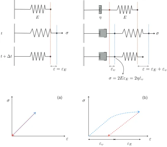
Figure 1.3: (a) Schematic representation of the Elasto-Brittle model, which combines a linear elastic constitutive law and a progressive damage mechanism. At time t, an overcritical stress, > c, is applied to the system. It is removed at

time t + t. In the all-elastic deformation assumption case (1), the damaged spring goes back to its initial position when the loading is removed. In the all-permanent deformation assumption case (2), it keeps its final position. In both cases, the damaged spring has a degraded elastic modulus, E < E0_{. (b) Stress-strain diagram for the linear elastic (dotted}

black line) and EB (solid and dashed lines) model. The black dot indicates the onset of damaging in the EB model, after which the model behaviour diverges from the linear-elastic case. The dashed red unloading path corresponds to the all-elastic deformation limit (1) and the dashed purple unloading path, to the all-permanent deformation limit (2).

Because its structure has been damaged, if the spring is released at time t + t, it is not expected to go

back to its exact initial position. Instead, part of its deformation is expected to remains permanent. Yet, if the deformation of the spring is modelled using a linear-elastic constitutive law, i.e., Hooke’s law, as is the Elasto-Brittle framework (Amitrano et al., 1999; Girard et al., 2010b), the model will solve for its total deformation " : it will not distinguish between the elastic (recoverable) and the potentially permanent part of its deformation. Hence to estimate the deformation rate (i.e., the velocity) of a damaged elastic material in such a model, assumptions about the amount of reversible versus irreversible deformation must be made. The partitioning is bounded by two limit cases, which can be illustrated using the same linear spring system (see figure 1.3a).

1. If all of the deformation of the damaged material (spring) is assumed elastic, whatever its damage level, the material goes back to its initial position when unloaded (figure 1.3a, case 1) as represented by the red, dashed unloading path on figure 1.3b. The elastic modulus of the material is degraded, but its velocity in this case is zero. This assumption was made by Girard et al. (2010b), who neither updated the position of mesh element nodes nor estimated advection processes in their Lagrangian, short-term simulations of the Arctic sea ice cover.

2. If all of the deformation of the material is considered permanent, the material always keeps its final position when unloaded (see figure 1.3a, case 2 and figure 1.3b, purple dashed unloading path). In this case, velocities and deformation rates can be trivially estimated as the ratio of the total deformation and of the time associated with the loading process ( t).

deformations within an undamaged ice pack are small compared to the permanent deformations associated with the opening, closing, and shearing along leads. Considering an undamaged elastic modulus between 1.0

and 10.0_{· 10}9_{Pa (Timco and Weeks, 2010), the maximum in-situ values of shear stress of 10}5_{Pa reported by}

Weiss et al. (2007) and a time scale for these stress measurements of 1 day, upper bound values for daily shear

strain rates in a one meter thick, purely elastic ice pack would be on the order of 10 5 _day 1_{. This is less}

than the lower bound deformation rate estimates from RGPS data (between 10 4 _{and 10}0_day 1_{, for Marsan}

et al. (2004); Girard et al. (2009)), suggesting a dominant contribution of irreversible deformations. This assumption is taken in the recently developed neXtSIM sea ice model, which is based on the EB rheology and does estimate advective processes over the Arctic (Bouillon and Rampal, 2015; Rampal et al., 2015). However in the all-permanent deformations limit, internal stresses are instantaneously dissipated in the damaged material. Hence the memory of the stresses associated with elastic deformations is erased whenever the applied loading is removed or reset. Without carrying this history of previous stresses, the model cannot reproduce the intermittency intrinsic to the mechanical behaviour of the material. In the context of sea ice modelling, this implies that the model only reproduces the part of the intermittency that is inherited from fluctuations of the wind forcing and cannot represent the observed long-range temporal correlations and extreme fluctuations in the deformation that emanate from elastic interactions within the ice cover (Weiss, 2008; Rampal et al., 2008). In order to represent the observed properties of the deformation of sea ice and estimate adequate drift velocities, a suitable rheological model must therefore have the capability to distinguish between reversible and irreversible deformations.

The goal of this work is to develop such a model allowing a transition from the small/elastic to the large/permanent deformations and with the capability of damage mechanics models to reproduce the ob-served space and time scaling properties of sea ice deformation. Our approach consists in introducing a viscous relaxation term into the linear-elastic constitutive law of the original EB framework. The new constitutive law takes the form of the Maxwell viscoelastic model. The all-important di↵erence with respect to the Maxwell framework however is that the viscosity associated with the stress dissipation term is not meant to represent the viscoplastic creep of bulk ice (Duval et al., 1983). Instead, it is an ”apparent” viscosity which, like the elastic modulus in the Elasto-Brittle framework, is coupled to the level of damage of the ice cover and allowed to evolve in both space and time according to a progressive damage mechanism. The coupling is designed so that strains remain elastic over undamaged portions of the ice and are dissipated through permanent deformations where the pack is highly fractured.

The use of a viscoelastic rheology and apparent viscosity in the case of sea ice can be supported again by the similarity between the mechanical behaviour of the ice pack and that of the Earth crust and by the existence of similar approaches to model lithospheric faulting. Active faults in the Earth crust have been known to deform in two distinct manners: either abruptly, causing earthquakes, or in a transient, aseismic manner (Scholz, 2002; Gratier et al., 2014; Cakir et al., 2012; Cetin et al., 2014). Similar to sea ice, co-seismic fracturing activates aseismic creep, leading to deformations that can be much larger than that associated with the fracturing itself (Cakir et al., 2012; Cetin et al., 2014) and to slip rates that decrease progressively over years to decades due to various healing processes (Gratier et al., 2014). Recent studies on aseismic faults (e.g., the Izmit fault) have suggested that creep relaxes a significant amount of elastic strain along the fault, retarding stress accumulation along some portions (and concentrating stresses on other locked portions), thereby demonstrating that this dissipative process needs to be included in earthquakes models (Cakir et al., 2012; Gratier et al., 2014).

A further justification of the introduction of such pseudo-viscosity comes from the rheology of granular media. As sea ice along leads (see figure 2.5), rocks along active faults are highly fragmented. Sheared granular

media flow in a viscous manner when inertial e↵ects can be neglected (Jop et al., 2006) with an apparent viscosity diverging as the packing fraction approaches the closed-packed limit (Aranson and Tsimring, 2006). This last point will justify the dependence of our apparent viscosity on sea ice concentration.

Viscous-elastic rheological models using apparent viscosities have already been used to model the defor-mation of rock-like materials. Lyakhovsky et al. (1997) built a viscoelastic damage rheology model with the intent of representing the di↵erent stages of geological faulting, from subcritical crack growth to increasing crack concentration and material degradation, macroscopic brittle failure, post failure deformation and heal-ing. Their progressive damage mechanism involved a scalar variable similar to that used in the EB and our Maxwell-EB framework, but the evolution of damage in their model was derived from energy conservation principles rather than from a brittle failure criterion and was coupled to the elastic modulus only. Frederiksen and Braun (2001) successfully simulated strain localization during lithospheric extension using an elasto-visco-plastic model together with an ad hoc viscosity. As their work was concerned with the ductile rather than the brittle deformation regime, strain softening in their model did not involve a progressive damage mechanism but instead was achieved by coupling the viscosity to the accumulated strain and the elastic modulus of the material was kept constant. Hamiel et al. (2004) modified the coupled linear elasticity and progressive damage rheological framework of Lyakhovsky et al. (1997) with a non-linear damage-elastic moduli relation and by adding a damage-dependent Maxwell-like viscous term (with the damage still evolving according to energy conservation) to account for the gradual accumulation of irreversible strain observed in typical rock mechanics experiments. Doing so they obtained better agreement with the observed deformation near the peak loading stress preceding the macroscopic failure of rock samples. The use of a viscous relaxation term in their rheo-logical framework therefore had a fundamentally di↵erent purpose than in the present approach in that it was intended for the representation of small, pre-macroscopic brittle failure deformations, not to bridge between small and large deformations.

To our knowledge, it is therefore the first time a viscoelastic Maxwell constitutive law is coupled to a progressive damage (and healing) mechanism through both the elastic modulus and an apparent viscosity with the intent of reproducing the small deformation associated with brittle fracturing and the large, permanent post-fracture deformation of geomaterials. It is certainly the first time such a rheological model has been adapted in the context of sea ice modelling.

1.0.4

A finite element sea ice model

In terms of formulating the discrete approximation of the equations of motion, finite element (FE) are known for the ease with which they can handle structured or unstructured meshes, complex geometries, boundary conditions, interface conditions and material properties. Although the relevance of these methods in the context of sea ice modelling were recognized as early as the 1970’s Arctic Ice Dynamics Joint Experiment (AIDJEX) (Becker, 1976), finite di↵erences (FD) have been common practice among the sea ice community due to the practicality of regular grids and because of their widespread use in ocean and climate models.

In late years, significant e↵orts have been put into incorporating FE methods in sea ice and ocean general circulation models in order to take advantage of multi-resolution mesh grids and better resolve complex flows with local phenomenons. In 2004, Wang and Ikeda presented a FE formulation for a dynamical sea ice model based on the Hibler VP rheology and proved their numerical scheme to be both stable and efficient. Lietaer et al. (2008) developed a large-scale FE sea ice model, operational for climate studies and destined to be coupled to the FE Second-generation Louvain-la-Neuve Ice-ocean Model (SLIM, http://www.climate.be/SLIM). They tested

their unstructured grid approach and investigated the sensitivity of the simulated thickness of Arctic sea ice to the resolution of the narrow, intricate straits of the Canadian Arctic Archipelago. A first global and coupled sea ice-ocean FE model, FESOM (The Finite Element Sea Ice-Ocean Model), was recently developed for large-scale climate simulations (Danilov et al., 2004; Wang et al., 2014; Danilov et al., 2015). The current version of this model can use both the standard VP rheology and its ”numerically-elastic” version, the Elastic-Viscous-Plastic rheology of (Hunke and Dukovicz, 1997). The FE approach has also been taken in the development of new rheological frameworks for sea ice, such as the elatic-decohesive (Schreyer et al., 2006) and the Elasto-Brittle model (Girard et al., 2010b; Bouillon and Rampal, 2015; Rampal et al., 2015).

In building the Maxwell-EB model, we choose to take advantage of the recent expansion of finite element methods in the fields of sea ice and climate modelling. The definition of the advection scheme, in particular, is key to the numerical development of the model. The Maxwell-EB rheology aims, and succeeds, in reproducing the extreme gradients in the fields of sea ice deformation. A suitable advection scheme must therefore handle the transport of these gradients. The use of finite elements as opposed to finite di↵erences leaves the option of a Eulerian, Lagrangian or mixed approach. With the idea of taking the path that is the most compatible with the numerical habits of the climate modelling community and foreseeing an ineluctable coupling with an atmosphere and ocean component, we decide on an Eulerian approach. We implement discontinuous Galerkin methods for handling advection as well as other non-linear terms in the Maxwell-EB constitutive law. To our knowledge, such methods have not yet been employed in a sea ice model based on an elastic rheology. Lietaer et al. (2008) for instance, have used in their finite element sea ice model a finite volume upwind-weighted scheme with constant-by-element approximations for the ice thickness and concentration fields, which coincides with the discontinuous Galerkin method for FE approximation of order 0, together with linear nonconforming approximations for the ice velocity. Their mechanical framework however, was based on the viscous-plastic rheology, which is known to be defective in reproducing the extreme gradients within the ice cover (Girard et al., 2009, 2010a), and their numerical scheme did not include transport terms for the internal stress tensor. This makes the implementation and testing of discontinuous Galerkin methods within our Maxwell-EB framework an interesting experiment in itself.

1.0.5

Composition of the dissertation

This thesis relates the entire process of building the Maxwell-EB model for sea ice, from the laying of the theoretical grounds to the validation the physical approach, the building of the numerical scheme and the implementation of the mechanical framework in the context of sea ice modelling. The report is structured as follow:

• Chapter 2 presents the Maxwell-EB framework, and in particular the concept of stress relaxation. The progressive damage and healing mechanisms are described, as well as the coupling between these mech-anisms and the mechanical properties of the material, which constitute a fundamental feature of the rheological model. Follows a discussion of the important characteristic times and numbers involved in the Maxwell-EB framework and of their relative values in the context of sea ice modelling. First idealized simulations are analyzed that use a simplified, small-deformation version of the model in which advection processes are not yet included. These simulations provide a validation of the mechanical framework in terms of its capacity in reproducing a highly heterogeneous, anisotropic and intermittent deformation. Finally, a sensitivity analysis to the value of one key, yet poorly constrained, model parameter is presented that allows exploring the range of mechanical behaviours reproduced by the model.

• Chapter 3 describes the transition between the small and the large-deformation Maxwell-EB model. In terms of the numerics, this transition is twofolds. It consists in (1) introducing advective processes and (2) treating the full, objective internal stress tensor derivative arising in the Maxwell-EB constitutive equation. In the first part of this chapter, the discontinuous Galerkin approximation of the advection term for transported quantities and of the constitutive equation are introduced. Simple tests are performed to explore the limitations of the numerical scheme. In the second part, the numerical scheme for the full, large-deformation Maxwell-EB dynamical model is presented. Large-deformation simulations are carried that use a typical Couette flow geometry. These are compared to the results of a laboratory Couette experiment performed on a thin plate of fresh-water ice and are discussed in terms of the simulated mechanical behaviour.

• In chapter 4, the Maxwell-EB framework is implemented in the context of modelling sea ice on regional to global scales. In particular, evolution equations for the ice thickness and concentration are introduced in the model and their simple coupling with the Maxwell-EB mechanical parameters is described. Simu-lations of the flow of ice through a narrow, idealized channel with dimensions consistent with straits over the Arctic, for instance in the Canadian Arctic Archipelago, are presented. These are analyzed in terms of the simulated velocity fields, internal stress states and thickness distributions and with a particular emphasis on the capacity of the mechanical framework to represent the formation of arch-like leads and stable ice bridges.

• The final chapter restates the novelties of the Maxwell-EB framework with respect to the current rheo-logical approaches for modelling the drift and deformation of sea ice. Possible solutions to the current limitations of the Maxwell-EB model, both physical and numerical, are presented and future additions to the framework are suggested.

Chapter 2

A Maxwell-Elasto-Brittle rheology for

sea ice modelling

Based on

Dansereau, V., Weiss, J., Saramito, P. and Lattes, P. (2015), A Maxwell-Elasto-Brittle rheology for sea ice modelling, The Cryosphere Discussion,

and with results from

Weiss, J. and Dansereau, V. (2015), Linking scales in sea ice mechanics, submitted to Philosophical Transactions of the Royal Society A.

The main objective of this chapter is to introduce the theoretical bases for a viscous-elasto-brittle model for sea ice and to describe in details the Maxwell-EB rheological framework. Section 2.1 relates and contrasts the original Maxwell and the Maxwell-EB constitutive laws. Section 2.2 presents the remaining ingredients of the Maxwell-EB model : the damage criterion, the progressive damage and healing mechanisms and the coupling of both mechanisms with the material’s mechanical properties. Section 2.2.4 discusses the important non-dimensional numbers involved in the rheological framework as well as their absolute and/or relative values in the context of sea ice modelling. The setup of a first set of highly idealized model simulations in which advective processes are neglected is described in section 2.3. The numerical scheme for these small-deformation model experiments is presented in section 2.3.1. These simulations are analyzed in section 2.4 on the basis of the macroscopic behaviour and convergence properties of the model, and in particular, of the heterogeneity, anisotropy and intermittency of the simulated deformation. Section 2.5 presents an analysis of the sensitivity of the mechanical model on the value of its least constrained parameter. Conclusions for this chapter are summarized in section 2.6.

2.1

The building of a viscous-elastic-brittle continuum model

Viscoelastic materials, whether fluid or solid, exhibit both viscous and elastic properties at the microscopic scale. Elasticity is inhered from the reversible stretching of bonds along crystallographic planes or from the flexibility of their molecules. In continuum models, this property is characterized at the macroscopic scale by an elastic modulus, E. The viscous properties of viscoelastic materials are attributable to rearrangements of their molecular structure, to the motion of defects (vacancies, dislocations), to the frictional sliding between grains, or to the friction between polymer and solvent molecules. These irreversible plastic deformations at the microscopic scale result in energy dissipation when viscoelastic materials are subjected to an external stress, as opposed to purely elastic materials. At the macroscopic scale, these viscous e↵ects translate into a dependence of the deformation of the material on time, characterized in continuum models by a constant or stress-dependent dynamic viscosity ⌘.

In 1867, James Clerk Maxwell presented a linear model suitable for the macroscopic behaviour of a vis-coelastic material, typically an incompressible fluid, undergoing small deformations (Maxwell, 1867). This model is represented schematically in one dimension by a spring and dashpot connected in series (see figure 2.1b). The elastic component of this system obeys the linear elastic constitutive relation

= 2E" (2.1)

where is the elastic (shear) stress, E is the elastic (shear) modulus and " = D(U) = 1₂(rU + rUT_{) is the} strain tensor, defined in terms of the displacement U. The viscous component of the system is described by a linear Newtonian fluid constitutive law

= 2⌘ ˙"(u) (2.2)

with ⌘, the material’s (stress-independent) viscosity and ˙"(u) = D(u) = 1₂(ru + ruT_{), the rate of deformation} tensor, defined in terms of the velocity, u.

When, at a time t, a stress is suddenly applied to this Maxwell system, the resulting deformation is split

between the instantaneous, reversible, deformation of the spring, "E, and the permanent deformation of the dashpot, " , increasing linearly with time, such that the total deformation of the system, ", is given by the sum

" = " + "E. (2.3)

(see figure 2.1b). If after a time t + t the stress is removed, the spring goes back to its initial position, but the dashpot retains its deformation. Conversely, when a deformation is applied and the system is held to a given strain rate, the resulting internal stress dissipates exponentially with time.

The Maxwell constitutive law is deduced by summing the viscous and elastic components of the deformation given by equations 2.1 and 2.2 :

1 E D Dt + 1 ⌘ = 2 ˙"(u) This relationship can be written equivalently in the from

D

Dt +

E

⌘ = 2E ˙"(u)

where the ratio _E⌘ is interpreted as a relaxation time, setting the rate of dissipation of the applied stress through the permanent deformation of the dashpot and hence characterizing the capacity of the viscoelastic material to retain the memory of reversible deformations. As both the viscous and elastic components of the deformation

are solved for simultaneously in the Maxwell model, deformation is defined naturally in terms of the strain rate. (a) "E " (b) " "

" = "

+ "

"

Figure 2.1: Schematic 1-dimensional representations of the linear elastic model (a) and of the Maxwell model (b) for a uniform material with elastic (shear) modulus E and viscosity ⌘ (top panels) and associated stress-strain diagrams (bottom panels). At time t, a stress is applied on each material. It is removed at time t + t. In the linear elastic case, the material goes back to its initial position when the stress is removed and no energy is dissipated in the loading-unloading process. In the Maxwell viscoelastic case, the total deformation is split between the deformation of the elastic (spring) and of the viscous (dashpot) components. When the stress is removed, the elastic part of the deformation is recovered, but viscous deformations remain permanent. In the Maxwell model, the energy dissipated through permanent deformations is represented by the area between the loading (blue) and unloading path (red) on the stress-strain diagram.

2.1.1

Towards a Maxwell-Elasto-Brittle rheology

In developing the Maxwell-EB rheology, we extend the underlying concepts of the Maxwell viscoelastic model to an isotropic, compressible solid, in particular, the idea of stress relaxation and the partionning of the deformation into an elastic, recoverable, and a permanent component. As in the Elasto-Brittle framework, the elastic deformation of the ice cover obeys Hooke’s law for an isotropic material. In tensor form, this linear elastic constitutive law reads

with the Cauchy stress tensor, E, the elastic (Young) modulus, K a sti↵ness tensor defined in terms of ⌫, the Poisson’s ratio, such that for all symmetric tensor ✏ = ✏ij 8 i, j; 1  i, j  3, (K: ✏)ij = _{(1+⌫)(1 2⌫)}⌫ tr(✏) ij+

2 1

2(1+⌫)✏ij. As in the Maxwell model, we consider the total deformation to be the linear sum of an instantaneous, elastic and of a time-dependent, permanent contribution, such that " = " + "E. Substituting for "E in terms of the total deformation in equation 2.4, the constitutive law writes,

= E(K : " K : " ) or, in terms of the rate of deformation tensor

D

Dt = E (K : ˙"(u) K : ˙"(u) ) .

Following the idea of stress relaxation behind the Maxwell model, we consider the time-dependent part of the deformation to be a linear function of the applied stress of the form

= ⌘K : ˙"(u) (2.5)

where ⌘ sets the rate of increase of the permanent deformation with time and has the dimensions of a viscosity. Substituting for ˙"(u) , the constitutive equation therefore becomes

D Dt = E ✓ K : ˙"(u) 1 ⌘ ◆ , or D Dt + E ⌘ = EK : ˙"(u), or again, in ”Maxwell-like” form:

1 E D Dt + 1 ⌘ = K : ˙"(u). (2.6)

As in the Maxwell model, the ratio _E⌘ has the dimension of a time, and sets the rate of dissipation of the

internal stress through the permanent deformation of the material. In the following, we refer to this ratio as the relaxation time for the stress, . The equation 2.5 for the viscous deformation of the compressible material implies that this rate is assumed equal for both the volumetric and deviatoric components of its deformation. The mechanical parameter ⌘ therefore di↵ers intrinsically from the dynamic viscosity of a fluid. This point, which is further discussed in section 2.1.2, is easier to comprehend when expending K : ˙"(u) and introducing

the (adimensional, i.e., normalized by E) Lame parameters ⇤ = ⌫

(1+⌫)(1 2⌫) and G = 1 2(1+⌫), D Dt + E ⌘ = E [⇤tr ( ˙"(u)) I + 2G ˙"(u)] . (2.7)

If the material was incompressible, div(u) = tr ( ˙"(u)) = 0, the constitutive law would then coincide with that of the original Maxwell model.

2.1.2

Bridging small and large deformations

Besides compressibility, an important distinction between the standard Maxwell and the Maxwell-EB model pertains to the scale the represented deformations. On the one hand, the linear Maxwell model, based on a

constant elastic modulus and viscosity, is usually suitable for the representation of the small deformations of viscoelastic materials (Maxwell, 1867). The Maxwell-EB framework on the other hand was conceived with the particular intention of allowing the representation of both small and large deformations of a continuum solid. The transition from small to large deformations requires introducing some non-linearity in the rheological model. In the Maxwell-EB model, non-linearity is twofold.

First, non-linear terms are introduced in the Maxwell-EB constitutive law through the material derivative of the internal stress tensor. The material derivative D _Dt of any scalar quantity ' writes

D'

Dt =

@'

@t(u· r)'

and can be approximated as @'_@t in the limit of small deformations, hence neglecting the non-linear advection

term. In the case of large deformations, advective processes cannot be neglected and this form of the material derivative is not objective in the case of vectorial or tensorial quantities. In the Maxwell-EB constitutive law, the

material derivative of the internal stress tensor therefore takes the form of the objective Gordon-Schowalter

derivative (Saramito, 2016)

D

Dt =

@

@t + (u· r) + a(ru, )

where the additional term aaccounts for the e↵ects of rotation and deformation on the evolution of the stress

tensor and expresses as

a(ru, ) = W (u) W (u) a ( D(u) + D(u) )

with D(u) = ru+ru₂ T the symmetric and W (u) = ru ru₂ T the anti-symmetric part of the velocity gradient.

The cases of a = 0, 1 and 1, represent the Jaumann, upper convected and lower convected objective derivative

respectively.

With E and ⌘ constant in the standard Maxwell constitutive equation (2.6), the model is linear with respect

to (but induces a coupling between and u as u is also an unknown in the conservation of momentum

equation). When a load, i.e., a stress, is applied to the material, permanent deformations increase linearly with time. Therefore if the loading is applied for a long enough time, irreversible deformations can accumulate and become potentially large. Yet, if the viscosity, ⌘, was taken on the order of the dynamic viscosity for undamaged sea ice (Duval et al., 1983), the simulated strains would remain small on time scales relevant for the drift and deformation of the ice cover. In order for the total deformation to become large compared to elastic deformations on the time scales considered in regional and global sea ice models, the mechanical parameters E and ⌘ in the Maxwell-EB framework are allowed to evolve both spatially and temporally according to its local characteristics such as its level of damage, which in the original EB model (Amitrano et al., 1999), represents the weakening of the material when stressed beyond its mechanical resistance (see section 2.2.3). Another property impacting the mechanical strength of the material is its compactness, referred to as the packing fraction in the case of granular materials and concentration in the specific case of sea ice (ratio of the model grid cell covered by ice as opposed to open water). This aspect is further discussed in chapter 4. This dependence of the mechanical parameter ⌘ and E on the physical characteristics of the material e↵ectively introduces additional non-linearity in the model, as the constitutive equation becomes coupled to evolution equations for these characteristics.

The stress-strain diagram of figure 2.2 contrasts the behaviour the linear-elastic (dotted black curve), original EB (dashed red, blue and purple curves), original Maxwell (solid red and blue curves) and Maxwell-EB models (solid black curves) in terms of their capacity in partionning the elastic and permanent deformations and the relative size of both types of deformation.

"

"

E < E0 E0

"

Figure 2.2: Loading-unloading paths for a material with initial elastic modulus E0 in the linear-elastic (dotted black line), Elasto-Brittle (dashed colored), linear Maxwell (solid colored) and non-linear Maxwell-EB (solid black curves) model. Unlike the purely elastic and EB models, the viscoelastic models allow partitioning the total deformation into a permanent and an elastic contribution. The non-linear Maxwell-EB model allows for permanent deformations to become much greater than in the standard, linear Maxwell model. It is important to note that the diagram is still not to scale in the context of modelling the lithosphere or sea ice : in these geomaterials, permanent deformations can become much greater than elastic deformations as damage events accumulate over time.

2.2

The Maxwell-EB model

The previous section has introduced the Maxwell-EB constitutive law and, in particular, the dissipative mech-anism for the internal stress, which allows part of the deformations of a Maxwell-EB material to become large and permanent. The present section presents the remaining ingredients of the Maxwell-EB framework, which are:

1. the criterion for brittle failure,

2. the disorder introduced in the failure criterion, representing the material’s heterogeneity, 3. the damage mechanism,

4. the healing mechanism,

5. the coupling between the Maxwell-EB mechanical parameters and the damage and healing mechanism.

2.2.1

Damage criterion

In agreement with in-situ stress measurements (Weiss et al., 2007; Weiss and Schulson, 2009), and as in the original EB model, the damage criterion in the Maxwell-EB rheology is based on the Mohr-Coulomb (MC)

theory of fracture. In terms of the principal stress components 1 and 2, and using the rock mechanics

convention that compressive stresses are positive, the MC criterion reads

(or 2= q 1+ c, by symmetry of the criterion along the the 1= 2 axis - see figure 2.3). In the following, symmetry is always implied and only the lower branch of the damage criterion is discussed). The slope of the envelope in the principal stresses plane, q, is expressed in terms of the internal friction coefficient µ as

q =h(µ2+ 1)1/2+ µi 2

. (2.9)

In the model, µ is set to 0.7, a value seemingly scale-independent and consistent with laboratory experiments on Coulombic shear faults in fresh ice (Schulson et al., 2006b; Fortt and Schulson, 2007; Weiss and Schulson,

2009) and also common for geomaterials (Byerlee, 1978; Jaeger and Cook, 1979). The intercept c of the MC

criterion with the 1 axes (see figure 2.3), interpreted as the uniaxial (unconfined) compressive strength, is

given by

c=

2C ⇥

(µ2_{+ 1)}1/2 _µ⇤ . (2.10)

where C represents the cohesion of the material and sets its resistance to pure shear.

For metals and rocks, the MC theory was shown to be defective in the case of tension (Paul, 1961), as the mechanism of tensile failure is intrinsically di↵erent to that of compressive failure and, in general, does not involve friction. In the case of 1, 2< 0, fracture occurs whenever 1 or 2 reaches a critical value. However, in-situ stress measurements in Arctic sea ice have revealed that pure tensile failure does not significantly modify the Coulombic-like failure envelope of pack ice and that Coulomb branches well describe this envelope even

under large tensile stresses, up to at least N ⇠ 50 kPa (Weiss et al., 2007). In the Maxwell-EB model, the

Mohr-Coulomb criterion is therefore extended to tensile stresses. For practical reasons, the critical value is set

to the ultimate tensile stress t, defined as the intersection of the Mohr-Coulomb criterion with the 2 axis

(Paul, 1961) (see figure 2.3). The tensile strength cuto↵ therefore takes the form:

1< 0; 2= t, (2.11) where t= c q = 2C h (µ2+ 1)1/2+ µi. (2.12)

This gives a ratio of the ultimate tensile stress and uniaxial compressive stress of t

c ⇡ 0.27, which might

slightly overestimate the tensile strength of sea ice as measured on the field (Weiss et al., 2007) and in the lab

(Schulson, 2006a) ( t ⇡ 0.2 c). However, as such large values of tensile strength are rarely obtained in the

Maxwell-EB model simulations, this choice does not significantly a↵ect our results.

No truncation to the MC criterion is used to close the envelope towards biaxial compression (i.e., beyond c) as instances of such large biaxial compressive stresses are seldom encountered in Arctic sea ice (Weiss et al., 2007). Besides, imposing a truncation was shown to have little impact on the simulation results. The damage criterion combining the MC envelope and the tensile strength cuto↵ is represented in figure 2.3 in the principal stresses plane and has the same shape as deduced by Coon et al. (2007) from measurements in undamaged pack ice.

2.2.2

Disorder

In the Maxwell-EB model, a noise is introduced in the damage criterion via the spatial distribution of the cohesion of the material, C (see equations 2.10 and 2.12). This noise represents the natural heterogeneity of a real material that is associated with various structural defects at the sub-grid scale like vacancies, deviations

4

3

2

1

1

2

3

=

4

Figure 2.3: Damage criterion of the Maxwell-EB model in the principal stresses plane (solid line) combining the Mohr-Coulomb and tensile stress criteria. The thick dashed line represents a biaxial compression truncation that would close the envelope but is not applied in the present model. Compression is taken positive and the dotted line indicates the

1 = 2 axis. Numbers indicate the states of (1) uniaxial tension, (2) biaxial tension and compression, (3) uniaxial

compression and (4) biaxial compression and their location relative to the envelope. The calculation of the distance to the damage criterion dcrit, defined by the intersection ( 10, 02) of the line relating the state of stress ( 1, 2) of a given

element to the origin of the principal stress plane, is represented in red in the case of exceeding the Mohr-Coulomb criterion and in purple, the tensile strength criterion.

in the crystalline order or thermal cracks in the case of sea ice (Schulson, 2004; Schulson and Duval, 2009), and which serve as stress concentrators. This heterogeneity causes the progressive failure of the material even under homogeneous forcing conditions (e.g., Herrmann and Roux, 1990; Amitrano et al., 1999; Tang, 1997). In the case of the ice pack, the correlation length associated to the natural heterogeneities is likely much smaller

than the typical spatial resolution of models ( 1 km). Hence heterogeneity in the Maxwell-EB model is

introduced at the smallest resolved scale, that is, the mesh element size x. The value of C over each model

element is therefore drawn randomly from a uniform distribution of values spanning estimates from in-situ stress measurements in Arctic sea ice (Weiss et al., 2007). Although not physically strictly tied to the cohesion of the simulated material, heterogeneity is a necessary ingredient in the model, at least when using idealized domain geometries and homogeneous forcing and initial conditions (Bouillon and Rampal, 2015; Rampal et al., 2015). In other damage mechanics model it is alternatively introduced through other mechanical resistance parameters, for instance in the spatial distribution of the elastic modulus (e.g., Cowie et al., 1993). If the evolution of the sub-grid scale heterogeneity is considered much slower than the propagation of fractures within the material, the disorder is time-independent, or ”quenched”, and the field of C is set once at the beginning of a model simulation. Conversely, if disorder is considered to evolve with the fracturing and damaging of the material (e.g., Amitrano et al., 1999), it is said ”annealed” and the local value of C is then time-dependant.

In an Eulerian framework, a transport equation of the form @C

@t + (u· r)C = 0 (2.13)

is necessary to handle the advection of the field of C with the simulated velocity field.

2.2.3

Progressive damage mechanism and healing

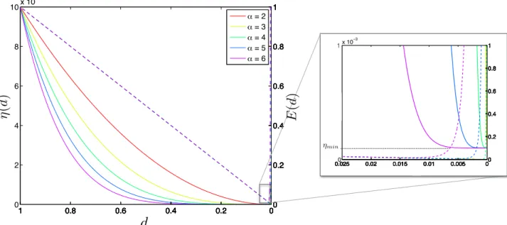
As introduced in section 2.1.2, the Maxwell-EB rheology di↵ers fundamentally from the standard Maxwell rheology in that the mechanical parameters E, ⌘ (and, as discussed below, ) are not constant but coupled to the spatially and temporally evolving level of damage of the simulated material, which controls its local degradation and re-increase in strength.

Consistent with previous damage rheological models, this property is represented in the Maxwell-EB frame-work by a dimensionless scalar parameter, d (e.g., Amitrano et al., 1999; Cowie et al., 1993; Tang, 1997; Hamiel et al., 2004, and others), and is interpreted as a measure of sub-grid cell defects or crack density (Kemeny and Cook, 1986). The value of d evolves between 1 (undamaged) and 0 (”completely damaged” material).

The level of damage is allowed to evolve through two competing mechanisms : damaging and healing. On the one hand, damaging represents fracturing and the opening of faults, or ”leads” in the case of sea ice, occurring when and where the internal stress exceeds the mechanical resistance of the material and which leads to its weakening. Healing on the other hand represents the reconsolidating and strengthening of the damaged material through sintering or, in the case of sea ice, refreezing within open leads. Although these mechanisms

also contribute to the increase in elastic sti↵ness (E _{⇥ h, with h, the ice thickness) and e↵ective apparent}

viscosity (⌘_{⇥ h) of the ice, healing is distinguished from pure thermodynamic growth or dynamically-driven}

thickness redistribution (e.g., Rothrock, 1975) in that it applies only where and when the material has been

damaged. It therefore allows d, E and ⌘ to re-increase at most to their undamaged value; d0_{= 1, E}0 _{and ⌘}0

respectively.

Because the two processes operate simultaneously within the simulated material, an evolution equation for d needs to include both mechanisms, while respecting the following constraints:

1. d decreases with damaging, which occurs only when the stress state becomes over-critical, 2. d increases with healing,

3. the increase in d due to healing cannot o↵set its decrease due to damaging, i.e., d cannot increase beyond its undamaged value of 1.

In the following, damaging and healing are first treated separately and then combined in a single equation for d.

Damaging

Contrary to typical sea ice modelling frameworks, no plastic (i.e., normal) flow rule is prescribed when the damage criterion is reached in the Maxwell-EB (and EB) model. Instead, when the stress locally exceeds the critical stress, the level of damage d and the elastic modulus, are allowed to drop, leading to local strain softening (Amitrano et al., 1999; Cowie et al., 1993; Tang, 1997). Because of the long-range interactions

within the elastic medium, local drops in E imply a stress redistribution that can in turn induce damaging of neighbouring elements (see figure 2.4). By this process, ”avalanches” of damaging events can occur and damage can propagate within the material over long distances (Amitrano et al., 1999; Girard et al., 2010a). As the elastic perturbation generated by such events is anisotropic (Eshelby, 1957), this propagation mechanism naturally leads to the emergence of both spatial heterogeneity and anisotropy in the stress and strain fields, i.e., to the formation of linear-like faults (see section 2.4).

d d d d d d d d d d d d d d d d d d d d t t + t _d t + 2 t d d d d d d d d d d d d d d d d d d d0 d d d d d d d d d d d d d d d d d0 d0 d0 d0

Figure 2.4: Schematic representation of the propagation of damage in the Maxwell-EB model. The domain is discretized in space using a (here, structured) mesh of triangular elements and the damage criterion is set through the field of cohesion C, in which noise is introduced at the scale of the element. Forcing, homogeneous or not, is applied on the simulated material as an external force or prescribed displacement and the internal stress within the simulated material builds up such that at time t it exceeds the damage criterion over a given element (circled in red). At the next time step, t + t, the element is by this fact weakened and its post-damaging level of damage is d0< d. Because it is weaker, the part of the internal stress it can no longer withstand is redistributed to its close neighbours through elastic interactions. By this redistribution, some of the neighbouring elements (circled in red) become in turn over-critical. At time t + 2 t, the weakening of these elements triggers further damaging events.

In the Maxwell-EB model, the change in level of damage corresponding to a local damage event is determined as a function of the distance of the damaged model element to the yield criterion. Three important assumptions

are made when calculating this distance, denoted in the following by dcrit. The first is that the deformation

of each model element is conserved during a damaging event, i.e., at initiation, damage modifies only the local state of stress, not strains. This assumption holds when considering not a single model element, but a matrix of elements. In this case, when damaging occurs locally and neighbouring elements remain undamaged, the first e↵ect is a stress redistribution between these neighbouring elements. The second assumption is that, for

a sufficiently small model time step t, i.e. very small compared to the viscous relaxation time (see section

2.2.4), a negligible part of the stress is dissipated into viscous deformations. A third constraint is based on the fact that stresses outside the failure envelope are not physical because brittle failure would occur before the material could support them. Hence we consider that damaging acts so that after being damaged, an element has its state of stress lying just on the failure envelope. With these assumptions made, the following equality holds for each damaged element:

"0= " _! K 1 0 E_{⇥ d}crit = K 1 E , (2.14)

where the superscript0_{denotes the post-damage state of deformation and stress (lying on the failure envelope).} Using Hooke’s law (given by 2.4 and here under plane stress conditions),

2 6 4 11 22 12 3 7 5 = E₁ 1_⌫2 2 6 4 1 ⌫ 0 ⌫ 1 0 0 0 1 ⌫₂ 3 7 5 2 6 4 "11 "22 2"12 3 7 5 ,