HAL Id: tel-02924854
https://tel.archives-ouvertes.fr/tel-02924854
Submitted on 28 Aug 2020HAL is a multi-disciplinary open access archive for the deposit and dissemination of sci-entific research documents, whether they are pub-lished or not. The documents may come from teaching and research institutions in France or abroad, or from public or private research centers.
L’archive ouverte pluridisciplinaire HAL, est destinée au dépôt et à la diffusion de documents scientifiques de niveau recherche, publiés ou non, émanant des établissements d’enseignement et de recherche français ou étrangers, des laboratoires publics ou privés.
constraint search
Pierre Talbot
To cite this version:
Pierre Talbot. Spacetime programming : a synchronous language for constraint search. Artificial Intelligence [cs.AI]. Sorbonne Université, 2018. English. �NNT : 2018SORUS416�. �tel-02924854�
SORBONNE UNIVERSITÉ Spécialité
Informatique
École doctorale Informatique, Télécommunications et Électronique (Paris) Présentée par
Pierre Talbot
Pour obtenir le grade de
DOCTEUR de SORBONNE UNIVERSITÉ
Sujet de la thèse :
Spacetime Programming
A Synchronous Language for Constraint Search
dirigée par Carlos Agon et encadrée par Philippe Esling soutenue le 6 juin 2018 devant le jury composé de :
M. Carlos Agon Directeur de thèse
Mme. Emmanuelle Encrenaz Examinatrice
M. Antoine Miné Examinateur
M. Vijay A. Saraswat Rapporteur
M. Manuel Serrano Examinateur
M. Sylvain Soliman Examinateur
M. Guido Tack Rapporteur
A Synchronous Language for Constraint Search
Pierre TalbotAbstract
Constraint programming is a paradigm for computing with mathematical rela-tions named constraints. It is a declarative approach to describe many real-world problems including scheduling, vehicles routing, biology and musical composition. Constraint programming must be contrasted with procedural approaches that de-scribe how a problem is solved, whereas constraint models dede-scribe what the prob-lem is. The part of how a constraint probprob-lem is solved is left to a general constraint solver. Unfortunately, there is no solving algorithm efficient enough to every prob-lem, because the search strategy must often be customized per problem to attain reasonable efficiency. This is a daunting task that requires expertise and good understanding on the solver’s intrinsics. Moreover, higher-level constraint-based languages provide limited support to specify search strategies.
In this dissertation, we tackle this challenge by designing a programming lan-guage for specifying search strategies. The dissertation is constructed around two axes: (i) a novel theory of constraint programming based on lattice theory, and (ii) a programming language, called spacetime programming, building on lattice theory for its data structures and on synchronous programming for its computa-tional model.
The first part formalizes the components of inference and search in a constraint solver. This allows us to scrutinize various constraint-based languages through the same underlying foundations. In this respect, we give the semantics of sev-eral paradigms including constraint logic programming and concurrent constraint programming using lattices. The second part is dedicated to building a practi-cal language where search strategies can be easily composed. Compositionality consists of taking several distinct strategies and, via some operators, to compose these in order to obtain a new strategy. Existing proposals include extensions to logic programming, monadic constraint programming and search combinators, but all suffer from different drawbacks as explained in the dissertation. The original aspect of spacetime programming is to make use of a temporal dimension, offered by the synchronous paradigm, to compose and synchronize search strategies on a shared logical clock.
This paradigm opens the door to new and more complex search strategies in constraint programming but also in applications requiring backtracking search. We demonstrated its usefulness in an interactive computer-aided composition sys-tem where we designed a search strategy to help the composer navigating in the state space generated by a musical constraint problem. We also explored a model checking algorithm where a model dynamically generates a constraint satisfaction problem (CSP) representing the reachability of some states. Although these ap-plications are experimental, they hint at the suitability of spacetime programming in a larger context.
Acknowledgements
Je remercie très chaleureusement Emmanuel Chailloux qui, après un Skype mémorable, m’a accepté pour ma dernière année en Master, et qui m’a trouvé un stage qui allait me diriger vers une thèse. Plutôt que de parler de stage, c’est plutôt vers Carlos, ou Carlito, après 4 ans on se le permet, et Philou, que j’ai été dirigé. Une histoire qui a commencé à “la salle de réunion”, et dans laquelle ils m’ont prodigué des conseils des plus avisés, et ce toujours dans une excellente ambiance.
Merci aussi à tous mes bro’ffices. Clément et Mattia avec qui tout ça a
commencé. Merci aux amis de Jussieu, et surtout l’équipe APR, Steven, Pierrick, Vincent, qui étaient là aux premières heures. Merci Rémy, tu m’as suivi sur les toutes les branches de la A, et puis même jusqu’à Châtelet (c’est ça la force de l’amitié). L’amicale de ping pong de l’IRCAM : merci à Gérard, Sylvie, Grégoire, Karim, Cyrielle, Florence, Olivier et tous les pongistes du −4. Et puis, merci Jean-Louis, Pierre N°2, et tous les autres.
I would like to acknowledge Vijay Saraswat, Guido Tack and Antoine Miné for their valuable comments and corrections on my dissertation.
I had the opportunity to go to Japan twice, and I am grateful for all the help Philippe Codognet provided me. Chiba-sensei and Phong Nguyen, warmly welcomed me to their labs in Japan, and I highly appreciate their support. Of course, special thanks to all of my friends in Japan: Marceau Suntory, Klervie, Nate, Mathieu Green Trompette, Nicolas and Guillaume. I would like to thank Thomas Silverston too, for the good time we spent together. Thanks to all these people, I had a very pleasant and inspiring stay in Tokyo.
I want to thank my wife, Yinghan, who continuously supports me, and always has faith in me.
Merci aussi à toute ma famille, ma mère, mon père, Céline et Thomas, pour m’avoir encouragé, et ce même parfois de l’autre bout du monde.
Pierre Talbot Paris, le 17 avril 2018
Contents
Introduction 1
I A Lattice Theory of Constraint Programming 9
1 Lattice Hierarchy for Constraint Solving 10
1.1 Constraint programming . . . 11
1.1.1 Constraint modelling . . . 11
1.1.2 Constraint solving . . . 13
1.1.3 Propagation . . . 16
1.2 Lattice structure . . . 18
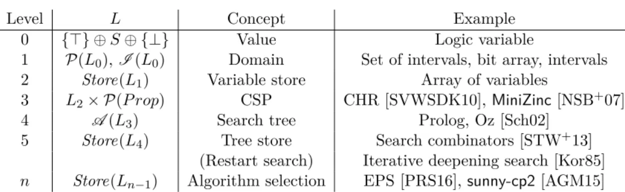
1.3 Lattice hierarchy for constraint programming . . . 27
1.3.1 L0: Value . . . 28
1.3.2 L1: Domain . . . 28
1.3.3 L2: Variable store . . . 29
1.3.4 L3: Constraint satisfaction problem . . . 29
1.3.5 L4: Search tree . . . 32
1.3.6 L5: Tree store . . . 33
1.3.7 Ln: Algorithm selection . . . 35
1.4 Inference in L3 with propagation . . . 35
1.4.1 Modelling a problem . . . 35
1.4.2 Deciding . . . 36
1.4.3 Propagating . . . 37
1.5 Bridging L3 and L4 with backtracking . . . 38
1.5.1 Delta operator . . . 40
1.5.2 Queueing strategy . . . 41
1.5.3 Branching strategy . . . 43
1.5.4 Exploration strategy . . . 45
1.6 Inference in L4 with constraint optimization problem . . . 46
1.7 Pruning in L4 with backjumping . . . 47
1.8 Conclusion and discussion . . . 50
2 Constraint-based Programming Languages 52 2.1 Introduction . . . 52 2.2 Background . . . 54 2.2.1 First-order logic . . . 55 2.2.2 Semi-decidability . . . 56 2.2.3 Logic programming . . . 57
2.2.4 Decidable fragments of FOL . . . 59
2.3 Modelling languages: from L0 to L4 (⊔) . . . 60
2.3.1 Declarative languages . . . 60
2.3.2 Constraint imperative programming . . . 65
2.4 Inference-based languages: from L0 to L3 (⊔, ⊨) . . . 67
2.4.1 Concurrent logic programming . . . 67
2.4.2 Concurrent constraint programming . . . 70
2.5 Bridging L3 and L4 (⊔, ⊨, ∆) . . . 78
2.5.1 Andorra-based languages . . . 78
2.5.2 Constraint logic programming . . . 81
2.5.3 Lattice-based semantics of CLP . . . 86
2.6 Search languages: L4 and above (⊔, ⊨, ∆) . . . 91
2.6.1 Search in logic languages . . . 92
2.6.2 Search in other paradigms . . . 97
2.6.3 Control operators for search . . . 101
2.7 Conclusion and discussion . . . 103
II Spacetime Programming 106 3 Overview of Spacetime Programming 107 3.1 Synchronous programming . . . 107
3.1.1 Linear time . . . 108
3.1.2 Causality analysis . . . 109
3.2 Concepts of spacetime programming . . . 111
3.2.1 Branching time . . . 111
3.2.2 Blending linear and branching time . . . 112
3.2.3 Host variables as lattice structures . . . 113
3.3 Syntax and intuitive semantics . . . 114
3.3.1 Communication fragment . . . 114
3.3.2 Undefinedness in three-valued logic . . . 117
3.3.3 Synchronous fragment . . . 118
3.3.4 Search tree fragment . . . 119
3.3.5 Read-write scheduling . . . 120
3.3.6 Derived statements . . . 121
3.4 Programming search strategies in L4 . . . 122
3.4.2 Branch and bound . . . 125
3.5 Hierarchy in spacetime with universes . . . 126
3.5.1 Universe fragment . . . 127
3.5.2 Communication across layers of the hierarchy . . . 128
3.6 Programming in L5 with universes . . . 130
3.6.1 Iterative deepening search . . . 130
3.6.2 Branch and bound revisited . . . 131
4 Behavioral Semantics Inside an Instant 134 4.1 Behavioral semantics . . . 134
4.2 Composition of search trees . . . 137
4.3 Expressions and interface with host . . . 139
4.4 Statements rules . . . 141
4.4.1 Communication fragment . . . 141
4.4.2 Synchronous fragment . . . 143
4.4.3 Search tree fragment . . . 145
4.5 Causality analysis . . . 146
4.5.1 Logical correctness . . . 146
4.5.2 A constraint model of causality . . . 147
4.5.3 From the spacetime program to the causality model . . . 150
4.5.4 Causal dependencies . . . 150
4.5.5 Causal statements . . . 152
4.6 Conclusion and discussion . . . 156
5 Behavioral Semantics Across Instants 159 5.1 Composition of parallel universes . . . 160
5.2 Universe hierarchy . . . 160
5.3 Hierarchical behavioral semantics . . . 163
5.4 Hierarchical variable . . . 164
5.4.1 Read, write and allocate variables in the hierarchy . . . 165
5.4.2 Top-down spacetime transfer . . . 167
5.4.3 Bottom-up spacetime transfer . . . 169
5.5 Semantics of the rules across time . . . 169
5.5.1 Semantics of the queueing strategy . . . 169
5.5.2 Universe statement . . . 171
5.5.3 Reaction rule . . . 172
III Applications 173 6 Modular Search Strategies 174 6.1 Pruning strategies . . . 174
6.1.1 Statistics . . . 174
6.2 Restart-based search strategies . . . 177
6.2.1 L5 search strategies . . . 177
6.2.2 Exhaustiveness and state space decomposition . . . 178
6.2.3 Composing L5 search strategies . . . 181
6.2.4 L6 search strategy . . . 183
6.3 Guarded commands . . . 184
7 Interactive Computer-Aided Composition 186 7.1 Introduction . . . 186
7.2 Score editor with constraints . . . 187
7.2.1 Visual constraint solving . . . 187
7.2.2 Spacetime for composition . . . 188
7.3 Interactive search strategies . . . 189
7.3.1 Stop and resume the search . . . 189
7.3.2 Lazy search tree . . . 190
7.3.3 Diagnostic of musical rules . . . 191
7.4 Conclusion . . . 192
8 Model Checking with Constraints 194 8.1 Model checking . . . 194
8.2 Model checking with constraints . . . 197
8.2.1 Constrained transition system . . . 197
8.2.2 Existential constraint system . . . 199
8.2.3 Lattice abstraction . . . 200
8.3 Spacetime algorithm . . . 202
8.4 Search strategies for verification . . . 204
8.4.1 Verifying constraint-based property . . . 204
8.4.2 Constraint entailment algorithm . . . 205
8.5 Conclusion . . . 207
IV Conclusion 208 9 Conclusion 209 10 Future work 211 10.1 Towards constraint programming with lattices . . . 211
10.2 Extensions of spacetime . . . 212
10.3 Beyond search in constraint programming . . . 215
Introduction
This dissertation links the paradigms of constraint programming and syn-chronous programming. We present these two fields in turn, and then we outline spacetime programming, the language proposed in this work for uni-fying these two paradigms.
Constraint programming
In theoretical computer science, a function models a correspondence between the sets of input and output states, while a relation expresses a property that must be satisfied by the computation. Operationally, functions and relations are em-bodied in deterministic and non-deterministic computations. From an expressive standpoint, this distinction is artificial since any algorithm described by a non-deterministic algorithm can be described by a non-deterministic equivalent one.1 So
what is the advantage of using one model of computation over the other? The answer is that sometimes it is much easier to express what properties a solution must satisfy than to specify how we should compute this solution. This dual view is at the heart of the differences between imperative and declarative program-ming paradigms, which allow us to program respectively the how and the what. Around 1970, logic programming emerged as a paradigm conciliating these two views, where a declarative program also has an executable semantics [Kow74]. In this dissertation, we focus on a generalization of the logic computational model called constraint programming.
Constraint programming is a paradigm for expressing problems in terms of mathematical relations—called constraints—over variables (e.g. x > y). Con-straints are an intuitive approach to naturally describe many real-world problems which initially emerged as a subfield of artificial intelligence and operational re-search. The flagship applications in constraint programming encompass schedul-ing, configuration and vehicles routing problems; all of these three have a chapter in [RvBW06]. Constraints are also applied to various other domains such as in music [TA11, TAE17], biology [RvBW06] and model checking [CRVH08, TP17]. Besides its application in practical fields, constraint programming is also the theory of efficient algorithms for solving constraint satisfaction problems (CSP).
1
However, the complexity of these two algorithms might not be equivalent; answering this question is the famous P̸=NP problem.
In this dissertation we are interested in how a CSP is solved. Constraint solving usually relies on a backtracking algorithm enumerating the values of the variables until a solution is found, i.e. all the constraints are satisfied. This algorithm gen-erates a search tree where every branch reflects a choice made on one variable. In case of unsatisfiability, the algorithm backtracks in the search tree to the previous choice and try another branch. For example, consider the CSP with two variables x and y both taking a value in the set {1, 2} (called the domain of the variable), and the constraint x ̸= y. We first assign x to 1, and then y to 1 which result in an unsatisfiable CSP because x ̸= y does not hold. Therefore, we backtrack in the search tree by trying another branch which assigns y to 2. This time we obtain a solution where x = 1 and y = 2. The algorithm exploring the search tree is called a search strategy.
Synchronous programming
The synchronous paradigm [Hal92] proposes a notion of logical time dividing the execution of a program into a sequence of discrete instants. The main goal of log-ical time is to coordinate processes that are executed concurrently while avoiding typical issues of parallelism, such as deadlock or indeterminism [Lee06]. During one instant, processes execute a statically bounded number of actions—unbounded loop or recursion are prohibited—and wait for each other before the next instant. Although the programmer views a synchronous program as a set of processes evolving more or less independently, the processes are scheduled sequentially at runtime. In other words, every instruction of each process happens before or after another one. An important aspect of the synchronous model is that a causality analysis ensures programs to be deterministic (resp. reactive): at most (resp. at least) one output is produced from one input. It implies that even if the program can be sequentialized in different ways, it will always produce a unique result.
Concretely, we can implement a synchronous program as a coroutine: a function that maintains its state between two calls. A call to the coroutine triggers the ex-ecution of one instant. We must precise that the coroutine is generally called from a host language interfacing between the user environment and the synchronous program.
In this dissertation, we focus on the imperative synchronous language Es-terel [Ber00b]. The input and output data of an EsEs-terel program are boolean variables called signals. A simple example of an Esterel program is a watch: its state changes when the user presses buttons or when a second has elapsed. We can imagine the buttons of the watch being boolean variables, and every process implements the logic of one button. The causality analysis warns the programmer about corner cases that he forgot to implement. For example, if the user presses two buttons at the same time, and that their processes produce two output states that are conflictual.
Motivation
On the language side of constraint programming, pioneered by logic programming, an influential paper of Kowalski captures the how and the what in the equation “Algorithm = Logic + Control” [Kow79]. In the early day of logic programming, a hope was to keep the control aspect hidden from the programmer who would only specify the logic part of its program. Forty years have passed by but a solving algorithm that is efficient for every problem is yet to be found. We quote Ehud Shapiro [Sha86] who already commented on this illusory hope back in 1986:
The search for the ultimate control facility is just the search for the “philosopher’s” stone in disguise. It is similar to the search for the gen-eral problem-solver, or for the gengen-eral efficient theorem-prover, which simply does not exist. We have strong evidence today that many classes of seemingly simple problems have no general efficient solution.
The logic part has been extensively studied with constraint modelling lan-guages [Lau78, VHMPR99, NSB+07] and it is well-understood today. However,
while these languages are outstanding for the logic specification of combinatorial problems (often NP-complete), the specification alone generally leads to poor per-formances. This is why some limited form of controls exist in Prolog, such as the controversial cut operator that prunes the search tree. Numerous approaches have been designed to provide language abstractions for specifying the control part of constraint solving [VH89, LC98, VHML05]. A fundamental question in these approaches is the compositionality of search strategies: how can we easily com-bine two strategies and form a third? Recently, we witness a growing number of proposals [SSW09, STW+13, MFS15] that attempt to cope with this
composition-ality issue. This problematic is central in the design of the spacetime programming language developed over this dissertation.
A search language is important because experience has proven that reducing the solving time of combinatorial problems, especially in industry, must be tackled per problem or even per problem-instance after the design and test of several solver configurations and search strategies [SO08, TFF12]. Therefore, we need to easily try and test the efficiency of new search strategies for a given problem. Currently, the implementers of search strategies have to choose between limited but high-level specification languages and full-fledged but low-level constraint libraries. The first family encompasses constraint logic programming where control is obtained with predetermined building blocks assembled within a search predicate. For example, GNU-Prolog [DAC12] proposes the predicate fd_labelling/2 where the first argu-ment is the list of variables and the second some options for selecting the variables and values enumeration strategies. The second family concerns constraint libraries such as Choco [PFL15] or GeCode [STL14] which are designed to be extensible and opened to search programming while remaining very efficient. The main problem of the library approach is that users need good understanding of the intrinsics of
the library but only experts are knowledgeable in this domain. Of course, many works attempt to bridge the gap between these two extreme categories, which we will discuss in Chapter 2.
Overview
In Part I, we contribute to a theoretical framework of CSPs based on lattice theory. Part II formalizes the syntax and semantics of spacetime programming based on the lattice framework developed in the first part. Finally, in Part III, we develop three applications of search strategies written in the spacetime paradigm. These applications develop on the interactive and hierarchical aspects of spacetime pro-gramming. We outline the content of each part in the following paragraphs. Part I: A lattice theory of constraint programming
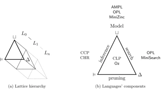
In Chapter 1, we formulate a lattice theory of constraint programming for finite
domains where constraint inference is based on the denotational model introduced
in [Tac09]. As far as we know, our theory is the first attempt to formalize the structures underlying the inference and search components in a unified framework. The main idea is to define a hierarchy of lattices where each level is built on the powerset of the previous level. This hierarchical structure is central to constraint programming, as the notions of domain, constraint and search tree depend on each other. In Chapter 2, we review a large spectrum of constraint-based programming languages. A new aspect of this study is to classify the various languages within the hierarchy levels developed in the former chapter. To demonstrate the gener-ality of our lattice hierarchy, we develop the lattice-based semantics of concurrent constraint programming [Sar93] and constraint logic programming [MJMS98]. We pinpoint several issues in modern search languages that are tackled by spacetime programming later in our proposal.
Part II: Spacetime programming
In order to tackle the compositionality issue, our approach is to link constraint pro-gramming and synchronous propro-gramming in a unified language, called spacetime
programming or “spacetime” for short. We briefly explain its model of
computa-tion and how its construccomputa-tions are relevant to the lattice hierarchy developed in Chapter 1.
Computational model Spacetime inherits most of the temporal statements of
Esterel, including the delay, parallel, loop, suspension and abortion statements. We connect the search tree induced by constraint programming and the linear time of synchronous programming with a principle summarized as follows:
Our key observation is that search strategies are synchronous processes exploring a search tree at a same pace. A challenge is introduced by the notion of linear time exploring a tree-shaped space: how does the variables evolve in time and space in a coherent way? We propose to annotate variables with a spacetime attribute to distinguish between variables local to one instant (single_time), variables global to the whole computation (single_space) and backtrackable variables local to a branch in the search tree (world_line). For example, a global variable can be used to count the number of nodes in the search tree, and a backtrackable variable can be the constraint problem itself.
Variables defined on lattices The second characteristic of spacetime is inherited
from concurrent constraint programming (CCP) [Sar93] where the memory is de-fined by a global constraint store accumulating partial information. Processes can communicate and synchronize through this store with two primitives: tell(c) for adding a constraint c into the store and ask(c) for asking if c can be deduced from the store. Concurrency is treated by requiring the store to grow monotonically, i.e. removal of information is not permitted. The difference of spacetime with CCP is that variables are all defined over lattice structures, instead of having a central and global constraint store. The tell and ask operations in spacetime are defined on lattices, where tell relies on the least upper bound operation and ask relies on the order of the lattice. These lattice operations effectively relate the framework developed in Chapter 1 and the spacetime language. Besides, we must note that the lattice structures are programmed in the host language of spacetime. This al-lows the user of spacetime to reuse existing constraint solvers which are abstracted as lattice variables.
Causality analysis From a synchronous perspective, every instant of a spacetime
process is a monotonic function over its lattice variables. This property is ensured by the causality analysis of spacetime (Section 4.5). It is an important contribution because current synchronous languages are defined on a restricted class of lattices, called flat lattices. We refine the behavioral semantics of Esterel [Ber02] to lattice-based variables which imply scheduling read and write operations correctly. A correct scheduling is crucial to preserve the deterministic and reactive properties of a synchronous program.
Hierarchical computation The fourth concept synthesizes time hierarchy from
synchronous programming and spatial hierarchy from logic programming. Time hierarchies were first developed in Quartz [GBS13] and ReactiveML [Pas13, MPP15] to execute a process on a faster time scale. They propose that in one instant of the global clock, we can execute more than one local step of a process. Spatial hierarchies were introduced with logic programming and more particularly with deep guards and computation spaces in the Oz programming language [Sch02]. It executes a process locally with its own queue of nodes.
We propose the concept of universe which encapsulates the spatial and time dimensions of a computation. Basically a universe extends a computation space to a clock controlling the evolution of its variables through time. In the lattice hierarchy, a universe enables users to create an additional layer in the hierarchy. This extension is particularly useful to write search strategies that restart the search or explore several times a search tree. For example, by encapsulating a process in a universe exploring a search tree, we can manipulate a collection of search trees, where in each instant we explore a new search tree. The concept of universe essentially implements the powerset derivation defining the levels of the lattice hierarchy.
Part III: Applications
This last part studies three applications of spacetime programming built on search strategies developed in the spacetime paradigm. In Chapter 6, we show how to design a modular library of search strategies. It also illustrates that spacetime is applicable to specialized and complex search strategies in the field of constraint programming. Beyond constraint programming, spacetime is also suited to im-plement interactive applications. In particular, we introduce in Chapter 7 an interactive search strategy for a computer-aided composition system allowing the composer to dynamically navigate in the state space generated by a musical CSP. It attempts to put back constraints at the heart of the compositional process in-stead of solving musical problems in a black box fashion. Finally, we expand the scope of spacetime programming to model checking where we explore a new al-gorithm based on a constraint store to solve parametric model checking problems (Chapter 8).
Summary
To summarize, we introduce a programming language, called spacetime
program-ming, to control the evolution of lattice structures through a notion of logical
time. To demonstrate the capabilities of our proposal, we study CSPs as lattice structures, which is a general framework for specifying and solving combinatorial problems. A long-standing issue in this field, started with logic programming in the seventies, is how to compose two existing search strategies. We demonstrate that logical time is an excellent abstraction to program and combine search strategies in order to solve a combinatorial problem. We extend the scope of this paradigm by investigating an interactive computer-aided composition software and a model checking algorithm based on constraints.
Contributions
• A hierarchical lattice theory unifying the modelling and search compo-nents (i.e. what and how) of constraint programming (Chapter 1).
• A survey of constraint-based programming languages that classifies and formalizes constraint languages according to the lattice hierarchy (Chap-ter 2). The main insight is that many constraint-based languages can be defined over the same structure, which helps in better understanding their differences.
• The semantics of spacetime programming provides the foundations for com-posing search strategies which are synchronous processes over the lattice hierarchy (Chapters 3, 4 and 5). The originality is to map logical time to the exploration of the search tree.
• We propose a causality analysis of a spacetime program for variables defined over lattices. It extends the causality analysis of Esterel which is defined for boolean variables only.
• We show that modular, interactive and hierarchical search strategies can be programmed in the spacetime language (Chapters 6, 7, and 8). How to read this document
This dissertation is organized in 10 chapters that can be read in different ways. We show the dependencies between the different chapters or parts in Figure 1. For a short tour of the dissertation, we suggest to read Section 1.3 for the lattice foundation, Chapter 3 for the overview of spacetime, and Chapter 7 for a more in-depth example of an interactive search strategy for musical composition. The survey in Chapter 2 can be read apart from the spacetime language.
Chap. 1 Lattice for constraint solving (Section 1.3)
Chap. 2 Survey Chap. 3 Overview of spacetime
Chap. 4,5 Semantics of spacetime
Part III Applications Part IV Conclusion Figure 1: Organization of the dissertation.
Part I
A Lattice Theory of Constraint
Programming
Lattice Hierarchy for Constraint Solving
Over the years, numerous techniques have been devised to solve constraint problems and to improve the efficiency of existing algorithms. They range from low-level considerations such as memory management to higher-level techniques, such as propagating constraint, learning new constraints, and intelligently split-ting a state space. The current foundation of constraint programming is built on a set theoretic definition of the constraint problem, which is explained in Sec-tion 1.1. However, solving techniques frequently use more complex combinatorial objects rather than the constraint problem structure alone. A prime example of such objects is the search tree—a structure to enumerate all the solutions, which is implicitly generated by the solving algorithm only. Since every algorithm is different, we do not have a common ground to understand the subtle differences among these techniques in terms of how they cooperate and integrate with each other. Therefore, in order to understand the relations among available techniques, we believe that a more extensive foundation of constraint programming is needed. The purpose of this chapter is to devise a new foundation for constraint pro-gramming, in which all the combinatorial structures are explicitly defined. To achieve this, we rely on the theory of lattices to precisely capture the combinato-rial objects underlying constraint solving. To make this chapter self-contained, we introduce the basics of lattice theory in Section 1.2. Next, we organise the combi-natorial objects of constraint programming in a hierarchy where each level relies on the levels before it (Section 1.3). For example, relations are defined onto variables; a search tree is a collection of partially solved constraint problems. Once this structure defined, we present several key constraint solving techniques as mono-tonic functions over this hierarchy. Furthermore, with an algebraic view of lattices, we demonstrate that most algorithms are defined by a combination of three lattice operators. This finding provides a common ground for many techniques including constraint propagation (Section 1.4), backtracking search (Section 1.5), optimiza-tion problems (Secoptimiza-tion 1.6) and backjumping (Secoptimiza-tion 1.7). Of course, as discussed in Section 1.8, there are more techniques that are interesting to study through the lattice theory. We limit the scope of this chapter to exhaustive solving algorithms
over finite domains, and thus finite lattices, which is one of the most successful settings of constraint programming.
1.1
Constraint programming
Constraint programming is a declarative paradigm for solving constraint satis-faction problems (CSPs) [RvBW06]. The programmers only need to declare the structure of a problem with constraints (e.g. x > y ∧ x ̸= z) and it is auto-matically solved for them. We illustrate the modelling aspect of constraint pro-gramming in Section 1.1.1 with a musical problem. Under the hood, constraint solving usually relies on a backtracking algorithm enumerating the values of the variables until we find a solution, i.e. all the constraints are satisfied. We in-troduce a mathematical framework for solving finite CSPs in Section 1.1.2 which is based on the dissertation of Guido Tack [Tac09]. In contrast, other heuris-tic methods such as local search, not guaranteeing to find a solution, are left out of scope in this dissertation. What’s more, in Section 1.1.3, we focus on a propagation-based algorithm which is a technique used in almost every constraint solver (e.g. [STL14, PFL15, GJM06, IBM15]). The lattice framework developed in the rest of this chapter is built on the definitions introduced here.
1.1.1 Constraint modelling
As a first example of constraint modelling problem, we consider the all interval-series (AIS) musical problem1
, for example described in [MS74]. It constrains the pitches of the notes as well as the intervals between two successive pitches to be all different. Initially, the pitches are initialized in the interval domain [1..12]. The domains are pictured by the rectangles on the following score:
& 124
Throughout the solving process, the domains become smaller, and are eventually instantiated to a note when we reach a solution. An example of such a solution is:
& 124
#
n
n
n
#
n
n
n
n
#
n
# n# n n
n
For the composer, it forms a raw material that can be transformed again using others tools such as OpenMusic [AADR98].
The AIS problem can be specified using a constraint modelling language. We illustrate this using MiniZinc [NSB+07] which is one of the most popular modelling
languages.
1
int: n = 12;
array[1..n] of var 1..n: pitches; array[1..n-1] of var 1..n-1: intervals; constraint forall(i in 1..n-1)
(intervals[i] = abs(pitches[i+1] - pitches[i]));
constraint forall(i,j in 1..n where i != j)
(pitches[i] != pitches[j]);
constraint forall(i,j in 1..n-1 where i != j)
(intervals[i] != intervals[j]);
solve satisfy;
This code is purely declarative. The arrays pitches and intervals are respec-tively storing the pitches and the differences between these pitches. The macro forall(r)(c)generates—at compile time—a conjunction of the constraints ci for
each i in the range expression r. The first forall is used to initialize the array intervalswith the absolute difference between two pitches. Due to the relational semantics of constraints, the equality predicate = ensures that the value of an interval is synchronized with every pair of successive pitches. Hence, we can read the equality in both directions: the pitches constrain the interval and the interval also constrains the pitches. The last two forall statements generate inequality constraints ensuring that all pitches and intervals are pairwise distinct. It remains the statement solve satisfy which is a “solve button” for obtaining a solution to this model from the system.
One of the principal reason behind the efficiency of a constraint solver is the presence of global constraints. A global constraint is a n-ary relation captur-ing a structure that abstracts a common modellcaptur-ing sub-problem. For example, the global constraint alldifferent({x1, . . . , xn}) enforces that the set of
vari-ables {x1, . . . , xn}contains only different values. A catalogue of the most common
global constraints has been established [BCR11] and is updated continuously to incorporate the newest constraints. A large body of work in the constraint pro-gramming community is the design of efficient algorithms for existing and novel global constraints but it is out of scope in this work. Back to the AIS example, we observe that the last two forall generators are actually both enforcing the alldifferentglobal constraints on different arrays. In MiniZinc, we can improve the model with the alldifferent global constraints provided by the system:
(...)
constraint alldifferent(pitches); constraint alldifferent(intervals); solve satisfy;
Actually, we initially provided a decomposition of the alldifferent constraint into a conjunction of more elementary constraints. It means that any solver supporting these elementary constraints also supports this global constraint. However, in practice, global constraints are usually mapped to more efficient but lower-level algorithms.
The interested reader can find more information and references about constraint modelling in [RvBW06].
1.1.2 Constraint solving
In this thesis, we will be mostly concerned with the constraint solving algorithms behind the “solve button”. We start by giving the mathematical foundations for constraint solving and several examples. These definitions are based on [Tac09]. Definition 1.1 (Assignment function). Given a finite set of variables X and a finite set of values V , an assignment function a : X → V maps every variable to a value. We note the set of all assignments Asndef= VX where VX is the set of all
functions from X to V .
In addition, we define a partial assignment which is an assignment such that at least one variable is mapped to more than one value.
Given a set S, we use P(S) to denote the powerset of S.
Definition 1.2 (Constraint satisfaction problem (CSP)). A CSP is a tuple ⟨d, C⟩ where
• The domain function d : X → P (V ) maps every variable to a set of values called the domain of the variable.
• The constraint set C is a subset of the powerset P (Asn).
An alternative but equivalent presentation of a CSP is the tuple ⟨X, D, C⟩ where the set of variables X and of domains D are made distinct while, in our case, it is embedded in the domain function d. In our framework, a constraint c ∈ C is defined in extension since c is the set of all assignments satisfied by this constraint. Thus, any assignment a ∈ c is a solution of the constraint c. For example, the constraint x < y is induced by the set {a ∈ Asn | a(x) < a(y)}.
The domain function itself can be viewed as a constraint con(d) defined by its set of assignments, and an assignment a ∈ Asn as a domain function:
con(d)def= {a ∈ Asn | ∀x ∈ X, a(x) ∈ d(x)} dom(a)def= ∀x ∈ X, d(x) 7→ {a(x)}
From these definitions, we can define the set of solutions of a CSP ⟨d, C⟩ as sol(⟨d, C⟩)def= {a ∈ con(d) | ∀c ∈ C, a ∈ c}
This mathematical framework leads to a “generate-and-test” backtracking al-gorithm. It enumerates all the possible combinations of values in the variables’ domains and tests for each assignment if the constraint set is satisfied. Modern constraint solvers offer many optimizations building on this backtracking algo-rithm. To start with, we consider the “propagate-and-search” algorithm which interleaves two key steps:
Algorithm 1 Propagate-and-search solve(⟨d, C⟩) Input: A CSP ⟨d, C⟩
Output: The set of all the solutions
1: d′ ← propagate(⟨d, C⟩)
2: if d′= ∅ then
3: return ∅
4: else if d′ = {a} then
5: return {a} 6: else 7: ⟨d1, . . . , dn⟩ ← branch(d′) 8: return ∪n i=0solve(⟨di, C⟩) 9: end if
1. Propagation as an inference mechanism for removing values from the vari-ables’ domains that do not satisfy at least one constraint.
2. Search successively enumerates the different values in the variables’ domains. The domains are backtracked to another choice if the former did not lead to a solution.
We define more precisely these two components and then give the full algorithm. We see propagation abstractly as a function propagate(⟨d, C⟩) 7→ d′ mapping a
CSP ⟨d, C⟩ to a reduced domain d′ which is empty if the problem is unsatisfiable.
We spend some times explaining propagation in more depth thereafter, but we give a first example of the propagation mechanism.
Example 1.1 (Propagation of x > y). Consider the following CSP ⟨{x 7→ {0, 1, 2}, y 7→ {0, 1, 2}}, {x > y}⟩
where x and y take values in the set {0, 1, 2} and are subject to the constraint x > y. Without enumerating any value, we can already remove 0 from the domain of x and 2 from the domain of y since there is no solution with such partial assignment. Applying propagate to this problem maps to the domain function:
{x 7→ {1, 2}, y 7→ {0, 1}}
⌟ The second component, search, relies on a branching function splitting the domain into several complementary sub-domains.
Definition 1.3 (Branching function). The function branch(d) 7→ (d1, . . . , dn)
maps a domain function d to a sequence of domain functions (d1, . . . , dn) such
that:
(i) con(d) =∪
i∈[1..n]con(di) (complete)
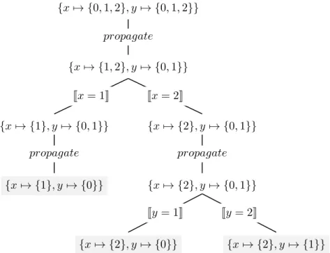
The two conditions ensure that splitting a domain must not remove some po-tential solutions (completeness) and must strictly reduce the domain set (strict monotonicity). This last condition is necessary to ensure the termination of the enumeration algorithm. {x 7→ {0, 1, 2}, y 7→ {0, 1, 2}} {x 7→ {1, 2}, y 7→ {0, 1}} {x 7→ {1}, y 7→ {0, 1}} {x 7→ {1}, y 7→ {0}} {x 7→ {2}, y 7→ {0, 1}} {x 7→ {2}, y 7→ {0, 1}} {x 7→ {2}, y 7→ {0}} {x 7→ {2}, y 7→ {1}} propagate Jx = 1K Jx = 2K propagate propagate Jy = 1K Jy = 2K
Figure 1.1: Search tree generated by the propagate-and-search algorithm.
Propagation and search are assembled in a backtracking algorithm presented in Algorithm 1. Whenever we obtain an empty domain d′, we return an empty
solution’s set indicating that the input CSP has no solution. If the domain d′ is
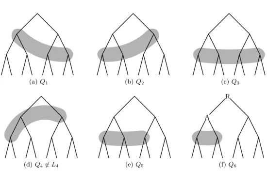
an assignment after propagation, it ensures that it is a solution and we return it. The successive interleaving of choices and backtracks leads to the construction of a search tree. All in all, a search tree is obtained by recursively applying the branching function on the CSP, and by propagating the domains in each node. Example 1.2 (Search tree of x > y). In Figure 1.1, we unroll the propagate-and-search algorithm on the CSP given in the Example 1.1. It alternates between propagation and branching until we reach a leaf of the search tree which are all solutions (highlighted in grey). In this case, the branching function is a flat enu-meration of the values in the domains, we will see other branching strategies in
Section 1.5.3. ⌟
Constraint optimization problems
One of the most important variations of the propagate-and-search algorithm is for solving constraint optimization problems. Instead of finding one or all solutions, we
want to find the best solution according to an objective function. More specifically, given an objective function f(x) where x is a variable, it tries to find a solution in which the value of x minimizes or maximizes f(x). The usual algorithm is branch
and bound: every time we reach a solution, we constrain the CSP such that the
next solution is forced to be better (in the sense of the objective function). In branch and bound, the objective function is implemented with a constraint that is added globally to the CSP during the search. We delay the explanation of a more formal definition to Section 1.6.
1.1.3 Propagation
In the former definitions, constraints are given in an extensive manner but this is poorly suited for implementation purposes. To improve efficiency, we rely on the notion of propagator, which is a function representing a constraint. The role of a propagator is twofold: pruning the domain and deciding if an assignment is valid with regard to its induced constraint.
Definition 1.4 (Propagator). Let Dom def
= P(V )X be the set of all the possible
domain functions. Given a function p : Dom → Dom, we say that a ∈ Asn is a solution of p if p(dom(a)) = dom(a). Then, p is a propagator if it satisfies the following properties:
(P 1) ∀d ∈ Dom, p(d) ⊆ d (contracting)
(P 2) For any solution a of p and ∀d ∈ Dom, (sound)
dom(a) ⊆ d implies dom(a) ⊆ p(d)
where the inclusion between two domain functions d ⊆ d′ is defined if ∀x ∈ X, d(x) ⊆
d′(x).
The contracting property ensures that a propagator p can only reduce domains and the soundness ensures that p cannot reject valid assignments. A constraint cp ∈ C
is induced by a propagator p ∈ P rop if cp = {a ∈ Asn | p(dom(a)) = dom(a)}, i.e.
the set of all solutions of p, where P rop is the set of all propagators. Therefore, for a single constraint, there are several propagators that are more or less contracting but implement the same constraint. In the following, we use the function JcK to denote a propagator function for a constraint c, e.g. Jx > yK. We stay abstract over the exact definition of a propagator. The fact that it induces its constraint is generally enough.
Definition 1.5 (Propagation problem). A propagation problem ⟨d, P ⟩ where d is the domain function and P ⊆ P rop is the set of propagators is equivalent to the CSP:
⟨d, {cp ∈ C | p ∈ P }⟩
The propagate-and-search algorithm can be directly adapted to deal with a prop-agation problem.
Intuitively, the function propagate(⟨d, P ⟩) reduces the domain d by computing a fixed point of p1(p2(. . . pn(d))) for every pi ∈ P. Reaching a fixed point indicates
that the propagators cannot infer additional information anymore and that we need to branch for progressing. This fixed point computation can be adequately formalized by viewing propagation as a transition system [Tac09].
Definition 1.6 (Transition system). A transition system is a pair ⟨S, →⟩ where S is the set of states and → the set of transitions between these states.
Definition 1.7 (Propagation-based transition system). The transition system of a propagation problem is a pair ⟨Dom, →⟩ where the transition →: Dom × P rop ×
Dom models the application of a propagator to the domain. We require that any
transition (d, p, d′) ∈→, noted d−→ dp ′, satisfies the following properties:
(P 1) p(d) = d′ (propagating)
(P 2) dom(p(d)) ⊂ dom(d) (strictly monotonic)
The transition is lifted to CSP structures ⟨d, P ⟩ −→ ⟨dp ′, P ⟩ with the additional
condition that p ∈ P . We write its transitive closure as ⟨d, P ⟩ ⇒ ⟨d′, P ⟩ where
⟨d′, P ⟩ is necessarily a fixed point of the transition system.
It forms a non-deterministic transition system: there are more than one possible transition that can be applied on some states. Hence, there exists various algo-rithms for deciding in which order to apply the transitions in order to reach a fixed point faster. For example, we refer to [Tac09, PLDJ14] for more information on the various propagation algorithms. The following abstract definition of propagation will be sufficient in this dissertation.
Definition 1.8 (Propagation). Let ⟨d, P ⟩ be a propagation problem, the propagation function is defined as
propagate(⟨d, P ⟩) 7→ ⟨d′, P ⟩ where ⟨d, P ⟩ ⇒ ⟨d′, P ⟩
Lastly, we give an important property of the propagation-based transition sys-tem.
Theorem 1.1 (Confluence). The fixed point of the transition system is unique if all the propagators are contracting, sound and monotonic (i.e. d ⊆ d′ ⇒ p(d) ⊆
p(d′)). Hence, the transition system is confluent.
1.2
Lattice structure
We first recall some definitions on complete lattices and introduce some notations2.
Definition 1.9 (Orders). An ordered set is a pair ⟨P, ≤⟩ where P is a set equipped with a binary relation ≤, called the order of P , such that for all x, y, z ∈ P , ≤ satisfies the following properties:
(P 1) x ≤ x (reflexivity)
(P 2) x ≤ y ∧ y ≤ x =⇒ x = y (antisymmetry)
(P 3) x ≤ y ∧ y ≤ z =⇒ x ≤ z (transitivity)
(P 4) x ≤ y ∨ y ≤ x (linearity)
An order is partial if the relation ≤ only satisfies the properties P1-P3, that is, it is not defined for every pair of elements. In this case, we refer to the set P as a partially ordered set (poset). Otherwise, the order is total and the set is said to be totally ordered.
In case of ambiguity, we refer to the ordering of the set P as ≤P and similarly
for any operation defined on P . We can classify functions with several properties when applied to ordered sets.
Definition 1.10. Given the ordered sets P and Q, and x, y ∈ P , a function f : P → Q is said to be order-preserving (or monotonic) if x ≤P y ⇒ f (x) ≤Q
f (y), an embedding if in addition the function is injective and an
order-isomorphism if the function is bijective.
We will focus on a particular class of ordered structures, namely lattices, and we introduce several definitions beforehand.
Definition 1.11 (Upper and lower bounds). Let ⟨L, ≤⟩ be an ordered set and S ⊆ L. Then
• x ∈ L is a lower bound of S if ∀y ∈ S, x ≤ y,
• Sℓ denotes the set of all the lower bounds of S,
• x ∈ L is the greatest lower bound of S if ∀y ∈ Sℓ, x ≥ y.
The (least) upper bound and the set of all upper bounds Su are defined dually by
reversing the order (using ≥ instead of ≤ in the definitions and vice-versa). Definition 1.12 (Lattice). An ordered set ⟨L, ≤⟩ is a lattice if every pair of ele-ments x, y ∈ L has both a least upper bound and a greatest lower bound.
2
Definition 1.13 (Complete lattice). A lattice ⟨L, ≤⟩ is complete if every subset of S ⊆ L has both a least upper bound and a greatest lower bound. A complete lattice is always bounded: there is a supremum ⊤ ∈ L such that ∀x ∈ L, x ≤ ⊤ and an infimum ⊥ ∈ L such that ∀x ∈ L, ⊥ ≤ x.
As a matter of convenience and when no ambiguity arises, we simply write L instead of ⟨L, ≤⟩ when referring to ordered structures. An alternative presentation is to view a lattice as an algebraic structure.
Definition 1.14 (Lattice as algebraic structure). A lattice is an algebraic structure ⟨L, ⊔, ⊓⟩ where the binary operation ⊔ is called the join and ⊓ the meet. The join x ⊔ y is the least upper bound of the set {x, y} and the meet x ⊓ y is its greatest
lower bound. We use the notation ⊔ S (resp. dS) to compute the least upper
bound (resp. greatest lower bound) of the set S.
As shown in [DP02], the operations ⊔ and ⊓ satisfy several algebraic laws. Theorem 1.2. Let L be a lattice and x, y, z ∈ L. Then
(L1) x ⊔ (y ⊔ z) ≡ (x ⊔ y) ⊔ z (associative law)
(L2) x ⊔ y ≡ y ⊔ x (commutative law)
(L3) x ⊔ x ≡ x (idempotent law)
(L4) x ⊔ (x ⊓ y) ≡ x (absorption law)
We obtain the dual laws by exchanging ⊔ with ⊓ and vice-versa.
The distinction between lattices and complete lattices only arises for infinite sets since any finite lattice is complete [DP02]. The proof of this claim is given by unfolding an expression ⊔ S as an expression ∀si ∈ S, s1⊔ . . . ⊔ sn, by application
of the associativity law 1.2(L1), we obtain a unique element. In the following, we consider lattices to be finite as it is usually the case in the field of constraint pro-gramming. Extending the framework developed in this chapter to infinite lattices is of great interest but is left to future works.
To complete this short introduction, we define the notion of sublattice which is a subset of a lattice that is itself a lattice.
Definition 1.15 (Sublattice). Let ⟨L, ≤⟩ be a lattice and S ⊆ L. Then S is a sublattice of L if for each x, y ∈ S we have x ⊔Ly ∈ S and x ⊓Ly ∈ S.
In the following, we interpret the order of a lattice ≤ in the sense of information systems. It views the element bottom ⊥ as being the element with the fewer information and the element top ⊤ as the element that contains all the information. This “contains more information than” order is noted |= and named the entailment operator. The entailment relation is often the inverse of the intuitive order of a lattice. This has no impact on the mathematical ground since, by the duality principle, any theorem on a (complete) lattice is also valid for its inverse order. Note that our usage of the symbol |= is not directly relevant to logical consequence and should be understood only as an order symbol.
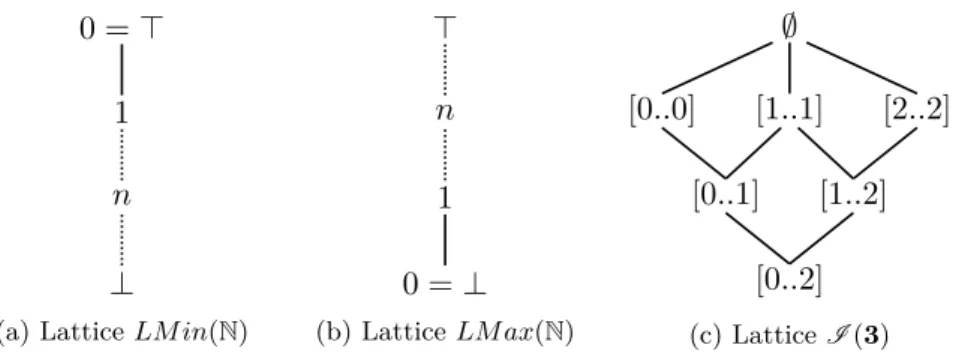
0 = ⊤ 1 n ⊥
(a) Lattice LM in(N)
⊤ n 1 0 = ⊥ (b) Lattice LM ax(N) [0..2] [0..1] [1..2] [0..0] [1..1] [2..2] ∅ (c) Lattice I (3)
Figure 1.2: Examples of lattices’ diagrams.
Notation 1.1 (Defining new lattice). We define a new lattice as L = ⟨S, |=⟩ where S is its set of elements and |= the order. Sometimes, the set S is already a lattice by construction, for example the Cartesian product of two lattices is a lattice. In this case, we omit the order which is inherited from S and we write L = S. When necessary, because we often manipulate lattices defined over other lattices, we disambiguate the order of a lattice with |=L where |= is the order of L.
Example 1.3 (LMin and LMax lattices). The lattices of decreasing and increas-ing natural numbers are defined as LMin = ⟨N, ≥⟩ (Figure 1.2a) and LMax = ⟨N, ≤⟩ (Figure 1.2b). Algebraically, we have ⟨LMin, min, max⟩ where the mini-mum operation between two numbers is the join and the maximini-mum is the meet ; this is reversed for ⟨LMax, max, min⟩. For example, these lattices are used in the context of the BloomL language for distributed programming [CMA+12]. We use
them extensively across this dissertation. ⌟
Example 1.4 (Lattice of natural intervals). An natural interval with lower and upper bounds l, u ∈ N is defined as [l..u] def
= {x | l ≤ x ≤ u}. The set of natural intervals is defined as I = {[l..u] | ∀l, u ∈ N}. The lattice of natural intervals is ⟨I , |=⟩ where |= is the set relation ⊆, the bottom element is the set N and the top element is the empty set ∅. This is illustrated in Figure 1.2c with a sublattice of I ranging over the numbers in 3 = {0, 1, 2}. For example, the interval [0..0] contains more information than [0..2]. It captures the concept of a CSP’s variable: we declare a variable with a domain between 0 and 2 because we do not know its
exact value. ⌟
Deriving new lattices
In the Example 1.3, we made the choice of defining the lattices LMin and LMax over the set of natural numbers N but it could be equally defined for the set of integers Z. More generally, as long as the underlying set is totally ordered, the corresponding LMin and LMax lattices can be defined. This hints to a notion of parametric structures where a lattice is built upon existing structures satisfying
some conditions, e.g. that the underlying set is totally ordered. In this chapter, we build a hierarchy of lattices and therefore it is worthwhile to introduce some notations.
Notation 1.2 (Parametric structure). A parametric structure S relies on a se-quence of structures (P1, . . . , Pn). We note it S(P1, . . . , Pn) and S is said to be a
constructor. The arguments of a parametric structure are sometimes left implicit in a definition, in which case we suppose they satisfy the conditions given in the definition of S.
Using this notation we can rework the definitions of LMin and LMax to be more general.
Definition 1.16 (LMin and LMax lattices). Let ⟨S, ≤⟩ be a total order. Then LM in(⟨S, ≤⟩) = ⟨S, ≥⟩
LM ax(⟨S, ≤⟩) = ⟨S, ≤⟩
Hence we write LMin(⟨N, ≥⟩) for the decreasing lattice of natural numbers. For clarity, we will leave the order implicit, as in LMin(N), when no ambiguity arises. We define several other useful derivations that will be used across this dis-sertation. A basic but convenient derivation is to create a lattice—called a flat lattice—from any unordered set.
Definition 1.17 (Flat lattice). Any set S can be turned into a flat lattice by adding the two elements ⊥ and ⊤ to S, and with the order ∀x ∈ S, ⊥ ≤ x ≤ ⊤.
In computer science, this is extremely useful for embedding any set of values (described by a type) into a lattice.
Example 1.5 (Logic variable). Logic variables pertain to languages based on logic programming. This concept dates back to the first implementation of Prolog and, more generally, is unavoidable when using unification. Indeed, the concept of unbound variable corresponds to a variable equals to ⊥ and a bound variable to a variable equals to one of the values in the set S. As induced by the flat lattice’s order, an unbound variable may become bounded at some points but this does not happen in the other direction if the program is monotonic. Trying to assign a new value to an already bounded variable results in the ⊤ element—equivalent to a failure—which possibly generates the backtracking of the system. Logic variable is one of the important concepts inherited by multi-paradigm languages supporting
logic programming such as Oz [VRBD+03]. ⌟
We can compose two lattices to obtain a new one in different ways, we introduce the disjoint union and the linear sum operators (which are defined more generally on ordered sets). The linear sum P ⊕ Q is a more general derivation than the flat lattice in which every element in Q becomes greater than any elements in P .
Definition 1.18 (Linear sum). Given two disjoint posets P and Q, we define their linear sum as:
P ⊕ Q = ⟨P ∪ Q, x |= y if x, y ∈ P ∧ x |=P y ∨ x, y ∈ Q ∧ x |=Q y ∨ x ∈ P, y ∈ Q ⟩
Given a poset S, its flat lattice construction is given by the linear sum {⊤S} ⊕
S ⊕ {⊥S} where ⊥S, ⊤S ̸∈ S. The disjoint union P ˙∪ Q composes the ordered
sets P and Q such that every element in the new set is still ordered as in their original set.
Definition 1.19 (Disjoint union). Given two disjoint posets P and Q, it is defined as follows:
P ˙∪ Q = ⟨P ∪ Q, x |= y if {
x, y ∈ P ∧ x |=P y
∨ x, y ∈ Q ∧ x |=Q y ⟩
Schematically, the diagrams of P and Q are put side by side (for the linear sum one is put one below the other).
Cartesian product
The Cartesian product of two lattices gives a lattice with a coordinate-wise order. Definition 1.20 (Cartesian product). Let L and K be two lattices. The Cartesian product L × K produces the following lattice:
L × K = ⟨{(x, y) | x ∈ L, y ∈ K}, (x1, y1) |= (x2, y2) if
{
x1 |=L x2
∧ y1 |=K y2 ⟩
The join and meet operations are also defined coordinate-wise.
Given the lattice L1× L2, it is useful to define the following projection functions,
for i ∈ {1, 2}:
πi : L1× L2 → Li defined as πi((x1, x2)) 7→ xi
An interesting property is that, given two monotone functions f : L1 → L1 and
g : L2 → L2, and an element x ∈ L1× L2, we have
((f ◦ π1)(x), (g ◦ π2)(x)) |= x
That is, applying the functions f and g independently on each projection of x preserves the order of the structure. The proof of this claim is directly given by
definition of the order of the Cartesian product. For the sake of readability, we also extend the projection over any subset S ⊆ L1× L2 as:
π′i : P(L1× L2) → P(Li) defined as π′i(S) 7→ {πi(x) | x ∈ S}
This derivation is the basis of compound data structures in programming lan-guages such as structures in the imperative paradigm and class attributes in the object-oriented paradigm. In particular, the latest property allows us to prove that a program monotone over some components of a structure is monotone over the whole structure (which is a product of its components).
Using this derivation, we can generalize the lattice of natural intervals (Exam-ple 1.4) to arbitrary totally ordered sets using the LMin and LMax derivations. Definition 1.21 (Lattice of intervals). Let S be a totally ordered set. The lattice of intervals of S is defined as:
I(S) = {⊤} ∪ {(l, u) ∈ LM ax(S) × LM in(S) | l ≤S u}
The top element represent any interval where l > u.
Compared to the former definition, the usage of derivations allows for a more general formulation. The order is directly inherited from the Cartesian product which, in turn, uses the orders of LMin and LMax. In the context of I , we refer to the projection functions π1 and π2 respectively as lb and ub (standing for lower
and upper bound).
Powerset-based derivations
We focus on an important family of derivations based on the powerset of a set. This is especially important for defining the lattice framework for constraint pro-gramming. Given any set S, we write ∅ ̸= L ⊆ P(S) a family of sets of S. If ⟨L, ⊆⟩ is a lattice ordered by set inclusion it is known as the lattice of sets and we have the join as the set union and the meet as the set intersection. In our settings, this lattice is not so interesting because it does not rely on the order of the internal set S but instead sees its elements as atomic.
Example 1.6. Let ⟨P(I (3)), |=⟩ be the powerset lattice of the lattice I (3) given in Figure 1.2c and S |= Q ⇐⇒ S ⊆ Q be the order. Then
{[0..0]} |= {[0..0], [1..1]}
but {[0..0]} and {[0..1]} are unordered since [0..0] /∈ {[0..1]}. ⌟ Of course, we would like to have {[0..0]} |= {[0..1]} where |= is defined inductively using [0..0] |=I(3) [0..1]. This leads us to a preliminary attempt by defining the
⟨P(L), S |= Q if ∀y ∈ Q, ∃x ∈ S, x |=Ly⟩
Intuitively, a set S contains more information than Q if for each element y ∈ Q, there exists an element in S that contains more information than y. Unfortunately, this is not an order over P(L) because the intuitive ordering |= is irreflexive in this context. Consider the following example:
given a = {[0..1], [0..0]} and b = {[0..0]} does a|= b hold??
According to the definition we have a |= b and b |= a but a ̸= b so the relation is not reflexive and thus it is not an order. This is due to the fact that an element in a lattice L has several equivalent representations in the powerset P(L). To see that, consider a, b ∈ L and a ⊔ b = a ∧ a ̸= b, then we have at least {a, b} and {a} in P(L) which contains the “same amount of information”, and thus should be equal.
We solve this problem by considering a specific lattice of sets called the an-tichain lattice. First, we define the notions of chain and anan-tichain.
Definition 1.22 (Chain and antichain). Let P be a poset and S ⊆ P . Then • S is a chain in P if S is a total ly ordered set, and
• S is an antichain in P if S only contains unordered elements:
∀a, b ∈ S, a |= b ⇒ a = b
Therefore, an antichain does not contain the redundant elements that bothered us with the former order. This leads us to consider the lattice of antichains A (L) ⊆ P(L) [CL01, BV18].
Definition 1.23 (Antichain completion). Let P be a poset, the antichain comple-tion of P is given by
A(P ) = ⟨
{S ⊆ P(P ) | S is an antichain in P }, S |= Q if ∀y ∈ Q, ∃x ∈ S, x |=P y⟩
When the base set P is a lattice, we have the following theorem.
Theorem 1.3. The antichain completion A (L) of a lattice L is a lattice.
Proof. We give a proof by contradiction. For any two antichains S, Q ∈ A (L) we
must have S ⊔ Q ∈ A (L). If R = S ⊔A(L)Qis not an antichain then there are two
elements a, b ∈ R such that a |= b. Since S and Q are antichains (by definition of A(L)), we must have a ∈ S and b ∈ Q (or reversed which is not a problem since ⊔ is commutative). Since L is a lattice, we have c = a ⊔Lb and c ∈ L. Thus, we can
build a set R′ = R \ {a, b} ⊔ c such that R′ |= R. Hence R is not the least upper
bound of S and Q, and it contradicts the initial hypothesis. Therefore, R is an antichain since it cannot contain two ordered elements, and thus R ∈ A (L).
Store derivation
The concept of store is central to computer science as we manipulate values through variables, or at a lower-level, through memory addresses. This notion of variables— in the sense of programming languages—allows us to have duplicate values with different locations. This is why we give a lattice derivation to build a store from any lattice of values. We first define the intermediate notion of indexed poset and then define the lattice of a store.
Definition 1.24 (Indexed poset). Given an index set Loc and a poset of values V , an indexed value—that we call a variable—is a pair (l, v) where l ∈ Loc and v ∈ V . The indexed partially ordered set of V is defined as follows:
Indexed(Loc, V ) = ⟨Loc × V, (l, v) |= (l′, v′) if l = l′ and v |=V v′⟩
The order is identical to the one of the poset V when two values have the same location. Given an element x ∈ Indexed(Loc, V ), we use the projection function loc(x) and value(x) for retrieving respectively the location and the value of x. An indexed poset is particularly useful to define the notion of collection of values, namely a store.
Definition 1.25 (Store). Given a lattice L and an index set Loc, a store is de-fined as the indexed powerset of L in which every element contains only distinct locations. It is defined as follows:
Store(Loc, L) = {S ∈ A (Indexed (Loc, L)) | ∀x, y ∈ S, loc(x) = loc(y) ⇒ x = y}
It inherits the order of the antichain lattice. Its bottom element ⊥ is the empty set.
We can view an element s ∈ Store(Loc, L) as a function s : Loc′ → L mapping
a location to its value: s(l) = v iff ∃(l, v) ∈ s where Loc′ ⊆ Loc is the subset of
location in s. In the following, when omitted, we consider the index set Loc to be equal to a finite subset of N.
Example 1.7. Given the store SI = S(I (3)) of the lattice of integer intervals (modulo 3), the stores {(0, ⊥)} and {(2, [0..1]), (3, ⊥)} are elements of SI but {(0, ⊥), (1, [1..2]), (1, [0..2])} is not since there are two variables at the location 1. Also, notice that the order of the store is not the set inclusion. Indeed, consider s1 = {(0, [0..2])} and s2 = {(0, [1..1]), (1, [0..1])}, s2 |= s1 is not defined under the
set inclusion order, but it is intuitive that the store s2 contains more information
than s1 since we have [1..1] |= [0..2] and s1 does not contain elements that are not
in s2. The order of the store ensures that s2 |= s1 holds whenever the values in s2
are stronger than all the values in s1. ⌟