Bioinformatics Sequence Comparisons on Manycore Processors

(1)

HAL Id: tel-00832663

https://tel.archives-ouvertes.fr/tel-00832663

Submitted on 11 Jun 2013

HAL is a multi-disciplinary open access archive for the deposit and dissemination of sci-entific research documents, whether they are pub-lished or not. The documents may come from teaching and research institutions in France or abroad, or from public or private research centers.

L’archive ouverte pluridisciplinaire HAL, est destinée au dépôt et à la diffusion de documents scientifiques de niveau recherche, publiés ou non, émanant des établissements d’enseignement et de recherche français ou étrangers, des laboratoires publics ou privés.

Processors

Tuan Tu Tran

To cite this version:

Tuan Tu Tran. Bioinformatics Sequence Comparisons on Manycore Processors. Data Structures and Algorithms [cs.DS]. Université des Sciences et Technologie de Lille - Lille I, 2012. English. �tel-00832663�

(2)

sur architecture massivement multi-cœurs

Bioinformatics Sequence Comparisons

on Manycore Processors

TH`

ESE

présentée et soutenue publiquement le 21 décembre 2012 pour l’obtention du

Doctorat de l’Universit´

e de Lille 1 – Sciences et Technologies

(sp´ecialit´e informatique)

par

Tuan Tu Tran

Composition du jury

Rapporteurs : Dominique Lavenier, DR CNRS IRISA, CNRS, Univ. Rennes 1, INRIA

Bertil Schmidt, Professor Universit¨at Mainz, Allemagne

Examinateurs : Mathieu Giraud, CR CNRS, co-encadrant de th`ese LIFL, CNRS, Univ. Lille 1, INRIA

Arnaud Lefebvre, MdC LITIS, Univ. Rouen

Nouredine Melab, Professeur LIFL, CNRS, Univ. Lille 1, INRIA

Jean-Stéphane Varré, Professeur, directeur de thèse LIFL, CNRS, Univ. Lille 1, INRIA

UNIVERSIT ´E DE LILLE 1 – SCIENCES ET TECHNOLOGIES

´

ECOLE DOCTORALE SCIENCES POUR L’ING ´ENIEUR

Laboratoire d’Informatique Fondamentale de Lille — UMR 8022

U.F.R. d’I.E.E.A. – Bˆat. M3 – 59655 VILLENEUVE D’ASCQ CEDEX

(3)

History of this document

• 12 March 2013: final version

– minor updates throughout the document – acknowledgments

• 6 December 2012:

– corrections from the reporters

– updates to chapter 6, new sections6.4.4and6.4.5

– minor updates throughout the document • 1 November 2012: minor updates to chapter 5 • 9 October 2012: document sent to the reporters

This PhD thesis can be found online athttp://www.lifl.fr/bonsai/doc/phd-tuan-tu-tran.pdf.

(4)

Acknowledgment

This thesis would not have completed without an excellent direction of my two supervisors, Prof. Jean-St´ephane Varr´e and Dr. Mathieu Giraud at the BONSAI team. During my research project, I received tremendous help and valuable advice from both of them. Their accompaniment has been a great source of inspiration and motivation on my way learning to be a researcher. I’m extremely indebted to both of them.

I would also like to express my sincere gratitude to Prof. Dominique Lavenier and Prof. Bertil Schmidt for their valuable insights which helped me upgrade my thesis. Heartfelt thanks also go to Prof. Nouredine Melab and Dr. Arnaud Lefebvre for their presence and valuable comments during my thesis defense.

I appreciate a lot the help, kindness and warm friendship of my colleagues in the BON-SAI team, in INRIA Lille - Nord Europe, France, as well as those in the High Performance Computing Center, Hanoi University of Science and Technology, Vietnam.

I will never forget the warm support and sincere help from my Vietnamese friends in Lille, who have been like my brothers and sisters.

Last but not least, I would like to express my greatest gratitude to my family and my fianc´ee, for being my resource of strength so that I can overcome all the difficulties and the challenges of the PhD journey. I am proud that I am worthy with your love.

(9)

(10)

Introduction

In recent years, the trend of producing processors with multiple cores, such as multicore central processing units (CPUs) and manycore graphic processing units (GPUs), has made parallel computing more and more popular. The computing power and the parallel architecture of today’s GPUs can be compared as those of the supercomputers of the last decade. Hundreds of industrial and research applications have been mapped onto GPUs.

In bioinformatics, with the advances in High-Throughput Sequencing technologies (HTS), the data to analyze grows even more rapidly than before, requiring efficient algorithms and execution platforms. Many bioinformatics problems are related to similarities studies between genetic sequences, and require efficient tools which can compare sequences made of hundred millions to billions base pairs. Using common short words called seeds, then extending to full alignments, the seed-based heuristic alignment tools have shown improved speed with relatively high accuracy. This strategy is now one of the mainstream approaches to design applications over large genetic databases.

? ? ?

This thesis focuses on the design of parallel data structures and algorithms that can be efficiently mapped on the GPUs to solve the problem of approximately multiple pattern matching. This problem can be used in the “neighborhood filtering phase” of the seed-based heuristics tools to study the similarities in genetic data. This thesis contains 7 chapters.

• Chapter 1 gives the background knowledges related to massively parallel manycore computing in bioinformatics. After the definition and the introduction of general features of modern manycore processors, such as the GPUs, this chapter provides the basics of OpenCL, which is the programming language used through the thesis. The bioinformatics applications which have been mapped onto GPUs in the recent years are also presented. • The main method of creating indexes for large genetic sequences is then introduced in

Chapter 2: “Given a large genetic sequence, how can we keep the occurences of each seed so that their neighborhoods can be retrieved and compared efficiently?” We choose the “neighborhood indexing approach”, which consists in storing the neighborhoods along with the position of each seed occurrence in the sequence. This chapter discusses the framework of neighborhood indexing with two main problems: the data structures to keep the neighborhoods and the algorithms to do the approximate matching in the

(11)

requirement of efficient implementation on GPUs. The core of this thesis is then built on this framework:

– Chapter 3 implements the direct neighborhood matching approach which stores the neighborhoods of each seed occurrence as a flat list. The input pattern is directly compared with the elements of the list, either using mflBPR (our approximate pat-tern matching bit-parallel algorithm for a set of fixed length words adapted from the work of [Wu and Manber, 1992a]) or applying a traditional binary search (BS) algorithm on the set of degenerated patterns.

– Chapter 4 proposes another solution in which the neighborhood list of each seed is indexed with perfect hash functions (PH). Thanks to the BDZPH algorithm

[Botelho, 2008], a neighborhood can be retrieved and compared in constant time, at

a very small cost in storage space.

– The performance results of these three solutions (mflBPR, BS, and PH) are ana-lyzed and discussed in chapter 5.

• The approach of neighborhood indexing is further developed into MAROSE: a proto-type of read mapper for manycore processors, which is the content of Chapter 6. It is a direct application of our work to build a potential high-performance tool to map genetic sequences onto genomes.

(12)

Background

The background of this thesis is concerned with massively parallel manycore computing in bioin-formatics. The Graphics Processing Units (GPUs) will be our representative of the manycore processors and the Open Computing Language (OpenCL)1 will be our programming language. The first section deals with the evolution of computer architecture and presents the hardware and programming models of GPUs. The second section is a brief technical introduction of OpenCL, and the third section introduces some applications of GPUs in bioinformatics.

Contents

1.1 New hardware models, new programming languages . . . 12

1.1.1 From traditional processors to multicore and manycore processors . . . 12

1.1.2 Improvements in GPU architecture . . . 17

1.1.3 New programming languages for GPU and manycore processors. . . 17

1.2 Manycore high-performance computing with OpenCL . . . 19

1.2.1 The OpenCL platform model . . . 21

1.2.2 The OpenCL execution model. . . 24

1.2.3 The OpenCL memory model . . . 27

1.2.4 The OpenCL programming model . . . 29

1.2.5 Optimizing code for manycore OpenCL programming . . . 31

1.3 GPU in Bioinformatics . . . 32

1.3.1 Pairwise alignment . . . 33

1.3.2 Algorithms for High-Throughput Sequencers (HTS) . . . 37

1.3.3 Motif/model discovery and matching . . . 38

1.3.4 Other sequence-based algorithms . . . 39

1.3.5 Proteomics . . . 40

1.3.6 Genetics or biological data mining . . . 41

1.3.7 Cell simulation . . . 42

1

OpenCL is a trademark of Apple Inc., used under license by Khronos.

(13)

1.1 New hardware models, new programming languages

This section explains the trend of manufacturing multicore and manycore processors since the early 2000s and the massively computing potential of the GPUs. It also introduces the technical improvements that leads to the interest on general purpose computation on GPU (GPGPU).

1.1.1 From traditional processors to multicore and manycore processors

A Central Processing Unit (CPU), or a computer processor, plays a role of a “brain” in a computer: it dispatches the input instructions, loads and stores the input data, executes the instruction with the corresponding data and stores the output results. A CPU can be traditionaly programmed within a “serial programming model”: the instructions in a program are dispatched and executed sequentialy according to their orders.

The famous Moore’s Law states that the number of transitors on a chip doubles every two years [Moore, 1965,Moore, 1975]. This was consistent with what was observed since 1965, and “more than a natural observation, this is a self-fullfilling prophecy that drives the semicon-ductor industry” [Varr´e et al., 2011, Chapter 1.1].

The continuous improvement of CPU computer power has always been driven by the Moore’s Law, enabling more complex operators and better architectures (instruction pipelines, super-scalar architectures, out-of-order executions...).

However, between the years 1965 and 2000, the higher frequencies are another important factor that also explained the improvement of computing power, doubling every 18 – 24 months in this period [Shalf et al., 2009]. Since the beginning of 2000s, the frequency of CPUs has not increased anymore. Indeed, increasing the clock frequency is more and more difficult and expensive due to heat dissipation issues [Shalf et al., 2009].

New hardware models. However, the famous Moore’s Law is still “alive” regarding the increase of the number of transistors. How can be these transistors turned into computed power?

• The first solution is to multiply the cores on the chip [Shalf et al., 2009,Asanovic et al., 2006,

Asanovic et al., 2009]. It has led to the developements of multicore CPUs since the last

decade. The mainstream CPU now evolves more with a multiplication of the core number than with an improvement of the core architecture. “The industry buzzword “multicore” captures the plans of doubling the number of “standard core” per die with every semicon-ductor process generation, starting with the single processor.” [Shalf et al., 2009, page 43]. A good example of a current CPU is depicted on Table1.1: the CPUs of the Intel Nehalem microarchitecture has up to 8 cores that are full-featured processors sharing a common die and the L3 cache.

• Another method is to “adopt the “manycore” trajectory, which employs simpler core run-ning at modestly lower clock frequencies. Rather than progressing from 2 to 4 to 8 cores with the multicore approach, a manycore design would start with hundreds of core and progress geometrically to thousand of cores over time” [Shalf et al., 2009, page 43]). In the recent years, the Graphics Processing Units (GPUs), which are today the main representative of the manycore processors, have gained a high interest of developments,

(14)

firstly to satisfy the needs of the game and cinema industries. Table 1.1 describes two examples of GPU: the NVIDIA Fermi family and the AMD Evergreen family. They both show a higher number of “cores” and “processing elements” that will be discussed later. Although GPU programming is still a complex task, nowadays GPU applications are not limited to the graphics processing fields.

The two solutions are today not so different: “recent trends blur the line between GPUs and CPUs: CPUs have more and more cores, and cores in GPUs have more and more functions” [Varr´e et al., 2011, Chapter 1.2].

Parallel and programming models. These devices, multicore CPU and manycore/GPU processors, have challenged the traditional “serial programming” method and may be developed with several strategies for parallelism:

• Inter-core parallelism is all that will be achieved between independent cores (and is some-what analogous to some-what exists in a grid). This parallelism can be defined in the programs by using explicit multithread programming or with the help of high-level frameworks such as OpenMP. Inter-core parallelism can also happen with the automatic execution of dif-ferents tasks simultaneously on cores of the same machine thanks to the scheduler of the operating system. This parallelism naturally applies to both multicore CPU and many-core/GPU processors.

• Intra-core level involves parallelism inside a core – for example through a SIMD (Simple Instruction Multiple Data) model, which means several Processing Elements controlled by a same instruction flow. Another example is out-of-order executions where independent instructions can be executed simultaneously, regardless of their orders in the program. Again, this parallelism applies to both multicore CPU and manycore/GPU processors. However, it is fundamental for the performance of GPU/manycore processors because they have a much higher PE/cores ratio than a mainstream CPU (Table 1.1).

To further exploit the advantages of the modern GPUs and CPUs, there is thus a need for new programming languages that can adapt to the variety of processor architectures, dealing with the ever increasing number of cores and the heterogeneity of the computing environments (see Section1.1.3).

Task and data parallelism. Generally, a program consists of one or multiple computational tasks. When different tasks process different chunks of data in an independent way, these tasks can run concurrently. If the computing system has enough computional resources so that each task can map onto one independent processing elements, the concurrent tasks can run simultaneously: this is the task parallelism.

This parallelism can be used both in a corse-grained way (inter-core parallelism), dispatching tasks on independent cores. Moreover, if the computations are very regular and can be described with a unique instruction flow, it is further possible to use a fine-grained intra-core parallelism, one data chunk being be further divided to be processed simultaneously by different processing elements (Figure1.2): this is the data parallelism. In the case of the GPU, the large number of available processing elements will thus mean a high computing power.

(15)

Retirement L1 Data Cache L3 Cache Execution Units Servicing & Interrupt L2 Cache Paging &L1 Cache Instruction Fetch Scheduling & Out−of−Order Memory Ordering & Execution Branch Prediction Instruction Decode & Microcode

CORE CORE CORE CORE

Interface Host Giga Thread DRAM DRAM

CORE CORE CORE CORE CORE CORE CORE CORE CORE CORE CORE CORE CORE CORE CORE CORE

DRAM

L2 Cache

(Compute Unit) 16 x CUDA CORES (Compute Unit) 16 x CUDA CORES

4 x Special Function Units

16 x Load/Store Units

Store Store

Load

Unified Reservation Station

Compute Compute

Compute

Cluster Cluster Cluster

Instruction Cache 2 x Warp Scheduler

2 x Dispatch Unit _{Register File} _{& L1 Cache} Shared Memory

Execution Units

NEHALEM CPU FERMI GPU

Execution Unit

Processor

Core

Figure 1.1: Architecture comparation between Intel NEHALEM CPU and NVIDIA Fermi GPU at three levels: processor, core and execution unit.(Based on [Semin, 2009] and [NVIDIA Corp, c]).

(16)

NVIDIA Fermi GPU AMD Ever-green GPU Intel Nehalem CPU Compute Resource Compute Unit (Name,

Max Number)

Streaming Multi-processor

SIMD Engine Thread

16 20 16

Processing Element (Name, Max Number)

CUDA cores Processing Ele-ment Thread 16 x 32-wide SIMD 20 x 16-wide SIMD x 5-wide VLIW 16x2x4-wide SIMD Total 512 1600a 108

Max Clock Frequence (MHz) 1401 850 2270 In-core Memory Shared Memory (KB) 48 or 16 32 x L1 Cache (KB) 16 or 48 8 64 L2 Cache (KB) x x 256 Out-core Memory L2 Cache (KB) 768 512 x L3 Cache (MB) x x 4 - 12 Processor Memory Speed (MHz) 1848 1200 x Max Size (GB) 6 1 x Type GDDR5 GDDR5 x

Table 1.1: Technical features of NVIDIA GPU, AMD Evergreen GPU and Intel Nehalem CPU.

a

The number of processing elements here is based on the official documents of the hardware vendor (see page22

(17)

Task 0 Task 1 Task 2 Task Parallelism Data Parallelism [data (0,0)] 2 [data (0,3)] [data (0,1)] 1 [data (0,2)] 0 [data (0,4)] [data (0,n−1)] [data (1,3)] [data (1,2)] 0 [data (1,1)]1 [data (1,0)]2 [data (m−1,2)] 0 [data (m−1,1)] 1 [data (m−1,0)] 2 [data (m−1,3)] [data (1,4)] [data (1,n−1)] [data (m−1,n−1)] [data (m−1,4)] Program Instance m−1 Program Instance 1 Program Instance 0

Figure 1.2: The Task parallelism and the Data parallelism. The program is launched as m instances, processing n data chunk groups simultaneously. The data chunks in each group are being streamed into the program to process sequently by all the tasks in the program. [data(i, j)]k means the data chunk j of group i after being

processed by task 0, task 1, ..., task k.

? ? ?

According to the technical definition of NVIDIA, “a GPU is a single chip processor with integrated transform, lighting, triangle setup/clipping, and rendering engines that is capable of processing a minimum of 10 million polygons per second”2. Initially, each type of “engines” in GPU was responsible for one specific task such as vertex shading, pixel shading, etc. These tasks are linked sequentially, as the output of one is the input of another, forming the “graphics pipeline”. The main role of the GPUs is to efficiently process the huge volume of input graphics data on its embeded graphics pipeline.

This family of processors were created to serve the graphics processing tasks, but for the last ten years they have been also widely used with other types of computations, especially to accelerate the scientific applications. The usage of GPUs for tasks others than graphics processings are called the General Purpose Computation on GPU (GPGPU)3.

As the GPU is today the most available manycore processor, it is choosen to be the focus of this thesis. The following sections further explain why the GPU has gained much interest in the current years.

2

Information and definition can be found in the website of NVIDIA, at:

http://www.nvidia.com/object/gpu.html and at http://www.nvidia.com/page/geforce256.html

3

The collection of the bioinformatics applications which are implemented on GPUs is presented

and studied in Section 1.3. For the GPGPU in the other fields, the NVIDIA CUDA Zone

(http://developer.nvidia.com/category/zone/cuda-zone) and the Research category of the GPGPU website (http://gpgpu.org/category/research) give many links to CUDA applications.

(18)

1.1.2 Improvements in GPU architecture

The widely used graphics processing algorithms in the industry usually contain a large number of calculating operations executed in the same instruction flow. The GPU was primarily designed to match these requirements as the majority of the transitors in a core is used for the execution units (Figure 1.1). Moreover, the memory bandwidth of the video memory inside the GPU is very high4, sufficent for the huge number of data read/write accesses required by a parallel execution of graphic operations.

However, in the GPUs of the first generation, the stages in the graphics pipeline were not programmable and could only be configurated. It means that these stages operated fixed pro-grams, and only the input arguments could be changed. The GPU development rapidly reached the second generation, in which some pipeline stages can be programmed. These programmable stages, called the shaders5, are usually classified into two groups: for vertex processing (vertex shader) and for pixel fragment processing (pixel shader or fragment shader) [Blythe, 2006].

In the first and second generations, the cores inside the GPUs are organised as discrete groups, relating to each type of shaders. The main advantage of this architecture is that the cores in the same group have the specialized designs and instruction set in order to maximize the processing capabilities. But it can also be a serious problem if there is the disbalance in the computation requirements at each stage. The free cores in one group can not be used to execute the shaders in other groups, causing a waste in computional resources [Owens et al., 2008].

In the years 2006 and 2007, there was a number of changes in the graphics processing field, from both the software and hardware sides, that directed the GPUs to the next generation with unified shader architecture. Some facts illustrate this trend:

• Starting from the Direct3D’s Shader Model 4.0 or the OpenGL’s GLSL 3.3, the different shader types share the same instruction set ;

• Starting from the AMD Radeon HD 2000 or the NVIDIA 8000 series, the cores in the GPUs have the same hardware design and can thus be used for any type of shaders. With these changes, unified shaders are now more and more flexible, being capable of exe-cuting a wide range of different codes.

1.1.3 New programming languages for GPU and manycore processors

Along with the development of hardware architectures, there was also a number of changes in GPU and manycores programming languages. Even when GPUs were only used for graph-ics computations, there was an evolution from the initial assembly languages to more C-like languages and APIs (such as NVIDIA Cg, OpenGL GLslang, Microsoft HLSL, Direct3D...). However, these languages were only popular among the experts in graphics processing with an extensive knowledge of the librairies and the hardware features [Buck et al., 2004].

The release of Brook in 2004 as “a system for general-purpose computation on programmable graphics hardware” [Buck et al., 2004, Abstract] can be considered as one of the first attempts to

4_{A comparation (from NVIDIA) between the memory bandwidth between the some GPUs and CPUs, from}

2003 to 2010, can be found in [NVIDIA Corp, 2012, page 8]

5

In terms of graphics processing, “shader” means “graphics functions”. For example, the definition of the “Pixel shader” in the website of NVIDIA is that: ”A Pixel Shader is a graphics function that calculates effects on a per-pixel basis.” (http://www.nvidia.com/object/feature pixelshader.html)

(19)

make GPU programming easier, for both the graphics processing experts and the programmers from the other fields. The early works to map scientific applications onto the GPUs usually used Brook, as in [Charalambous et al., 2005] or [Horn et al., 2005].

CUDA. Two years later6, the emergency of NVIDIA’s Compute Unified Device Architecture (CUDA) [NVIDIA Corp, a] rapidly accelerated the development of GPGPU trend and caused an explosion of GPGPU publications in the recent years.

To implement applications on CUDA, developers can use programming languages such as C for CUDA, HLSL, OpenCL, etc [NVIDIA Corp, 2009a]. Up to now, C for CUDA is still the most widely used GPU programming languages with a lot of supports:

• Helpful toolkits7_{, including integrated development environment with debuggers and}

pro-filers,

• Optimized programming libraries for common functions in high-performance computing, such as cuFFT (Fast Fourier Transform), or cuBLAS (Basic Linear Algebra Subroutine), • Plenty of guides and documents, hundreds of source code examples, and a wide user

community.

It should be noted that in this thesis, we simply use the terminology “CUDA” for “C for CUDA”, for example when describing the applications in Sections 1.3and 6.2.3.

However, C for CUDA only allows the GPGPU applications to be executed on NVIDIA hardwares: there is a need for a more general standard that can program in a heterogenous enviroment.

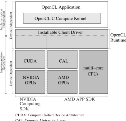
OpenCL. The Open Computing Languge (OpenCL) “is an open industry standard for pro-gramming a heterogeneous collection of CPUs, GPUs and other discrete computing devices or-ganized into a single platform” [Khronos Group, 2010, p.21]. Since 2008, OpenCL has the aim of becoming an open standard for heterogenous computing, including for GPGPU.

OpenCL is now managed by the Khronos Group [Khronos Group, 2008] and is supported by many companies and institutions. Up to the middle of 2012, there are 5 implementations of OpenCL:

• NVIDIA: NVIDIA GPU Computing SDK, for NVIDIA GPUs [NVIDIA Corp, d]

• AMD: AMD Accelerated Parallel Processing SDK, for AMD GPUs and multi-core CPUs

[AMD Inc, ]

• Apple: As a feature of operating system from Mac OS X v10.6, Snow Leopard [Apple Inc,] • IBM: OpenCL Development Kit, for PowerPC CPU [IBM,]

• Intel: Intel OpenCL SDK, for multi-core CPU [Intel Corp, a] The details of OpenCL will be presented in the next section.

6

NVIDIA announced CUDA in November 2006, released the first beta CUDA SDK in the first quater of 2007

7

(20)

Other languages. Another category of manycore programming solution try, like OpenMP, to mix regular Fortran, C/C++ code with directives, such as OpenHMPP8, and, more recently, OpenACC9_{. Other languages may be proposed in the following years as the field is rapidely}

evolving.

? ? ?

At the beginning of this thesis, in 2009–2010, we decided to use OpenCL since it was a promising standard. Indeed, we managed to run the same OpenCL code both on NVIDIA GPUs, on CPUs through the AMD SDK, and also (to a lesser extent) on some AMD GPUs (see on page 118). The following section will thus present in more the details the OpenCL architecture. However, many of these concepts can also apply to other existing languages (such as C CUDA) and potentially to future languages for manycore processors programming.

Remarks on C for CUDA. On the implementation of NVIDIA, it should be noted that both OpenCL and the progamming language “C for CUDA” function as a “device level programming interface” for the CUDA parallel computing architecture [NVIDIA Corp, 2009a]. The main difference is that while OpenCL interacts with the CUDA driver through the “OpenCL driver”, C for CUDA directly interacts with the CUDA driver.

C for CUDA is usually “ahead” OpenCL as it is designed specially for the NVIDIA GPUs, while OpenCL is an open standard, which is limited to common features of modern manycore processors. It means that, on the homogenous NVIDIA platform, OpenCL may not be as efficient as C for CUDA if the applications require advanced features such as the remote direct memory access (RDMA) between GPUs or the dynamic parallelism of CUDA 5 [Harris, 2012].

All the algorithms and data structures proposed in this thesis are implemented with funda-mental concepts. But when these algorithms and data structures are applied to a real application (see Chapter 6), some implementations with C for CUDA could be slightly more efficient. Nev-ertheless, we decided to keep OpenCL for his portability.

In general, we can say that C for CUDA benefits from specialized NVIDIA platforms, while OpenCL has the advantages of portability over heterogenous platforms.

1.2 Manycore high-performance computing with OpenCL

The OpenCL architecture consists of 4 models, which will be further discussed in the next sections:

• Platform model (Section 1.2.1): This section will describe the general architecture of an OpenCL compute platform as a host with one or multiple “computing devices”, and explain the hierarchy of the computing elements inside a device and the mapping of OpenCL platforms onto different processor architectures;

8

http://www.openhmpp.org/en/OpenHMPPConsortium.aspx

9

(21)

• Execution model (Section 1.2.2): This section will describe how a computing kernel can be run as multiple instances on the platform and explain the portability of an OpenCL program on different type of computing devices;

• Memory model (Section1.2.3): This section wll present different types of memory regions which can be used by an OpenCL program and describe how these regions are mapped onto the physical parts of the device;

• Programming model (Section1.2.4): This section will introduce data-parallelism and task-parallelism as two available programming models for the developement of OpenCL appli-cations.

Finally, Section1.2.5will explain some guidelines for efficient manycore programming. Again, these guidelines are not limited only to OpenCL and can be applied to any applications that run on current manycore processors.

OpenCL platforms used in this thesis. In order to clarify how the OpenCL standard run on heterogenous computing architectures from different vendors, we will use three examples: the NVIDIA’s Fermi generation GPUs [NVIDIA Corp, c], the AMD’s Evergreen generation GPUs

[AMD Inc, 2011b] and the Intel’s Nehalem microarchitecture CPUs [Semin, 2009]. These

selec-tions are consistent with the hardwares used for the experiments in this thesis: an NVIDIA GeForce GTX 480 GPU, an ATI Radeon HD5870 GPU and an Intel Xeon E5520 CPU.

This means that, on the five OpenCL implementations cited in page18), only the NVIDIA’s and the AMD’s implementations will be introduced and analysed (Figure1.3):

• NVIDIA implements the OpenCL standard as a “device level programming interface” for the CUDA parallel computing architecture [NVIDIA Corp, 2009a,NVIDIA Corp, 2012]. • AMD implements the OpenCL standard in the AMD Accelerated Parallel Processing SDK

(AMD APP SDK) [AMD Inc, 2011a], which supports both AMD GPUs and multi-cores CPUs from any vendor.

Comparing these three platforms in the light of the OpenCL architecture allows us to explain the difference of the hardware models between these GPU/CPU processors.

Remarks on the use of terminologies. Up to the mid 2012, the OpenCL standard is still being developped, so the terminologies may not be stable because different papers use differents terminologies. There are also differences between the documents of the same vendor. For exam-ple, in a technical white paper of AMD, published in june 2011, [AMD Inc, 2011c], the streaming core (SC) was considered as the processing element (PE). But in the AMD APP SDK OpenCL programming guide [AMD Inc, 2011a], published in december 2011, the SC is no longer consid-ered as the basic PE. Logically, the SC is further divided into other levels with each sub-SC containing which are considered as the PE.

In this thesis, the OpenCL specification of the Khronos Group [Khronos Group, 2010]10, the book “Heterogenous Computing with OpenCL” [Gaster et al., 2011], the AMD APP SDK

10

In november 2011, the Khronos Group released the OpenCL 1.2 specification, but all the implementation used in this thesis are based on OpenCL 1.1.

(22)

SDK Computing

NVIDIA AMD APP SDK

CUDA: Compute Unified Device Architecture CAL: Compute Abstraction Layer

Device Dependent

Device Independent

OpenCL Application OpenCL C Compute Kernel

GPUs CUDA NVIDIA AMD GPUs multi−core CPUs CAL

Installable Client Driver

OpenCL Runtime

Independent

Implementation

Implementation Dependent

Figure 1.3: OpenCL implementations on different platforms.

OpenCL programming guide [AMD Inc, 2011a], the paper of [Gummaraju et al., 2010] and the paper of [Zhang et al., 2011] are used as the main reference for the use of terminologies.

1.2.1 The OpenCL platform model

An OpenCL platform consists of a host connected to one or more compute devices, each of which contains one or more compute units. Each compute unit consists of one or more pro-cessing elements. This hierachical model gives an abstract logical view over an heterogenous and scalable computing system:

• The compute devices can be any kind of “processing units”, from different vendors, such as the Intel CPUs, the AMD GPUs, the NVIDIA GPUs, the AMD APUs, etc. Any compute device can be added to or removed from the computing system.

• The number of “cores” in each compute device can vary in a very wide range. Based on the design of the vendor and the hardware driver, the “core” can be further divided into processing elements. The scheduling and executing of the computing tasks in the compute units and the processing elements are transparent for the programmer.

The mapping of the OpenCL platform onto different architectures is based on both the physical and logical features of the devices. It depends also on the implementation approach of the SDK vendors. The mappings of the OpenCL platform onto Intel Nehalem microarchitecture CPUs, AMD Evergreen generation GPUs and NVIDIA Fermi generation GPUs are described in Figure1.4 and Table1.2:

(23)

Compute device Compute Unit Processing Element NVIDIA Fermi GPU Streaming

Multiproces-sor (SM)

Streaming Processor (SP, or CUDA core)

AMD Evergreen GPU SIMD Engine Processing Element

(PE) Intel Nehalem CPU Thread (Logical Core) Thread

Table 1.2: Mapping of OpenCL platform model onto Intel Nehalem CPU, AMD Evergreen GPU and NVIDIA GPU.

• Fermi GPUs, NVIDIA Computing SDK. An NVIDIA Fermi GPU contains upto 16 streaming multiprocessors. Each streaming multiprocessor consists of 32 “CUDA cores”. • Evergreen GPUs, AMD APP SDK. An AMD Evergreen GPU contains upto 20 SIMD

engines. Each engine consists of 16 stream cores, in each of which there are 5 processing elements. It means that there are 80 processing elements in an “AMD Evergreen SIMD engine”.

• Intel Nehalem CPUs, AMD APP SDK. At the physical view, there are upto 8 cores in an Intel Nehalem CPU. Thanks to the Intel’s Hyper-Threading Technology (HT)

[Intel Corp, 2002], it reaches 16 logical cores. In Intel’s offical technical specification

doc-uments, the HT based logical cores are called threads. In the OpenCL implementation of AMD APP SDK, the work-items are executed in turn by a thread (further presented in

1.2.2). This approach is the same with the Intel’s OpenCL implementation [Intel Corp, b]. Thus, for the Intel Nehalem CPUs, the thread is also the processing element.

At the physical view, the AMD SIMD engine is in the same level with the NVIDIA streaming multiprocessor, thus, the AMD stream core is comparable to the NVIDIA CUDA core. But as described above, the AMD stream core is further divided into a deeper level, while the CUDA core is not, even there are also 2 computational elements inside each CUDA core, the FP Unit and the INT Unit. The main reason for the difference between the logical view of the two vendors is that an AMD SIMD engine is a vector processor, where all processing elements can execute the same operation simultaneously on multiple data elements, while an NVIDIA streaming multiprocessors is a scalar processor where, at a point of time, either the FP Unit or the INT Unit is used to execute an instruction11_.

Thus, the difference in types of processor results in a signicicant difference between the numbers of “cores” in the technical specifications of the comparable GPUs of AMD and NVIDIA. For example, the ATI Radeon HD 5870 has 1600 “cores” while the NVIDIA GeForce GTX 480 has 480 “cores”, even these two GPUs seem to tie in the computing performance.

11

The multiprocessors of the NVIDIA changed from vector to scalar since the GeForce 8 series [NVIDIA Corp, 2006].

(24)

Man ycore high-p erformance computing with Op enCL 23 HOST

PE: Processing Element

SIMD: Single Instruction Multiple Data SC: Stream Core

PE: Process Element

T−PE: Transcendental Process Element

SM : Streaming Multiprocessor CC: CUDA Core

OPENCL Platform model (a) (b) (c) (d) Compute Unit PE PE PE PE Compute Unit PE PE PE PE Compute Device Compute Unit PE PE PE PE Compute Unit PE PE PE PE Compute Device SC SC SC SC SIMD Engine SC SC SC SC SIMD Engine PE PE PE PE T−PE Execution Branch Unit General − Purpose Register CC CC CC SM CC CC CC CC SM CC Thread (Logical Core) Thread (Logical Core)

AMD Evergreen GPU NVIDIA Fermi GPU

Intel Nehalem CPU

Result Queue Dispatch Port Operand Collector FP Unit INT Unit Instruction and Control Flow NVIDIA Computing SDK AMD APP SDK

Figure 1.4: (a) The OpenCL platform model. The mapping of OpenCL platform model onto (b) Intel Nehalem microarchitecture CPU, (c) AMD Evergreen generation GPU and (d) NVIDIA Fermi generation GPU. The architectures of the AMD stream core and the NVIDIA CUDA core are cited from [AMD Inc, 2011b] and [NVIDIA Corp, c].

(25)

1.2.2 The OpenCL execution model

An OpenCL program contains two parts: a host program that runs on the host and one or more kernels that runs on the compute devices. The host program aims to set up the OpenCL context and to provide the host-device interaction mechanism. The kernel will be run as a number of instances which are executing independently on the processing elements of the compute device.

The execution of an OpenCL program in the host side within the OpenCL context. The OpenCL context is an abstract container created on the host. A context can include one or more following resources: computing devices, command queues, memory objects, event object, program objects and kernels:

• Computing devices: as described in the platform model, a host connects to a set of computing devices. When creating a context, it must specify the list of selected devices from this set. An OpenCL context can be only created from the devices that belong to the same platform. In the case of multiple platforms co-existing in the machine, this heterogenous computing environment can be created and monitored by multiple contexts in the host program.

• Command queues: the OpenCL command queue is the mechanism which provides the interaction between host and devices. One command queue is associated with only one device, but one device can be associated with one or more command queues.

• Memory objects: the OpenCL memory objects are the “encapsulated container” pre-senting the data which can be transfered between the host and the device.

• Event objects: the OpenCL event objects are the mechanisms which allow the profiling of the submitted commands in the command queue and represent the dependencies between these commands.

• Program objects: the program objects represent the OpenCL C source code that can be compiled and run on the computing devices12. To avoid the confusion with the whole OpenCL program which consists of both the host program and the kernels, from now on, this part of source code will be called the kernel program. The OpenCL kernel program usually be compiled into the device specific instructions in the run time, allowing the execution in the heterogenous enviroment.

• Kernels: The OpenCL kernel is a function contained in the program and is a unit of execution that can be run on a device.

OpenCL provides a runtime layer called “installable client driver” (ICD). With the ICD, one can select, at runtime, a platform from heterogeneous computing environment (which may contain different OpenCL platforms from different vendors, Figure 1.3). An OpenCL program can be first compiled with one of these implementations, and the OpenCL APIs are linked only to the ICD13_{. When this program is launched, the host program can retrieve the list of platforms}

12

The OpenCL C programming language, used to implement the kernels that run on the computing devices, is based on the ISO/IEC 9899:1999 C language specification (C99 specification).

13

(26)

PTX: Parallel Thread Execution ISA: Instruction Set Architecture IL: Intermediate Language

Instructions Device Specific Itermediate Representation NVIDIA Computing SDK AMD APP SDK OpenCL C Kernel Source Code AMD GPU ISA x86 instructions NVIDIA GPU ISA IL PTX AMD GPU Multi−core CPU NVIDIA GPU

Figure 1.5: The compilation of OpenCL C Kernel on different platforms.

as well as the available devices in order to create the context. For each selected platform or device, the OpenCL program will transparently link to the dynamic library interface of the asscociated vendor’s SDK (Figure1.3)14.

The OpenCL kernel programs is built by the compiler of the selected vendor’s SDK. The kernel compilations on the AMD APP SDK and the NVIDIA Computing SDK are described in Figure 1.5. For x86 multi-core CPUs, the kernel program is compiled into the x86 instruc-tions. For AMD GPUs and NVIDIA GPUs, there are two compilation levels. First, the kernel program is compiled into an intermediate representation: AMD’s IL (Intermediate Language) or NVIDIA’s PTX (Parallel Thread Execution). This intermediate representation is further just-in-time (JIT) compiled into the device specific instruction set architecture (ISA), which will be run on the GPUs.

Generally, the execution of an OpenCL program has three main steps: (1) create the context, (2) compile the kernel program, (3) monitor the devices to do the computing works by submiting the commands (host-device data transfer, kernel execution, etc) to the command queue.

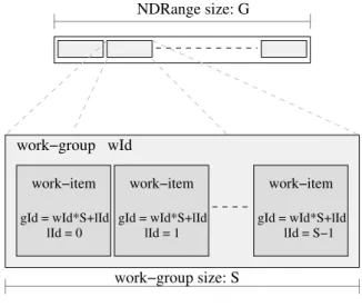
The mapping of the OpenCL kernel instances into the OpenCL index space. When the host submits a kernel to execute, the OpenCL runtime defines an N-dimensional index space called NDRange. The number of the dimensions of an NDRange can be 1, 2 or 3. An instance of the kernel, running on the computing device, is called a item. Each work-item, corresponding to one point in NDRange, executes the same code source on its given data. An NDRange of size G provides the execution space in which there are G work-items intended to be executed concurrently.

14

The NVIDIA GPU Computing SDK’s driver is provided in libCUDA.so. The ADM APP SDK’s driver is provided in liboclamd32.so and liboclamd64.so.

(27)

0000000000000000000 0000000000000000000 0000000000000000000 1111111111111111111 1111111111111111111 1111111111111111111 0000000000000000000 0000000000000000000 0000000000000000000 0000000000000000000 1111111111111111111 1111111111111111111 1111111111111111111 1111111111111111111 K4 K1 K3 K2 Command Queue 1 Device 1 Device 2 Command Queue 2 RunningK1 RunningK4 RunningK2 RunningK3 Time Context

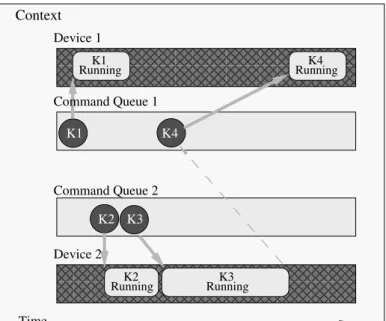
Figure 1.6: Example of the execution of an OpenCL program. An OpenCL context consists of 2 devices, associated with 2 command queues. The OpenCL program is a collection of 4 kernels: K1, K2, K3, K4.

K1, K2, K3 are independent from each other, except that K4 is dependent on K3. The kernels are submited and scheduled to run on the devices through the command queues. The event object associated with the submission of K3 maintains the dependency between K4 and K3 as well as the synchronization between the executions of the commands in different command queues.

At the view point on the whole index space, each work-item can communicate with the others in the global level. To support the local cooperations level, work-items are organized into work-groups. The data exchanges and the synchronizations between the work-items within the same work-group are simpler and more efficient than at the global level. Globally, the work-item and the work-group are assigned a unique identifier (ID). Inside the work-group, the work-item is also given the local ID.

The execution of the OpenCL kernel instances in the compute device. In both the NVIDIA Computing SDK and the AMD APP SDK, each work-group is mapped onto one compute unit, and one compute unit can host one or more work-groups. This means that each work-item is executed by one processing element, while one processing element may execute one or more work-items. At the device level, the execution of work-items on the GPUs and the multi-core CPUs are different.

The GPU compute unit schedules and executes the work-group as multiple sub-groups of N work-items. In the AMD APP SDK, these sub-groups are called the wavefronts and, in the NVIDIA Computing SDK, they are called the warps. The size of the wavefronts or the warps depends on the device. For example, the ATI HD 5800 series GPUs of the AMD Evergreen family contain the 64 item wavefronts and the NVIDIA Fermi GPUs contain the 32 work-item warps. The work-work-items in the same wavefronts or the same warps always execute the same instruction. Thus, the total number of the instructions needed to finish a kernel program increases linearly with the number of divergent code paths. A compute unit can support multiple

(28)

NDRange size: G work−group size: S work−group wId work−item lId = 1 gId = wId*S+lId work−item gId = wId*S+lId lId = S−1 work−item lId = 0 gId = wId*S+lId

Figure 1.7: Example of an 1-dimensional NDRange which contains G work-items, each with the unique global ID (gID) as well as the local ID (lID). The work-items are organized in work-groups of size S. Each work-group has a unique group ID (wID).

OpenCL CUDA

work-item thread

work-group thread-block

NDRange grid of thread-blocks

Table 1.3: The correlation between the execution model terminologies of the OpenCL standard and of the CUDA architecture

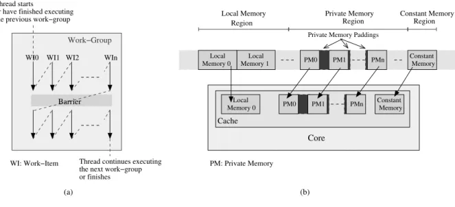
wavefronts/wraps simultaneously15. From now on, we use the notation warp to represent both the NVIDIA warp and the AMD wavefront, except the cases that need explicit distiguishment. For multi-core CPUs, the AMD APP SDK maps the whole work-group to one thread. Gener-ally, the kernel program can be divided into multiple sequential sections by the synchronization barriers. Each section is executed by each work-item in turn before changing to the next section. One thread can run multiple work-groups (Figure1.8a)16.

1.2.3 The OpenCL memory model

The OpenCL memory model is an abstract memory system with 4 distinct regions:

• Global memory is with full read/write access for all the work-items in the computing device. This region also plays the role of host-device data exchange.

• Constant memory is read-only accessible to all the work-items in the computing device. It is used for unchanged data that are written from the host and read simultaneously by

15

For exeample, the Streaming Multiprocessor of the NVIDIA Fermi GPUs can support upto 48 warps simul-taneously [NVIDIA Corp, b].

16

The more detail description of the OpenCL work-group execution by the CPU thread can be found in [Gummaraju et al., 2010, section 4.1] and [Gaster et al., 2011, Chapter 6].

(29)

Barrier

WI0 WI1 WI2 WIn

WI: Work−Item

Work−Group the previous work−group

or have finished executing Thread starts

or finishes the next work−group Thread continues executing

Constant Memory Local Memory 1 Local Memory 0 PM0 PM1 PMn Local PM0 PM1 PMn Constant Memory Cache Memory 0 Local Memory Region Region Constant Memory Private Memory Region Private Memory Paddings

PM: Private Memory

Core

(a) (b)

Figure 1.8: The AMD APP SDK implementation of OpenCL on multicore CPUs. (a): The execution of work-items of the work-group in the single thread. (b): The mappings of the local memory, private memories and constant memory associating to a work-group, from the main memory of the host to the cache inside the CPU core.

Global Constant Local Private

Host Dynamic allocation read/write Dynamic allocation read/write Dynamic allocation no access No allocation no access Kernel No allocation read/write Static allocation read-only Static allocation read/write Static allocation read/write

Table 1.4: Memory region - allocation and memory access capabilities (table cited from “The OpenCL Specifi-cation, version 1.1” of the Khronos Group [Khronos Group, 2010]).

all work-items.

• Private memory belongs to a work-item. This type of memory can only be accessed (read/write) by a work-item that owns it, and contains either variables declared inside the kernel codes or non-pointer arguments of the kernels.

• Local memory is assigned for a work-group and is shared among the work-items of this group. It can be dynamically allocated from the host program as the argument of the kernel or be statically allocated as a variable declared inside the kernel program. The host can not directly read from or write to this region: Only the work-items of the considered work-group can do the transfers between the local memory and the three other types of memory.

The mapping of the OpenCL memory platform onto each type of device depends on the memory system of the device and on the implementation of the vendor. For the GPUs, the global memory and the constant memory are mapped to the off-chip video memory of the GPUs. The private memory is usually mapped to the registers, but with the AMD GPUs, it

(30)

Compute Device

NVIDIA Fermi GPU AMD Evergreen GPU

Memory Private Element Memory Private Element Global Memory Processing Processing Compute Unit Constant Memory Streaming Multiprocessor Video Memory Register File Video Memory Register File SIMD Engine Local Memory

On−chip Memory Local Data Share

Figure 1.9: Mapping the OpenCL memory model (centre) onto NVIDIA Fermi GPU (left) and AMD Evergreen GPU (right). With AMD Evergreen GPUs, the private memory can be mapped on to either the registers or the video memory.

can be also mapped to the video memory (in the cases of private arrays and spilled registers [Gaster et al., 2011]).

The local memory on the GPUs of the two vendors is both mapped to the on-chip memory inside each compute unit17. For the AMD Evergreen GPUs, this type of memory is called “local data share” (LDS), inside each SIMD engine, and has the size of 32 KB. For the NVIDIA Fermi GPUs, the 64 KB on-chip memory inside each Streaming Multiprocessor is used to host both the local memory and the L1 cache.18.

Comparing to the off-chip memory, the on-chip memory is much larger in size, but has smaller bandwidth and higher latency.

The AMD APP SDK maps all types of OpenCL memory onto 4 continous distinct regions in the main memory of the host, outside the multi-core CPUs. But there are also mappings from local memory, the private memory and the constant memory regions in the main memory to the cache in each CPU core (Figure1.8b)19.

1.2.4 The OpenCL programming model

The host-device interactions through the command queues and the simultaneous execution of the kernel instances, as the work-items in the N-dimensional index space, allow the development of an OpenCL as the hybrid of 2 parallel programming models:

17

The on-chip memory inside the AMD Evergreen GPUs and NVIDIA Fermi GPUs is the scratchpad memory [Banakar et al., 2002]. It is also called the “programable cache”

18

The on-chip memory of the Fermi GPUs is configurable, the size of local memory and of L1 cache can be either (48 KB, 16 KB) or (16 KB, 48 KB).

19

The more detail descrition of mapping OpenCL memory model onto the main memory and the CPU caches can be found in [Gummaraju et al., 2010, section 4.2] and [Gaster et al., 2011, Chapter 6].

(31)

OpenCL CUDA

global memory global memory

private memory local memory

local memory shared memory

constant memory constant memory

Table 1.5: The correlation between the memory model terminologies of the OpenCL standard and of the CUDA architecture

• Data parallelism. • Task parallelism.

Data parallelism. At the global view, a kernel program is executed as a Single Program Multiple Data (SPMD) application: the same code is applied to different data. As one work-group is usually scheduled to run on one computing unit, one compute device can simultaneously process multiple work-units (instances of the kernel). However, as described in 1.2.2, the work-items that belong to the same wavefronts/warps always execute the same instruction, even if there are divergent code pathes20. It means that the execution of the work-items in the same wavefronts/warps follows the Single Instruction Multiple Data (SIMD) model.

The organization of the work-items into work-groups and the different levels of the memory model support multiple degrees of data parallelism. There following features of OpenCL should be noticed to achieve a good parallel strategy:

• The communications and synchronizations among the work-items in the same work-group are supported by the on-chip local memory and “barrier” OpenCL functions.

• Among the work-groups, the communications can only done by the out-chip global memory. • OpenCL does not support global synchronizations among work-groups.

So, it would better to implement the fine-grain parallelism on the work-items inside the same work-group, and the coarse-grain parallelism are on “inter-work-group” level.

Task parallelism. As an OpenCL kernel can be considered as one task, an OpenCL program is the form of a processing pipeline which consists of multiple tasks. The parallelism of the tasks and the multiple instances executing of the processing pipeline are shown in Section-1.1.1. The dependencies and the synchronizations between the tasks are defined and maintained by the event objects. There are two levels for processing the tasks simultaneously in the running time enviroment:

• Inter-device task parallelism: the tasks can be submitted to different compute devices to be processed parallely. For example, in Figure 1.6, two kernels K1 and K2 run parallely on Device 1 and Device 2.

20

(32)

• Intra-device task parallelism: In modern GPUs, multiple kernels can run concurrently in one compute device21. Depending on the global sizes of the kernels and the number of the processing elements, at one point in time, one or multiple kernels can be executed by the computing device.

1.2.5 Optimizing code for manycore OpenCL programming

This section discusses two factors that can significally influence the performance of an OpenCL application when running on GPUs: the global memory access and the branch divergence22. These two factors are analyzed and in particular cases which are further presented in Chapter-2, Chapter-3 and Chapter-4.

1.2.5.1 Branch divergence

As the running instance of the kernel code, a work-item consisits of multiple instructions that are dispatched to run on a processing element. In the GPU computing unit, the work-items are not processed independently but grouped into warps23. Moreover, the processing elements are also organized into the lanes. The scheduler at the computing unit level decides which instruction of which warp is executed by which lanes, thus the work-items belongs to the same warp always execute the same instruction simultaneously (as known as SIMD, Single Instruction Multiple Data).

In the run time, the data differences between the work-items can lead to different execution paths. This problem is called the branch divergence, and has a large impact on the per-formance of GPU applications, as all possible paths are dispatched sequentially to be executed. Having the SIMD behavior, the warp serially passes through all the available paths of the kernel code while disabling work-items that are not in each one. These work-items converge back when all the paths are completed [Lindholm et al., 2008] (Figure1.10).

Moreover, there is a waste in the use of processing elements: the total number of dispatched instructions is higher than the number needed to process them serially [AMD Inc, 2011a, Chap-ter 1].

1.2.5.2 Random global memory access

GPUs have a large off-chip memory, on which located the global memory, with high bandwidth but high latency (1.2.3)24. This type of memory is advantageous when the frequence of access transactions is small but the data amount of each transaction is large and in continuous region. As long as the memory access pattern is optimized, it can effectively handled hundreds or thousands simultaneous data read or write transactions [Jang et al., 2011]. But, in the case of high frenquency light weight memory accesses to the random region in the global memory,

21

For the NVIDIA GPUs, begin from the Fermi family, a GPU can execute the kernels in the same context concurrently [NVIDIA Corp, c, page 18].

22

The complete guides about optimization of OpenCL implementations on GPUs can be found in [NVIDIA Corp, 2009b] and [AMD Inc, 2011a].

23

As mentioned in page 26, the notation warp is used to represented both the NVIDIA warp and the AMD

wavefront.

24

The bandwidth and the latency of the GPU off-chip memory is compared with the main memory of the computer.

(33)

data

0 0 0 0 1 1 1 1 2 2 2 2 3 3 3 3

l id = get local id ;

if data[l id]%2 == 0 then computational-statment-1; else

computational-statment-2; end

for i = 0 to data[l id] do computational-statment-3; end

Figure 1.10: Example of branch divergence on a work-group of 16 work-items. get local id is the command to get the local identifier of the work-item in the work-group. All the work-items have to pass througth both paths in the conditional statement if-then-else and 4 iterations of the for-loop, even in each pass not all of them have to execute the corresponding computational statement.

it can cause the botleneck in data transfer due to the high latency and seriously decrease the performance of the application on the GPU. However, for the GPUs of NVIDIA Fermi or AMD Evergreen class, there is a cache for data transfer from the global memory.

As recommended in the OpenCL programming documents such as [NVIDIA Corp, 2009b, Chapter 3] or [AMD Inc, 2011a, Chapter 4], the global memory should be accessed in the coa-lesced pattern where the the work-items in the same wavefront/warp read from or write to the contiguous data elements. Moreover, the local memory, which is located in the very fast on-chip memory (1.2.3), should be used to temporarily store the computing data in order to reduce the number of global memory accesses.

Depending on the application and the size of the data, it is not always possible to apply these memory access optimizations. In this thesis, one of the key features of data structure design is to reduce as much as possible the number of random global memory accesses, which is the main idea of the neighborhood indexing approach, presented in Chapter-2. The use of local memory with coalesed data tranfer is also discussed in3.1.4.

1.3 GPU in Bioinformatics

The main purpose of this section is to list the bioinformatics applications that have been mapped onto GPUs. It can be considered as an extension from [Varr´e et al., 2011] with the addition of the bioinformatics GPGPU publications since 2009.

A note on speedups. In this section, we report many different studies from various fields of bioinformatics, with different methodologies for parallelizing, experimenting and evaluating the speedups. Moreover, the GPUs to do the experiments are also in the wide range and span several architecture generations. Generally, it is very difficult to fairly measure these speedups – for example, with GPU/CPU comparison, what is the base reference (CPU?, multi-core CPU? multi-multi-core CPU with SIMD instructions? grid of CPUs?), and was this CPU code

(34)

really optimized?

In addition, the raw times, in seconds, could be interpreted differently depending on the objective of application – for example, in our Chapter5, we will use a normalized measure for solving approximate pattern matching (see page 84). Finally, it lacks the independent bench-marking suite for these solutions. The speedups reported here should thus not be taken absolutely and should not be used to compare these different studies, but rather as a raw indication given by the different authors.

Contents of this section. Many bioinformatics high-performance studies concern sequence similarities: this domain was previously dominated by pairwise alignment (Section1.3.1), either by exact dynamic programming or with heuristics. With the advances in High-Throughput Sequencers (HTS), sequence similarities are now used in fruitful new domain of research (1.3.2). We also list other GPU studies in sequence algorithms (1.3.4), proteomics (1.3.5), data mining (1.3.6) and cell simulation (1.3.7).

? ? ?

Note that the motivation for studying similarities between genomic sequences will be pre-sented in the next chapter (page43), focusing on the core of this thesis – the filtering phase of seed-based heuristics.

The following pages do not aim to explain all cited problems, it is more a preview of what has already done with GPUs in bioinformatics – and what speedups the authors usually report.

1.3.1 Pairwise alignment

The tools presented here find similarities between two genomic sequences, either by exact dy-namic programming or, like in the rest of this thesis, within a seed-based heuristics.

1.3.1.1 Pairwise alignment by exact dynamic programming

Smith-Waterman. The main algorithm for computing local similarities between genomic sequences is Smith-Waterman [Smith and Waterman, 1981] which runs in quadratic time over the length of the sequences. This algorithm is very regular and was often parallelized in the three last decades on various platforms (dedicated hardware such as FPGA, CPU with SIMD, grids, etc) [Lavenier and Giraud, 2005]. One of the most efficient parallelizations of this algorithm should be the SIMD implementation of [Farrar, 2007], in which the author proposed an “striped query profile” technique to reduce the number of iteration loops over the dependent data. When running as a single thread on a 2.0 GHz Xeon Core 2 Duo, it achieved the speed about 3 billion cell updates per second.

The Smith-Waterman alorithm was thus an interesting target of choice for GPU paralleliza-tion. In 2006, [Liu et al., 2006b] proposed the GPU implementation of the algorithm by using OpenGL. The anti-diagonals of the dynamic programming matrix are processed simutaneously.

(35)

The implementation on a GeForce 7800 GTX has a reported speedup of almost 16× than OS-EARCH and 8× than SSOS-EARCH25. The first Smith-Waterman CUDA implementation should be the work of [Manavski and Valle, 2008] which was published in 2008. Their implementation on a single GeForce 8800 GTX was reported to be 3.5× to 4.7× faster than the experiments

of [Liu et al., 2006b]. In the same year, but some months later, [Munekawa et al., 2008]

pub-lished another CUDA Smith-Waterman implementation which also uses the anti-diagonal based parallelization strategy but with improved memory assigment and data reuse schemes. On a single GeForce 8800 GTX, the implementation of [Munekawa et al., 2008] was reported to be 3.1× faster than the one in [Manavski and Valle, 2008] and 6.4× faster than the one in [Liu et al., 2006b].

In 2009, [Striemer and Akoglu, 2009] also showed that [Manavski and Valle, 2008] was still highly CPU dependent. They proposed GSW, the absolute GPU dependent Smith-Waterman implementation. In comparison with the serial version of SSEARCH, GSW has a reported peak speed-up of 23× on a Tesla C87026. At the same year, [Liu et al., 2009a] released CUD-ASW++ which has a lot of memory access optimizations to gain the sequencing speed. More-over, there are two parallelization strategies in CUDASW++: the intra-task and the inter-task, which are used for the long and short queries respectively27. In comparision with the work of Manavski and Valle, on the same dual-GPU GeForce GTX 295, CUDASW++ had the speedup of up to 10×. In 2010, the same authors, [Liu et al., 2010b], released the upgraded version (CUDASW++2.0), with the optimized SIMT (Single Instruction Multi Thread) algo-rithm and the virtualized SIMD (Single Instruction Multi Data) vector programming model. On an NVIDIA GeForce GTX 295, CUDASW++2.0 was faster than CUDASW++ from 1.45 × to 1.72 ×. Independently, [Hains et al., 2011] showed that the intra-task kernel of CU-DASW++, which deals with the long queries, have a great impact on the overall perfor-mance of the genome database aligning and thus, they proposed their upgraded kernel. On an NVIDA C2050, the improved version of [Hains et al., 2011] increased the performance of at most 39.3. There were also other CUDA Smith-Waterman implementations in 2009 presented by

[Ligowski and Rudnicki, 2009] and by [Ling et al., 2009]. The peak performance of the

imple-mentation of [Ligowski and Rudnicki, 2009] on a dual NVIDIA 9800 GX2 was 4.1× higher than that of [Manavski and Valle, 2008] on a dual NVIDIA GeForce 8800 GTX. [Ling et al., 2009] did not focus on the running speed but on the length of the queries. In most cases, their imple-mentation was slower than those of [Manavski and Valle, 2008] and of [Munekawa et al., 2008] but it could align the sequence of any length28.

In 2010, [Dohi et al., 2010] (include all 3 authors of [Ling et al., 2009]) published the CUDA Smith-Waterman implementation with deeply optimizations on both algorithmics side and hard-ware side. In the peak performance, this implementation was about 1.45× faster than CUD-ASW++29. In this year, there was the first report of an OpenCL Smith-Waterman implemen-tation [Razmyslovich et al., 2010]. On an NVIDIA GeForce GTX 260, the authors announced

25

OSEARCH and SSEARCH are two Smith-Waterman implementations in the FASTA program

[Lipman and Pearson, 1988].

26

Striemer and Akoglu did not do the direct comparation between their works with the one in [Manavski and Valle, 2008]. They explained that the mapping in [Manavski and Valle, 2008] was the combination of CPU and GPU, and it could not align more than 400 residues on the GPU.

27_{In CUDASW++, the defaut threshold to differentiate long and short queries is 3072 residues.} 28

Both [Manavski and Valle, 2008] and [Munekawa et al., 2008] have the limit on the query length. On the testing platform of [Ling et al., 2009], the limits were 2500 and 2048 respectively.

29

It means that the performance of the implementation of [Dohi et al., 2010] is approximately equal to that of CUDASW++2.0