HAL Id: tel-03171103
https://tel.archives-ouvertes.fr/tel-03171103
Submitted on 16 Mar 2021HAL is a multi-disciplinary open access archive for the deposit and dissemination of sci-entific research documents, whether they are pub-lished or not. The documents may come from teaching and research institutions in France or abroad, or from public or private research centers.
L’archive ouverte pluridisciplinaire HAL, est destinée au dépôt et à la diffusion de documents scientifiques de niveau recherche, publiés ou non, émanant des établissements d’enseignement et de recherche français ou étrangers, des laboratoires publics ou privés.
SERS biosensors based on special optical fibers for
clinical diagnosis
Flavien Beffara
To cite this version:
Flavien Beffara. SERS biosensors based on special optical fibers for clinical diagnosis. Optics / Photonic. Université de Limoges, 2021. English. �NNT : 2021LIMO0009�. �tel-03171103�
University of Limoges
ED610 - Sciences et Ingénierie des Systèmes, Mathématiques, Informatique
(SISMI)
XLIM CNRS UMR-7252 Fiber photonics and coherent sources
Laboratory of Bio Optical Imaging, Singapore BioImaging Consortium, A*STAR
A thesis submitted to University of Limoges
in partial fulfillment of the requirements of the degree of
Doctor of Philosophy
High Frequency Electronics, Photonics and Systems
Presented and defensed by
Flavien BEFFARA
On January 11
th, 2021
Thesis supervisors:
JURY:
President of jury
Philippe Roy, CNRS Research director, XLIM Research Institute, Limoges, France.
Reporters
Marc Lamy de la Chapelle, Professor, Le M ans University, France.
Géraud Bouwmans, Professor, Lille University, France.
Examiners
Stefan Andersson-Engels, Professor, Tyndall National Institute, Cork, Ireland.
Guests
Fabrice Lalloué, Professor, Limoges University, France.
XLIM Research Institute:
Singapore BioImaging Consortium:
Dr. Georges Humbert
Dr. Dinish U.S
Dr. Sylvain Vedraine
Prof. Malini Olivo
Dr. Jean-Louis Auguste
SERS biosensors based on special optical fibers for clinical diagnosis
I dedicate this manuscript to my loved ones A. F. F. T.
Acknowledgments
First, I would like to acknowledge the Labex Sigma-Lim for funding half of my PhD. I would also like to acknowledge A*STAR Graduate Academy for funding the second half of my PhD. I thank Biomedical Research Council (BMRC), Agency for Science Technology and Research (A*STAR), Singapore and, the International Research Program “FiberMed” from CNRS, France for their contribution.
Second, I would like to thank the members of the jury who accepted to review this manuscript and attended the defense despite the difficult sanitary conditions due to Covid-19.
I would like to express my deepest gratitude to my two direct supervisors, Dr. Georges Humbert, in France, and Dr. Dinish U.S., in Singapore, for their guidance and support during these three years. The work presented here is the result of the very good synergy between XLIM and SBIC and more specifically between Georges and Dinish. I would like to thank both of them for allowing me to be a part of this project and for their countless advice during my PhD.
In France, I would like to extend my sincere thanks to Jean-Louis Auguste for his expertise and help during the fiber fabrication and the tapering sessions. A special thanks to Sylvain Vedraine for his help and the rich discussions we had on SERS and plasmon theory. Thanks should also go to Sébastien Rougier for the time he spent taking the SEM pictures presented in the following. I also wish to thank Maggy Colas and Julie Cornette for allowing me to use the Renishaw spectrometer at IRCER before I went to Singapore. Finally, I would like to thank the team and all the people who helped in a way or another during my stay at XLIM, this list is, of course, non-exhaustive: Philippe, Raphaël, Geoffroy, Baptiste, Romain, Marie Alicia, and all those I will inevitably fail to mention...
In Singapore, my deepest thanks go to Prof. Malini Olivo and Prof. Patrick Cozzone for welcoming me in SBIC and for their help and support to facilitate my return to France during the pandemic. ‘Merci
beaucoup’ to Douglas for his artistic advice, our discussions and most of all for making my stay in SBIC
so enjoyable. Special thanks to Jayakumar, Stephanie, Riazul, Amelia and Stanley for their numerous advice regarding the sample preparations and the handling of the spectrometer. Finally, I would also like to thank the entire LBOI group, Lunch Kakis and Beer group for welcoming me with open arms into their midst. I hope we will meet again soon.
On a more personal note, I must mention all my friends, from the start of my college years to those I met during my PhD. Citing all of them would be too long. Anyway, I wish to thank ‘les Ixeo’, ‘les
Matériaux’, ‘les Bios’, ‘les Profs’, ... for all the moments we shared during these eight years together.
These acknowledgments would not be complete if I did not mention the other PhD students: Étienne, Max, Lova, Gabin and Thomas for the daily jokes and laughs. This adventure would definitely not have been the same without them. Very special thoughts for Hugo and Matthieu who have been there for the past eight years, despite the distance. I am sure that we will keep saving kittens in the years to come. I am also extremely grateful to Nathalie, Ilona and Patrice for hosting me on my return from Singapore and for allowing me to work on my manuscript during the move. I cannot begin to express my thanks to my parents, Fabienne and Thierry, and my sister Astrid, for their unconditional love and support. They always believed in me and pushed me further even if they often did not understand what I was doing. The success of my PhD is undoubtedly thanks to them. Finally, I would also like to extend my deepest gratitude and love to Fiona, who followed me across the world and supported me daily, especially during the hardest moments. I could not have done all of this without her.
Rights
This creation is available under a Creative Commons contract:
« Attribution-Non Commercial-No Derivatives 4.0 International » online at https://creativecommons.org/licenses/by-nc-nd/4.0/
Table of Contents
Introduction ... 19
Chapter I. Introduction to Raman scattering and surface enhanced Raman spectroscopy ... 25
I.1. Introduction ... 25
I.2. Raman scattering ... 25
I.2.1. Discovery ... 25
I.2.2. Principle and application to Raman spectroscopy ... 25
I.2.3. Limitations ... 27
I.3. Surface enhanced Raman scattering (SERS) ... 28
I.3.1. Principle ... 28
I.3.1.1. Electromagnetic mechanism ... 28
I.3.1.2. Chemical mechanism ... 31
I.3.1.3. Wavelength dependence ... 31
I.3.1.4. Distance dependence ... 32
I.3.1.5. Total enhancement ... 35
I.3.2. Fabrication of SERS substrates ... 36
I.3.2.1. Principal parameters of a SERS substrate ... 36
I.3.2.2. Colloidal solutions of metallic NPs ... 38
I.3.2.3. Nanoparticles immobilized on planar substrates ... 39
I.3.2.4. Nanopatterning ... 42
I.3.2.5. Commercialized SERS substrates ... 45
I.3.3. Application of SERS substrates for biosensing... 46
I.3.3.1. Label free detection ... 46
I.3.3.2. Labeled detection ... 47
I.4. Conclusion ... 50
Chapter II. SERS-based optical fiber sensors ... 53
II.1. Introduction... 53
II.2. Photonic crystal fibers for SERS sensing ... 55
II.2.1. Solid-core photonic crystal fibers ... 55
II.2.2. Hollow-core photonic crystal fibers ... 56
II.3. Realizing SERS-active optical fibers ... 59
II.4. State-of-the-art in PCF SERS-sensing ... 61
II.4.1. Evaluation of the performance of SERS-based PCFs using common Raman tags ... 61
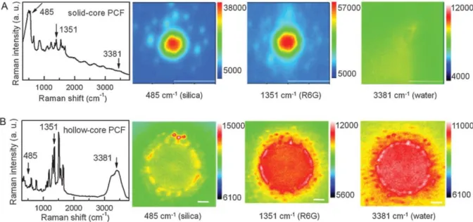
II.4.1.1. Illustration of the guiding mechanisms in solid and hollow-core PCFs ... 61
II.4.1.2. Effect of the fiber length on the SERS intensity ... 62
II.4.1.3. Limitations of hollow-core PCFs for SERS sensing ... 64
II.4.1.4. Improvement of the sensitivity of SERS-based fiber sensors ... 65
II.4.2. Biosensing with SERS-based PCFs ... 66
II.4.2.1. Label-free Raman detection ... 66
II.4.2.2. Label-free SERS detection ... 69
II.4.2.3. Labeled SERS detection ... 70
II.5. Discussion and conclusion ... 73
Chapter III. From basic simulation to detection of ovarian cancer biomarker with a SuC-PCF probe . 79 III.1. Determination of the optimum suspended core PCF parameters for SERS ... 79
III.1.1.1. Basic model used to approximate the final Raman intensity given by a suspended core
PCF ... 80
III.1.1.2. Simulation of the coupling efficiency between the laser and the fiber core ... 86
III.1.2. Fabrication of the different fibers ... 88
III.2. Optimization of the anchoring protocol ... 92
III.2.1. Presentation of the first developed protocol ... 92
III.2.1.1. Anchoring protocol ... 92
III.2.1.2. First Raman measurements ... 94
III.2.2. New protocol used to improve the sensitivity and reliability of the sensors ... 96
III.2.2.1. Presentation of the new protocol ... 96
III.2.2.2. Comparison between the two protocols ... 98
III.3. Comparison between injected and anchored gold nanoparticles ... 99
III.3.1. Description of injected gold nanoparticles ... 99
III.3.2. Comparison between both configurations ... 100
III.3.3. Core size study ... 102
III.4. Detection of relevant biomarker in clinical body fluids ... 104
III.4.1. Sensitivity and reliability of 3.5 µm core suspended core PCF from a different batch ... 104
III.4.2. Detection of haptoglobin in clinical cyst fluids ... 105
III.4.2.1. Protocol... 105
III.4.2.2. Results ... 107
III.5. Conclusion ... 109
Chapter IV. Ring core fibers, a novel fiber design for improving the sensitivity of SERS-based fiber sensors ... 113
IV.1. Observation on the limitation of sensitivity in SERS-based fiber sensors ... 113
IV.2. Simulation ... 113
IV.2.1. Adaptation of Chen’s model to the new design ... 113
IV.2.2. Comparison between the new design and the standard suspended core fiber ... 116
IV.3. Fabrication process ... 118
IV.4. Configurations used to excite the core and SERS sensing ... 124
IV.4.1. Envisioned solutions to properly excite the ring core ... 124
IV.4.2. Butt-coupling to multimode fiber ... 127
IV.4.2.1. Demonstration of light injection... 127
IV.4.2.2. SERS sensing with the multimode fiber and ring core fiber configuration... 129
IV.4.3. RCF taper ... 134
IV.4.3.1. Goal of the tapering ... 134
IV.4.3.2. Fabrication of tapered RCF ... 135
IV.4.3.3. Optical characterization ... 140
IV.4.3.4. SERS sensing with tapered ring core fiber ... 141
IV.5. Conclusion... 144
Conclusion and perspectives ... 149
Bibliography ... 152
List of Figures
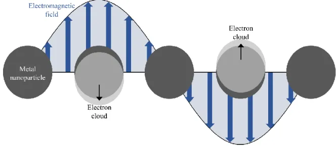
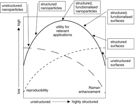
Figure 1 Schematic illustrating the two scattering phenomena occurring when a molecule is submitted to an electromagnetic field. ... 26 Figure 2 Simplified energy diagram illustrating Rayleigh, Stokes and anti-Stokes scatterings. ... 27 Figure 3 Illustration of the electron cloud delocalization undergone by a metallic nanoparticle when submitted to an electromagnetic field. ... 29 Figure 4 (a) SERS spectra measured when the molecules of pyridine are adsorbed on different
thicknesses of alumina, coated on AgFON. (b) Variations of the normalized SERS intensity of 1594 cm-1 peak of pyridine for the different alumina thicknesses. Reproduced from [60]. ... 33
Figure 5 Variations of the relative SERS intensity of the 2892 cm-1 peak of trimethylaluminum with
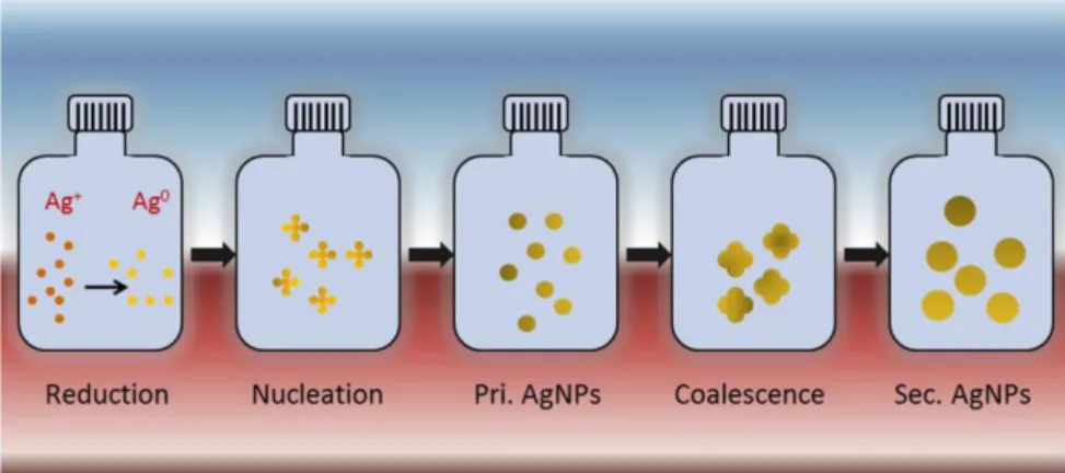
distance from a bare AgFON surface and AgFON functionalized with toluenethiol self-assembled monolayers. Reproduced from [61]. ... 34 Figure 6 Illustration of the mechanism that creates a giant increase of the EF in a hotspot. Reproduced from [69]. ... 34 Figure 7 Diagram showing the changing characteristics of SERS structures between the unstructured and highly structured variety. Reproduced from [82]. ... 36 Figure 8 Schematics presenting the notions of reproducibility and repeatability. A single substrate should exhibit uniform SERS signals under the same conditions, i.e. reproducibility. A batch of substrates prepared in the same conditions should exhibit identical SERS response, i.e. repeatability. 37 Figure 9 Representation of the chemical reduction process to synthesize colloidal Ag NPs. Silver ions (Ag+) form silver atoms (Ag) when they are submitted to chemical reduction. These atoms undergo
nucleation to form primary Ag NPs that further coalesce with each other to form final Ag NPs.
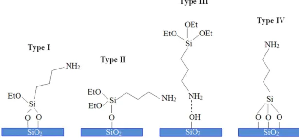
Reproduced from [88]. ... 38 Figure 10 Four possible orientations of APTES molecules on -OH terminated glass substrates.
Reproduced from [109]. ... 40 Figure 11 TEM micrographs of (a) The surface located band of silver nanoparticles in a cross section of the polycarbonate substrate. (b) A magnified section showing nanoparticles on the outside edge of the polymer. (c) A magnified section showing nanoparticles at the limit of furthest impregnation of the nanoparticles. Reproduced from [118]. ... 40 Figure 12 (a) SEM picture showing silver nanoparticles aligned along nanoripples on silicon. (b) Raman setup for polarized measurements. (c) Normalized intensity of the 1079 cm-1 band of MBN as a
function of θ obtained with 514 nm (green triangles) and the 647 nm (red squares) excitation. The respective solid lines correspond to fits of cos²(θ) (green) and sin²(θ) (red) function to the data.
Reproduced from [121]. ... 41 Figure 13 Schematic illustrating the screen printing process. Reproduced from [126]. ... 42 Figure 14 (a) Microscope picture showing the array of silica microsquares obtained by scanning horizontally and vertically a nanosecond laser on a silica substrate. (b) SEM pictures of the surface of a microsquare showing the silica NPs that resulted from the interaction with the laser. Reproduced from [127]. ... 43 Figure 15 SEM images of the nanowires arrays fabricated by Billot et al. Reproduced from [130]. ... 43
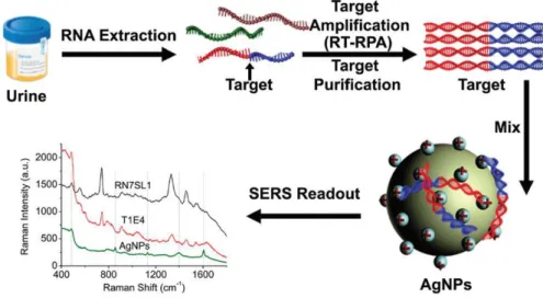
Figure 16 (a) Illustration of the single layer NSL. (b) Pattern of nanotriangles obtained with single layer NSL. Reproduced from [131]. ... 44 Figure 17 Different steps of NIL used by Ou et al. to fabricate nanofingers. Reproduced from [133]. 45 Figure 18 Process used to detect prostate cancer by extracting RNA from urine and measuring the SERS signal. Reproduced from [141]. ... 46 Figure 19 General steps needed to fabricate SERS nanotags. Reproduced and adapted from [149]. ... 48 Figure 20 Illustration of multiplex sensing using the MS technique. Reproduced from [20]. ... 49 Figure 21 Schematic representation of SERS (a) in a PCF and (b) on a planar substrate. Yellow
spheres: NPs, gray spheres: analyte molecules. The number of excited NPs and analyte molecules in (a) is much larger than that in the focus point of the laser in (b). ... 54 Figure 22 Cross-sections of (a) an SC-PCF, reproduced from [174], (b) a SuC-PCF, reproduced from [225], (c) a SiC-PCF, reproduced from [11], (d) a core-array PCF, reproduced from [180]. ... 55 Figure 23(a) HC-PCF. Reproduced from [184]. (b) Kagome PCF. Reproduced from [195]. (c) NANF. Reproduced from [196]. (d) LC-PCF. reproduced and adapted from [198]. ... 57 Figure 24 (a) Transmission spectra of a HC-PCF with a transmission window centered around 1060 nm when excited by a supercontinuum source and (b) of a HC-PCF with a transmission window centered around 1550 nm when excited by a tungsten lamp. The spectra were taken before (light gray) and after (dark gray) filling the holes of the HC-PCF with liquid D2O. The transmission window shift
is clearly visible for both fibers when the HC-PCF is filled. Reproduced from [189]. ... 58 Figure 25 (a) Schematic illustrating the injected configuration. 1: Mixing of analyte and NPs solutions. 2: Resulting mixture. 3: Withdrawing of the mixture with a syringe. 4: Injection of the mixture inside the PCF. 5: SERS measurement. (b) Schematic illustrating the anchored configuration. 1: Preparation of each solution and filling of the syringes. 2: Successive injection of the solutions inside the PCF. The molecules of APTES bind to silica (top), then the NPs bind to APTES (middle) and finally, the analyte molecules bind to the NPs (bottom). 3: SERS measurement. ... 60 Figure 26 Left: SEM pictures of the cross-sections of the two fibers used in the study by Han et al.. Right: illustration of the light guiding mechanisms in the SC-PCF and LC-PCF. Reproduced from [166]. ... 61 Figure 27 SERS spectrum and hyperspectral images measured at the end of (a) an SC-PCF and (b) a HC-PCF functionalized with Ag NPs and filled with an aqueous solution of R6G. Reproduced from [166]. ... 62 Figure 28 Variations of the Raman intensity of the 1351 cm-1 peak of R6G with the fiber length, for
several NPs coverage density. The presented results were obtained in (a) an SC-PCF and (b) a HC-PCF. Reproduced from [166]. ... 63 Figure 29 (a) Experimental variation of the SERS intensity with the fiber length for 50 nM of R6G. Inset: measured spectra for the different SiC-PCF lengths. (b) Simulated variations of the relative SERS intensity with fiber length for several concentrations of Au NPs in backward collection setup. Reproduced from [11]. ... 64 Figure 30 (a), (b), (c) SEM pictures of the three fibers used by Oo et al. in their study. (d), (e) and (f) simulated electric field distribution of the fundamental mode when the three fibers are filled with ethanol. Reproduced from [201]... 65
Figure 31 Calculated mode profile for a 785 nm laser coupled (a) in the solid core of an SC-PCF and (b) with an offset, in the cladding. Reproduced from [183]. ... 66 Figure 32 (a) Raman spectra obtain for different concentrations of heparin. Inset: zoom-in on the 1005 cm-1 peak for the lowest concentrations. (b) Intensity of 1005 cm-1 peak measured for each
concentration. Reproduced from [200]... 67 Figure 33 Raman spectra of (a) glucose, (b) fructose and (c) mixture of glucose and fructose.
Reproduced from [203]. ... 67 Figure 34 Transmission spectra of commercial HC-PCF when the core is empty and when it is
selectively filled with water. The purple dashed line represents the ideal transmission spectrum with step index guidance. Reproduced from [206]. ... 68 Figure 35 (a) Schematic illustrating the setup used for gas detection with SERS-based PCF probes. (b) Raman spectrum of the mixture of toluene, acetone and 111-trichloroethane obtained with a HC-PCF. Reproduced from [17]. ... 69 Figure 36 SERS and Raman spectra of adenosine in cuvette and in HC-PCF. Reproduced from [210]. ... 70 Figure 37 Top: Schematic presenting a SERS nanotag. The little blue circles represent the Raman reporter. Bottom: Representation of multiplex detection inside a HC-PCF with three nanotags.
Reproduced from [5]. ... 70 Figure 38 Raman spectra of Cy5, MGITC and mixture containing Cy5 and MGITC illustrating the possibility to obtain multiplex detection. Reproduced from [5]. ... 71 Figure 39 (a), (b) and (c) Representation of the formation of sialic acid/DBA complex. (d) Raman spectrum detected from DBA tagged cells in SiC-PCF. (e) Schematic illustrating the detection of sialic acid at the surface of HeLa cells in SiC-PCF. Reproduced from [12]. ... 72 Figure 40 (a) Design of the SuC-PCF that should have been used in the simulation to fit more closely to real fibers. (b) Schematic of the ideal case of a silica rod surrounded by the effective layer and immersed in water. This design was used in the simulation to approximate the design of the SuC-PCFs. 1 represents the silica core (gray), 2 represents the effective layer (yellow) and 3 represents water (blue). The dashed circle in (a) represents the core simulated in (b). ... 82 Figure 41 (a) Fundamental mode simulated for a 1 µm rod surrounded by the effective layer and water. (b) Zoom in the core area: the core, the effective layer and the beginning of the water layer are visible. The color scale is applicable for (a) and (b). ... 83 Figure 42 Variations of the calculated 𝑓𝑅𝐼 with the core radius for 10 cm long SuC-PCFs covered with 0.05 𝑁𝑃𝑠/µ𝑚2 ... 84 Figure 43 Variations of the calculated 𝑓𝑅𝐼 with the core radius for 10 cm long SuC-PCFs and different NPs coverage densities. ... 84 Figure 44 (a) Variation of the calculated 𝑓𝑅𝐼 with the core radius for 1 mm long SuC-PCFs and different NPs coverage densities. Comparison of the calculated 𝑓𝑅𝐼 for 1 mm and 10 cm SuC-PCFs for (b) 𝐶𝐷 = 0.01 𝑝𝑎𝑟𝑡𝑖𝑐𝑙𝑒/µ𝑚2and (c) 𝐶𝐷 = 1 𝑝𝑎𝑟𝑡𝑖𝑐𝑙𝑒/µ𝑚2. ... 85 Figure 45 (a) Design of the simulated SuC-PCFs with different core sizes, and zoom-in on the 2D distribution of the Poynting vector of the fundamental mode propagated in a core diameter of 3.5 μm (superimposed in light gray). (b) Distribution of the center of a Gaussian beam (corresponding to the laser beam from the Raman spectrometer) randomly positioned (250 times) within an area limited by a
circle of 0.5 μm radius around the center of the fiber. (c) Normalized coupling coefficients between the Gaussian beam (following the positions in, (b)) and the fundamental mode of SuC-PCFs with different core sizes. (d) Calculated maximum and average coupling coefficient values from the values plotted in, (c). SD in average coupling coefficient is denoted with red lines (reproduced from [225]. 87 Figure 46 (a) Schematics of the different steps realized during the stack-and-draw process, in brackets is given the order of magnitude of the diameter. (b) Zoom-in on the preform step to define the
parameters used in the calculation made to select the different tubes. ... 89 Figure 47 Schematics illustrating the pressurizing system used during the drawing of (a) the cane and (b) the preform. The blue sections represent the closed capillaries. Practically, we collapsed the end of the capillaries by torching them. P- and P+ represent respectively the vacuum and the overpressure
applied in the different sections of the cane and preform. ... 90 Figure 48 SEM pictures of fabricated SuC-PCFs with different core sizes. (a) 0.9 µm. (b) 1.1 µm. (c) 1.4 µm and (d) 3.5 µm. ... 91 Figure 49 Schematic illustrating the locations where the power was measured to determine the
coupling loss of a SuC-PCF. ... 92 Figure 50 (a) Presentation of the dimer: a represent the radius of the two NPs and g the gap between them. The excitation light is polarized along the main axis. (b) Extinction coefficient as a function of the wavelength for a single NP and for the dimer (with different gaps). SERS enhancement factors for different gaps between the two NPs and for a single NP. Dashed line represents the SERS
enhancement averaged over the entire metallic surface for a dimer with g=2 nm. Reproduced from [19]. ... 93 Figure 51 (a) Representation of an APTES molecule. (b) Schematics illustrating Au NPs anchored on the walls of a SuC-PCF. Zoom: illustration of one of the configurations in which APTES and Au NPs bind to silica. (c) Schematic showing the setup used to pump liquids inside the fiber holes Zoom: illustration of the needle/SuC-PCF assembly. ... 94 Figure 52 Schematic illustrating the main components of the Raman spectrometer used for the
measurements. ... 95 Figure 53 (a) Signature spectrum of ATP. The two main peaks are located at 1080cm-1 and 1590 cm-1.
Inset: Structure of ATP bound to an Au NP through its thiol group. (b) Normalized SERS intensity of the 1080 cm-1 peak of ATP for the two ends of two 3.5 µm core SuC-PCFs. The error bars represent
the SD measured between the seven spectra per end. ... 96 Figure 54 (a) Schematic illustrating the broken SuC-PCF that allowed us to take the pictures of the inner wall of the fiber. (b), (c), (d) SEM pictures of the inner wall of a SuC-PCF with Au NPs
anchored using the new protocol at different magnifications. ... 97 Figure 55 Normalized SERS intensity of the 1080 cm-1 peak of ATP for the two ends of two 3.5 µm
core SuC-PCFs using the long anchoring protocol. ... 97 Figure 56 (a) Comparison of the effect of the short and long anchoring protocols on the normalized SERS intensities of the 1080 cm-1 peak of ATP at the free end of two 3.5 µm core SuC-PCFs. (b)
Same comparison made at the needle end of the same fibers. ... 98 Figure 57 Variations in SERS intensity of ATP peak at 1080 cm-1 with the concentration of injected
Au NPs for fibers with 0.9 μm, 1.4 μm and 3.5 μm core; error bars represent the standard deviation across 8 measurements obtained with the same fiber. ... 100
Figure 58 For each core size, comparison between the injected and anchored configurations of (a) the average SERS intensity at 1080 cm-1; error bars represent the standard deviations across two or three
samples, (b) the calculated average RSD in reproducibility, (c) the calculated average RSD in
repeatability. ... 101 Figure 59 Black curve: variation of average SERS intensity of the 1080 cm-1 peak of ATP, in the
anchored configuration, for 0.9 µm, 1.4 µm and 3.5 µm core SuC-PCFs. The error bars represent the standard deviation calculated for three fibers per core size. Gray curve: variation of the simulated 𝑓𝑅𝐼 with the core radius of 10 cm long rods with 30 particles/µm². ... 102 Figure 60 (a) Variations in the Raman intensity of 1080 cm−1 peak (14 measurements) from the SuC-PCF showing the excellent reproducibility of the sensor, error bars represent the SD of the 14 measurements. Inset: Acquired 14 spectra from one of the representative fibers. (b) Variations in the Raman intensity of 1080 cm−1 peak from six different fibers showing the good repeatability, error bars represent the SD of 14 measurements acquired for each fiber; Inset: individual spectrum from six different fibers. (c) Calibration curve of Raman intensity with ATP concentration showing the good linearity of the sensor, error bars represent the SD obtained from 14 measurements. Reproduced from [225]. ... 105 Figure 61 (a) Schematic of the functionalization process inside the holes of the PCF for biomarker sensing. (b) Coupling of the light from the objective lens of the Raman spectrometer and
backscattering collection of the signal from the fiber end. Zoom-in on the fiber end face and holes with the attached protein and read out Raman tag. Reproduced from [225]. ... 106 Figure 62 (a) SERS spectra of the bare fiber, the fiber after anchoring with APTES and after adding AB-ATP that binds to Hp biomarkers demonstrating the specificity. All prominent peaks of ATP are observed. (b) Normalized Raman intensity of 1080 cm−1 peak from clinical OCF having different stages of cancer. ****P<.0001 denotes significance when compared to patient A. (c) Normalized Raman intensity of 1080 cm−1 peak from the second set of clinical OCF depicting different stages of cancer. ****P<.0001 denotes significance when compared to patient D. Reproduced from [225]. ... 108 Figure 63(a) Schematic of the RCF design used for the simulation. (b) Design simulated in chapter III for a 3.5 µm rod. The core size in (a) and (b) are true-to-scale to have a better visualization of the surface increase. 1 represents the silica core (gray), 2 represents the effective layer (yellow, thickness not true-to-scale) and 3 represents water (blue). ... 114 Figure 64 Simulated Poynting vectors of the first five simulated modes with decreasing values of neff
obtained with Dcore= 25 µm, tcore = 0.5 µm and CD = 0.05 particles/µm² ... 116
Figure 65 (a) Calculated factor proportional to the SERS intensity for increasing diameters of the ring and the best SuC-PCF with CD = 0.05 particles/µm² and tcore = 0.5 µm. (b) Comparison between
calculated proportional factors for two CDs and for Dcore = 25 µm and tcore = 0.5 µm. (c) Comparison
between calculated proportional factors for two ring thicknesses and for Dcore = 25 µm and
CD = 0.05 particles/µm². ... 117 Figure 66 Schematics illustrating the pressurizing system used during the first attempts of (a) the cane and (b) the fiber drawings. The blue sections represent the closed capillaries. P- and P+ represent
respectively the vacuum and the overpressure applied in the different sections of the stack and
preform. ... 119 Figure 67 Pictures of the cane obtained for different values of vacuum applied between the jacket tube and the stack with closed capillaries: (a) vacuum = -2 kPa, (b) vacuum = -5 kPa, (a) vacuum = -3 kPa. ... 120
Figure 68 SEM pictures of (a) RCF 1, (b) zoom-in on the ring core, (c) RCF 2 and (d) zoom-in on the ring core. The open apices are visible on (b) and (d). The scale bars represent respectively (a) 100 µm, (b) 20 µm, (c) 200 µm and (d) 30 µm. ... 121 Figure 69 New pressurizing system used to fabricate the cane. The blue sections represent epoxy glue. ... 122 Figure 70 Zoom-in on the ring of the RCF with closed apices. ... 122 Figure 71 SEM pictures of (a) RCF 3 (outer diameter of 600 µm), (b) zoom-in on the ring core, (c) RCF 4 (outer diameter of 580 µm) and (d) zoom-in on the ring core. The open apices are visible on (b) and (d). The scale bars represent respectively (a) 200 µm, (b) 40 µm, (c) 200 µm and (d) 40 µm. ... 123 Figure 72 SEM picture presenting an open apex between the ring core and the struts holding it in place. The scale bar represents 2 µm. ... 124 Figure 73 Picture of the output of an RCF excited by focusing the laser directly using 5x objective lens. ... 124 Figure 74 (a) Picture of the entry face of the RCF. (b) Output distribution of the light when the laser is focused on the circle of (a). ... 125 Figure 75 Signature SERS spectrum of 2-NT. ... 126 Figure 76 SERS intensity measured on the six apices of a single RCF. The error bars represent the variations measured across the four spectra for a single apex. ... 126 Figure 77 Schematic illustrating the principle of RCF excitation using a MMF. ... 127 Figure 78 Pictures of (a) the RCF with open apices excited by a MMF, (b) the output distribution of the light at the end of the RCF, (c) the fiber with closed apices and (d) the distribution of the light at the end of this fiber. ... 128 Figure 79 Schematic illustrating the locations where the power was measured to estimate the coupling loss from MMF towards RCF and from RCF towards MMF... 129 Figure 80 (a) SERS spectra obtained by exciting the RCF with a MMF (dark) and by directly focusing the laser on one apex (gray). (b) SERS spectra obtained by exciting the RCF with a MMF for larger laser power than in (a) (dark) and ATP signature spectrum (gray). ... 130 Figure 81 (a) Silica Raman signal measured using 70 cm long MMF. (b) Variation of the Raman intensity of the 480 cm-1 peak of silica for different lengths of MMF. ... 131
Figure 82 SERS spectrum of 2-NT collected with an RCF using the MMF configuration (black), same spectrum after removing the silica background (dark gray) and signature spectrum of 2-NT (light gray). ... 132 Figure 83 Average SERS intensities of the 2-NT 1380 cm-1 peak measured using different MMFs to
excite RCF 1. The error bars represent the standard deviation between the 10 measurements acquired to calculate the average intensity. ... 133 Figure 84 Comparison of the SERS intensities measured with RCF 1 and 3.5 µm core SuC-PCF. The experiment was repeated four times to ensure the authenticity of the results. The error bars represent the standard deviations measured over the ten spectra acquired per fiber. ... 133 Figure 85 Schematic illustrating the principle of the direct excitation of the RCF with (a) an un-tapered end and (b) a tapered end. The figures on the right represent the un-tapered face of the RCF with the expected field distributions. ... 135
Figure 86 Schematic presenting the preset parameters used to fabricate the RCF tapers. ... 136 Figure 87 Fabricated tapers with long heating time. The structure is almost entirely collapsed... 137 Figure 88 Fabricated taper of the fiber with closed apices with Dwaist = ~200 µm. ... 137
Figure 89 Schematics illustrating the setup used to apply (a) overpressure in the external holes of an RCF during tapering and (b) vacuum only inside the center hole. The blue sections represent epoxy glue. ... 138 Figure 90 Fabricated taper of fiber with closed apices with Dwaist = 100 µm and with vacuum applied
in the center hole. ... 139 Figure 91 (a) and (c) SEM pictures representing two tapers fabricated using RCF 4 when withdrawing -0.7 mL of air inside the center hole (b) and (d) Zoom-in on the core region for each taper. ... 140 Figure 92 Distribution of the field at the output of an RCF with a core diameter of 89 µm (RCF 4) for several excitation techniques. (a) Tapered RCF, (b) direct focus with 10x objective lens and (c) MMF excitation. ... 141 Figure 93 Measured SERS spectra of ATP under normalized conditions using a tapered RCF (black curve) and a 3.5 µm core SuC-PCF (gray curve). We offset the two spectra for more readability. ... 142 Figure 94 SERS spectra measured under fixed experimental conditions with the 3.5 µm core SuC-PCF and a tapered RCF ... 143
List of Tables
Table 1 Percentage of light in each layer of four SuC-PCFs with different core sizes. ... 83 Table 2 Parameters of the fabricated SuC-PCFs measured with a SEM ... 91 Table 3 Measured average SERS intensity, calculated average reproducibility and calculated average repeatability in anchored and injected configurations for 3 core size SuC-PCFs ... 101 Table 4 Histology and CA 125 results from OCF samples collected in five patients ... 108 Table 5 Percentage of evanescent field in every section of the simulated ring suspended in water ... 115 Table 6 Percentage of evanescent field in every section of the simulated ring suspended in water when tcore = 1.1µm ... 118
Table 7 Parameters of the first RCFs drawn during my PhD ... 120 Table 8 Parameters of the second set of RCFs drawn during my PhD. The strut thickness was too thin to be measured precisely so we do not present their dimensions here ... 123 Table 9 Parameters of the real SuC-PCF and RCF used to simulate their estimated 𝑓𝑅𝐼 ... 134 Table 10 Parameters of the tapers fabricated from RCF 4. The core of taper 2 was too thin to be measured precisely so we do not present its dimensions here ... 140 Table 11 Powers measured to estimate the coupling loss of a tapered RCF and 3.5 µm core SuC-PCF ... 141 Table 12 Measured SERS intensities of the 1080 cm-1 peak of ATP for a 3.5 µm core SuC-PCF and
tapered RCF ... 142 Table 13 Measured average SERS intensities of the 1080 cm-1 peak of ATP and simulated f
RI for a 3.5
Abbreviations
2-NT 2-naphthalenethiol
4-MBA 4-mercaptobenzoic acid
4-MBT 4-methylbenzenthiol
A1AT Alpha-1-antitrypsin
AB Antibody
AFP Alpha-fetoprotein
Ag NPs Silver nanoparticles
AgFON Bare silver film-over-nanosphere
ALD Atomic layer deposition
APTES (3-Aminopropyl)triethoxysilane APTMS (3-Aminopropyl)trimethoxysilane
ATP 4-aminothiophenol
Au NPs Gold nanoparticles
BSA Bovine serum albumin
CCD Charge coupled device
CD Coverage density
CH Cumene hydroperoxide
CM Chemical mechanism
Cy5 Cyanine5
DBA 4-(dihydroxyborophenyl) acetylene
EBL Electron beam lithography
EDC 1-éthyl-3-(3-diméthylaminopropyl)carbodiimide
EF Enhancement factor
EGFR Epidermal growth factor receptor ELISA Enzyme-linked immunosorbent assay
EM Electromagnetic mechanism
FEM Finite element method
HC-PCF Hollow-core PCF
Hp Haptoglobin
LAA Linoleamide alkyne
LC-PCF Liquid core PCF
LOD Limit of detection
LSPR Localized surface plasmon resonance
MBN 4-mercaptobenzonitrile
MFON Metallic film over nanosphere MGITC Malachite green isothiocyanate
MMF Multimode fiber
MPTMS (3-Mercaptopropyl)trimethoxysilane
MS Molecular sentinel
NANF Nested anti-resonant nodeless fiber
NHS N-hydroxysuccinimide
NIL Nanoimprint lithography
NIR Near infrared
NP Nanoparticle
NSL Nanosphere lithography
OCF Ovarian cyst fluid
PBG Photonic band gap
PBS Phosphate buffer saline
PCF Photonic crystal fiber
PCR Polymerase chain reaction
PET Polyethylene terephthalate
PNBA P-nitrobenzoic acid
R6G Rhodamine 6G
RCF Ring core fiber
RhB Rhodamine B
RSD Relative standard deviation
SC-PCF Solid-core PCF
SD Standard deviation
SEM Scanning electron microscopy
SERS Surface enhanced Raman spectroscopy SHIN Shell isolated nanoparticles
SHINERS Shell isolated nanoparticle enhanced Raman spectroscopy
SiC-PCF Side-channel PCF
SMF Single mode fiber
SuC-PCF Suspended core PCF
TEM Transmission electron microscopy
TERS Tip enhanced Raman spectroscopy
TIR Total internal reflection
Introduction
Biochemical sensing in general is an important research domain that has tremendous applications in various disciplines such as environmental monitoring, food industry, homeland security and healthcare. In this manuscript, we focus on the latter and more precisely on the detection of severe diseases. To this day, countless patients are still dying from cancer, neurodegenerative disorders, and so on. Therefore, new sensors are still in need to facilitate early diagnosis to start the treatment as soon as possible and improve the survival rate of the patients. In this context, traditional tissue biopsy still represents the gold standard in many diagnoses. It consists of taking a portion of tissue to determine the stage of a disease. Unfortunately, diseases like cancer are constantly evolving and tissue biopsy only gives an insight on the disease stage at the time of the sampling. Since this technique is invasive, it cannot be repeatedly performed. Thus, monitoring periodically the evolution of the disease and the effect of the treatment becomes arduous. Recently, another form of biopsy, called liquid biopsy, has emerged. This technique aims to detect a disease by identifying biomarkers in body fluids, such as blood, saliva, urine, ascites and cerebrospinal fluid. The target biomarkers take many forms. For instance, in the detection of cancer, the biomarkers can be circulating tumor cells, DNAs and non-coding micro-RNAs, extracellular vesicles or proteins. Circulating tumor cells are cells that have entered the circulatory system after having been separated from the tumor tissue. Circulating tumor DNAs and non-coding micro-RNAs are genetic content of the cancerous cells that can enter the circulatory system after a cell apoptosis (death) for example. Similar to healthy cells, tumor cells also secrete extracellular vesicles, such as exosomes, to communicate with their surroundings. These vesicles can contain protein, lipids or genomic material that reveal the state of the original cell. All these biomarkers are present in body fluids, and their concentration may be linked to the disease stage. They can also be used to monitor the efficiency of treatment. This technique is much less invasive compared to biopsy tissue and can thus be used more regularly in order to evaluate the evolution of the disease or the efficiency of the treatment. Unfortunately, body fluids are very complex mixtures and detecting trace amount of a target biomarker can be extremely challenging.
Among the techniques that could allow detecting the biomarkers, Raman spectroscopy presents several advantages. It allows characterizing the chemical nature, chemical structure as well as the orientation of many analytes. In addition, the sharp signature peaks of Raman scattering allow multiplex detection, which can be useful for studying complex fluids. This technique is based on the interaction of an excitation light with an analyte, and for a long time, it has been neglected due to the extremely low intensity of the Raman signal. However, the discovery of surface enhanced Raman spectroscopy (SERS) and the development of nanoscience helped in democratizing this sensing technique. It was demonstrated that nanoparticles (NPs) made of noble metal were able to enhance locally both the excitation light and the Raman signal, resulting in enhancement factor ranging from 106 to 1011. This
allowed overcoming the main limitation of Raman spectroscopy while preserving the fingerprint spectra of the molecules. Even though single molecule sensing was reported under constrained conditions, current substrates still lack sensitivity and reliability for real-life applications. Nanopatterning helped in improving the sensitivity and reliability of state-of-the-art SERS substrates. Nevertheless, there is still a great demand for improved sensitivity and reliability, especially for the detection of biomarkers in clinical bio fluids.
A solution could be to use optical fibers as substrates. Indeed, they are known for their compactness, and their flexibility. In addition, they allow for a low-loss guiding of the light in their core. A special class of fibers, i.e. photonic crystal fibers (PCFs), possess holes that run along their entire length. These holes allow for the incorporation of liquid or gas inside the fiber. Therefore, PCFs represent an ideal candidate for SERS sensing since they exhibit the advantages of optical fibers while allowing for a
potential larger surface of interaction between the light and the analyte. Indeed, since the analyte is inside the sensing medium, the light can interact with it for relatively long lengths. This increased interaction surface area results in an increased sensitivity. In addition, since the light can interact with a much larger number of NPs along the fiber length, PCFs should also improve the reliability of planar substrates, which is currently limited by the precision of nanofabrication techniques. In summary, SERS-based PCFs feature the remarkable advantages of optical fibers while preserving the great identification properties of SERS. In this context, they should simultaneously improve the sensitivity and the reliability of SERS sensors while being compatible with the development of optofluidic platforms with one-step collection/readout processes. All these interests could help in overcoming the remaining limitations that currently forbid SERS for advancing as the gold standard in many biosensing procedures.
The Laboratory of bio-optical imaging (LBOI) from Singapore BioImaging Consortium (SBIC), A*STAR, is specialized in bio-imaging and optical sensing. They develop photoacoustic imaging devices [1] and innovative Raman spectroscopy techniques [2,3]. A few years ago, they started studying the interest of optical fibers for SERS biosensing. Using commercial PCFs, they achieved multiplex detection of cancer biomarkers [4,5]. However, this type of fiber was not specifically designed for SERS sensing and a fiber specifically fabricated for this application could have helped in improving the results further. On the other hand, the team Fiber photonics in XLIM research institute, a joint research unit between CNRS and the University of Limoges (France), is specialized in the fabrication of optical fibers. They develop specialized optical fibers for various applications, such as high-power lasers [6,7], ultra-short pulsed lasers [8,9] and sensing [10]. Thus, a collaboration between SBIC and XLIM to fabricate specifically designed SERS-based fiber sensors appears logic and meaningful. In this context, they developed a novel design of PCF that improved by three orders of magnitude the detection of Rhodamine 6G (R6G) [11]. They also demonstrated the potential of this fiber for biosensing by detecting 2.5 fmol of sialic acid at the surface of a single cell while previous reported techniques required 105 cells
[12]. Based on these very promising results, they obtained a joint grant for a PhD student to further improve their SERS-active fiber probes. I began my PhD in XLIM to fabricate new optical fibers, which parameters have been specifically designed to improve SERS sensing and I spent the other half of my PhD at SBIC, in Singapore, to realize biosensing experiments with the fabricated fibers. With this scheme, I benefitted from a strong expertise in fiber fabrication while I was in France and in the SERS and biosensing domain from Singapore.
The ultimate goal of my PhD was to design and fabricate SERS-based fiber probes that could be used routinely in a clinical environment in the future. In other words, to be clinically viable, these sensors need to be practical and present an improvement compared to the gold standards, such as enzyme-linked immunosorbent assay (ELISA), polymerase chain reaction (PCR), immunofluorescence or Western-Blot. The ideal sensor should be more sensitive, more reliable, easy to handle, faster and cheaper than the current techniques. To develop a sensor that could overcome most, if not all, of the limitations of existing methods, we listed out several important requirements. The first one was to improve the sensitivity of actual SERS-based fiber sensors. In this way, diseases could be detected at early stages, when the concentration of biomarkers is still low in the body. It also means that biomarkers could be detected in small volume. This is important to create probes that are less invasive as possible. The second requirement was to improve the reliability of the sensors. Indeed, unreliable sensors could lead to false positive and lead to wrong diagnosis. Another requirement was to improve the practicability of the sensor, since at the end, it should be used by clinicians who are not necessarily familiar with the optical fibers. Finally, we also aim to prepare a probe that could eventually replace the current biopsy needle-based two-step sample collection and readout process by realizing it with a one-step sample collection of body fluids and sensing to achieve a faster disease diagnosis.
As we saw previously, SERS is a powerful technique of detection. In the first chapter of this manuscript, we will demonstrate its interest for biosensing. The description of the physical phenomenon will allow revealing the great features of SERS from the origin of the sharp peaks that allow for multiplex detection to the giant increase in the electromagnetic field that allows for detection of trace amount of analyte. In a second time, the review of SERS substrates will point out the limitations that need to be addressed so that SERS sensors can be used more routinely in a clinical environment. Finally, we will review promising biosensing studies realized with both label-free and labeled SERS to demonstrate the versatility of this detection technique and to illustrate the possibility to detect relevant biomarkers for liquid biopsy.
Since PCFs possess holes that allow for the incorporation of fluids inside them, they raised the interest of many researchers for sensing in general and more particularly for SERS. In the second chapter, studying the different fiber topologies available will demonstrate why fibers, and more specifically PCFs, represent a good alternative to standard planar SERS substrates. In particular, it will detail how PCFs can overcome the limitations presented in chapter I. More than just a simple state-of-the-art, the review of reported work will highlight the relevance of optical fibers for biosensing. In addition, it will show that PCFs allow detecting, in a clinical range, biomarkers for various diseases. Finally, we will discuss the different options available that would allow improving the current SERS-based fiber probe to benefit from the best sensitivity and reliability.
Based on the observations made in the state-of-the-art in chapter II, we decided to focus our work on an already reported fiber topology, i.e. suspended core PCF (SuC-PCF), since it presented several advantages over the other fiber designs. Unfortunately, so far the reported studies are contradictory and do not allow selecting the fiber parameters that would give the best sensitivity and reliability sensor. In chapter III, we propose to optimize different aspects of the fiber in order to create the most sensitive, reliable and practical fiber probe possible. The effect of the core size, the size of the cladding holes, the technique used to make the fiber SERS-active and other aspects will be discussed in full detail through simulations and experiments. In a second time, as a proof of concept, we will present the exciting results of a clinical study to show that our fiber sensors could be used for liquid biopsy in order to detect severe diseases at an early stage.
Although we achieved remarkable results with the optimized SuC-PCF, we noted during our investigations and based on the reported work that the sensitivity of SERS-based fiber probes was limited by the topology of the fiber. To further improve it, we will present in chapter IV an innovative fiber design specially conceived to increase the interaction surface between the excitation light and the analyte. The logic behind the conception will be detailed and simulation will illustrate how the fiber topology can increase the sensitivity of the sensor. Unfortunately, the novel design is not compatible with standard excitation techniques, such as focusing the laser directly into the core. Therefore, several envisioned techniques that can be used to properly excite the core will be discussed. Finally, to experimentally demonstrate the interest of the new topology, we will compare its sensitivity to that of our best SuC-PCFs.
Chapter I. Introduction to Raman scattering and surface
enhanced Raman spectroscopy
Chapter I. Introduction to Raman scattering and surface enhanced Raman spectroscopy
I.1. Introduction
In this chapter, we present the Raman scattering from its origin to its application as a detection technique. We develop the general theoretical background required to understand the tests conducted in chapters 3 and 4. We also present the inherent limitations of Raman scattering that forbade it to become more widely used.
Subsequently, we present how surface enhanced Raman scattering (SERS) overcame these limitations and allowed for Raman scattering to be more and more used since the late 1970s. We describe the physical phenomenon by detailing both electromagnetic and chemical mechanisms. We also present the different requirements needed to achieve the most effective configuration.
Finally, we present a state-of-the-art of the different types of SERS substrates ranging from colloidal solutions to nanopatterned surfaces. We present both under research and already commercialized SERS substrates to situate precisely our work in the current context of SERS sensing.
I.2. Raman scattering I.2.1. Discovery
In the early twentieth century, many scientists were working on light scattering. In 1910, Rayleigh published Colours of the Sea and Sky [13], in which he laid the foundations for the elastic scattering. In 1923, Adolf Smekal predicted that a monochromatic light could be scattered in shorter and longer wavelengths, in addition to the original wavelength [14]. He stated that these shifts corresponded to the energy difference between two states of a molecule, thus paving the way for the discovery of inelastic scattering.
In 1928, Chandrasekara Venkata Raman and Kariamanikkam Srinivasa Krishnan published a paper entitled “A New Type of Secondary Radiation” in which they confirmed Smekal’s theory [15]. They used a blue-violet filter to select a small range of wavelengths from a beam of sunlight and focused it on a purified liquid or its vapor. After positioning a yellow-green filter between the scattering material and the observer’s eye, a feeble light was visible, proving that the excitation light was scattered at longer wavelengths when encountering the material. If only Rayleigh scattering was happening, the scattered photons would possess the same wavelength as the excitation ones and would be stopped by the second filter. Though Grigory Landsberg and Leonid Mandelstam independently demonstrated the same effect in crystalline quartz also in 1928, Raman’s experiment was the first report to validate Smekal’s hypothesis and to this day this type of scattering bears his name.
I.2.2. Principle and application to Raman spectroscopy
When a monochromatic beam at λ0 is focused on a molecule, the incident photons are either transmitted,
reflected or absorbed. In addition, as introduced above, a small portion will be scattered at the same wavelength λ0 (Rayleigh scattering) and an even smaller portion will be scattered with a wavelength
Figure 1 Schematic illustrating the two scattering phenomena occurring when a molecule is submitted to an electromagnetic field.
Raman scattering corresponds to the interaction of the incident light wave with the polarizability of the molecule. When submitted to an electromagnetic field 𝐸, the cloud of electrons of the molecule is distorted due to Lorentz force, which, in turn, results in the creation of a radiating dipole. The resulting polarization 𝑃 can be defined as:
𝑃 = [𝛼]𝐸 (1)
With: [𝛼] the polarizability tensor, i.e. the capacity of the electronic cloud to be distorted when exposed to 𝐸. In the case of Raman scattering (inelastic scattering), the radiating dipole oscillates with a frequency different from the frequency of the incident light, this results in the emission of a photon with a different energy than the incident one. Indeed, the energy of an incident photon is given by Planck-Einstein relation:
𝐸0= ℎ. 𝜈0= ℎ
𝑐
𝜆0 (2)
With: 𝐸0: energy of a photon (J), ℎ = 6.62.10-34: Planck constant (J.s), 𝜈0: frequency of the incident
electromagnetic field (Hz), 𝑐: speed of light (m.s-1), 𝜆
0: wavelength of the incident electromagnetic field
(m).
As explained above, the incident photon will excite the molecule by giving its energy. When the molecule vibrates and emits a photon, three emission types are possible. The first one is the emission of a photon with the same wavelength as the incident light and corresponds to Rayleigh scattering. The remaining two are emissions with wavelength shift. If the molecule dissipates more energy by emitting an optical phonon for instance, it will emit a photon that possesses a smaller energy than the incident one. Because the energy of the emitted photon is smaller, the wavelength is bigger and thus the emitted light is shifted towards red wavelengths. This is the Stokes Raman scattering. On the contrary, if the molecule absorbs a phonon, it will be able to emit a photon with a bigger energy than the incident one. According to Planck-Einstein relation, the wavelength of this photon will be blue-shifted compared to the incident light. This is anti-Stokes Raman scattering. Figure 2 summarizes the three types of scattering possible. However, anti-Stokes scattering is less intense than Stokes scattering; thus, many Raman spectroscopy techniques are based on Stokes scattering. This will be the case in the following of this manuscript.
When the molecule is excited by the incident light, several variations in the molecule structure can occur, such as stretching, bending, twisting or rotation. Each of these structural variations corresponds to a well-known Raman peak. Because every molecule possesses a unique three-dimensional structure, they
also possess a unique combination of Raman peaks, i.e. Raman spectrum. This spectrum is a true fingerprint of the molecule. Therefore, since the molecules can be uniquely identifiable, it resulted in a new method of detection: Raman spectroscopy. The position of the Raman peaks in the spectrum is independent from the excitation wavelength and excitation power. For instance, a molecule excited with 532 nm or 785 nm laser exhibits similar spectra. Thus, to have the same abscissa scale between the spectra whatever the excitation wavelength it is customary to quantify the wavelength shift by using the Raman shift. It is defined by:
𝑅𝑎𝑚𝑎𝑛 𝑠ℎ𝑖𝑓𝑡 = 1
𝜆𝑖𝑛𝑐𝑖𝑑𝑒𝑛𝑡
− 1
𝜆𝑠𝑐𝑎𝑡𝑡𝑒𝑟𝑒𝑑
(3) With: 𝑅𝑎𝑚𝑎𝑛 𝑠ℎ𝑖𝑓𝑡 (in cm-1) and 𝜆
𝑖𝑛𝑐𝑖𝑑𝑒𝑛𝑡, 𝜆𝑠𝑐𝑎𝑡𝑡𝑒𝑟𝑒𝑑 the incident and scattered wavelengths (in cm).
Figure 2 Simplified energy diagram illustrating Rayleigh, Stokes and anti-Stokes scatterings.
Raman spectroscopy presents many advantages. For instance, the analyte can be directly tested under all its forms, i.e. solid, liquid or gaseous, with minimal preparation. Furthermore, the peaks of the Raman spectrum are extremely narrow compared to fluorescence peaks, making it highly selective. This high selectivity is demonstrated by the possibility to achieve multiplex detection [16,17]. Finally, the intensity of a peak can be correlated to the concentration of a chemical present in the tested sample. All these advantages make Raman spectroscopy an ideal candidate for biosensing, however, it also possesses several limitations.
I.2.3. Limitations
The main limitation of Raman scattering is its extremely weak section. Here, the Raman cross-section refers to the probability that a molecule absorbs a photon and emits a Raman photon. As mentioned previously, not all the photons are scattered when they encounter a molecule. Some of them are transmitted, reflected or absorbed. The scattered photons only represent a small portion of the total photons. In addition, most of the scattered photons follow Rayleigh scattering (one out of ten thousand). It is generally admitted that only one photon out of one hundred million is Raman scattered. Thus, the resulting signal is extremely weak. It has been shown that Raman scattering cross-section is 106 to 1010
times weaker than fluorescence or infrared spectroscopy [18,19]. An ideal solution to overcome this limitation would be to increase the useful signal for improving the sensitivity while maintaining the same excellent selectivity.
The first immediate solution to overcome this drawback is to increase the concentration of the analyte. Indeed, the incident photons will encounter more molecules and the probability to emit a Raman scattered photon will thus be more important than before. However, this solution does not really have a sense because the point of developing a sensor is that it must be as sensitive as possible to detect the lowest concentrations possible.
The second solution is to increase the power of the incident light and the time of measurement in order to increase the number of photons and statistically increase the number of scattered Raman photons. This is what C. V. Raman did in 1928 when he focused the sun light in order to be able to see the scattered light at the end of his setup. However, increasing the power of the incident light might result in overheating the tested sample and might denature it. The development of lasers in the 1960s and the development of CCD detectors have significantly increased in the use of Raman spectroscopy. However, this remained insufficient to increase significantly the interest of Raman spectroscopy.
I.3. Surface enhanced Raman scattering (SERS) I.3.1. Principle
Even with the improvements made in Raman spectroscopy setups, the useful signals remained weak and hard to detect at low concentrations. Therefore, a solution had to be found to detect small concentrations of analyte with relatively low laser power. Surface enhanced Raman scattering (SERS), which appears when a molecule is adsorbed onto nano-roughened noble metal surfaces or their colloidal nanoparticles (NPs), drastically increases the signals while preserving the sharp Raman peaks and the possibility of multiplex detection [20–25].
It was first observed in 1974, when pyridine was adsorbed onto a silver electrode [26]. The intensity of the Raman signature peaks of pyridine was significantly increased when the molecules were adsorbed on the electrode surface. Three years later, Albrecht and Creighton estimated that this enhancement can rich factor 105 [27]. The same year, Jeanmaire and Van Duyne also established the importance of the
excitation wavelength in the enhancement phenomenon and they hypothesized that this enhancement was due to the formation of active sites as well as an increase in surface area due to the etching of the silver surface [28]. This theory was confirmed by Moskovits and Billman few years later when they demonstrated the importance of surface roughness in the enhancement mechanism [29,30].
Since these first discoveries, it has been shown that SERS is based on two mechanisms. The first one is called electromagnetic mechanism (EM) and is independent of the tested analyte. The second one, less important, is named chemical mechanism (CM) and strongly depends on the nature of the analyte. I.3.1.1. Electromagnetic mechanism
This mechanism is based on the enhancement of the electric field thanks to localized surface plasmon resonance (LSPR). In a metal, the conduction electrons can move randomly inside the material. However, when they are submitted to an electromagnetic field, these electrons orient themselves according to this field because of Lorentz force resulting in a small delocalization (about 10-13 m) as
illustrated in Figure 3. Though this delocalization is extremely small, it is important enough to create a shift in the position of the electrical charges barycenter. Indeed, the atom nucleus, which is heavier than the cloud of electrons, can be considered motionless. The positive and negative charges are then separated and will attract each other until the electrons are back in their original position. The cloud of electrons may be delocalized again if the mechanical energy did not wear off leading to oscillations of the electrons plasma. The quantification of these plasma oscillations is called “plasmon” [31]. These oscillations enhance the electromagnetic field near the surface between the metal and the dielectric. The
field is maximum at the interface and decreases exponentially. The frequency at which the plasma oscillates can be expressed as:
𝑓𝑝= √
𝑛𝑒2
𝜋𝑚𝑒
(4)
With: 𝑛 the number of electrons, 𝑒 the elementary charge of an electron and 𝑚𝑒 the mass of an electron
[32]. We can distinguish two kinds of surface plasmons. The first one is delocalized and occurs in planar surfaces and the second one is localized in small structures of a few nanometers, i.e. LSPR.
Figure 3 Illustration of the electron cloud delocalization undergone by a metallic nanoparticle when submitted to an electromagnetic field.
Several factors can modify the plasmon resonance such as the material, the shape and the size of the particles, but also the wavelength and the polarization of the excitation light and the angle with which it encounters the particles. In the following, we will focus on the plasmon resonance theory of nanospheres.
Using Drude model, we can express the permittivity of the metal as:
𝜀𝑚𝑒𝑡𝑎𝑙 = 1 − 𝜔𝑝2 𝜔2+ 𝑖𝛾𝜔= 1 − 𝜔𝑝2 𝜔2+ 𝛾2+ 𝑖 𝜔𝑝2 𝛾 𝜔(𝜔2+ 𝛾2) (5)
With 𝛾 a constant specific to the metal and 𝜔𝑝, the plasma pulsation defined as:
𝜔𝑝= √
𝑛 𝑒2
𝜀0𝑚
(6)
As we can see in equation 5, the permittivity of the metal depends non-linearly on the pulsation of the incident light. According to the value of ω, the metal will not react in the same way with the incident light:
- if ω> ωp 0 < 𝜀𝑚𝑒𝑡𝑎𝑙 < 1 the incident wave will be transmitted
- if ωp=ω 𝜀𝑚𝑒𝑡𝑎𝑙 = 0 the plasma can resonate
- if ω<ωp 𝜀𝑚𝑒𝑡𝑎𝑙 < 0 the incident wave will be reflected
Here, in order to simplify the explanations, we only consider the conduction electrons. In noble metals, the core electrons are also important in the definition of the permittivity. This matter is addressed further in [33].
Considering a metal sphere, one can express its polarizability 𝛼 according to the metal permittivity (𝜀𝑚),
the permittivity of the surrounding media (𝜀𝑠𝑢𝑟) and the radius of the NP (𝑟) [33]:
𝛼 = 4𝜋𝑟3 𝜀𝑚− 𝜀𝑠𝑢𝑟 𝜀𝑚+ 2𝜀𝑠𝑢𝑟
= 4𝜋𝑟3𝑔 (7)
As explained above, the polarizability represents the ability of a particle to form instantaneous dipoles. If 𝑔 tends towards infinity, the polarizability also tends towards infinity. This means that dipoles are continuously forming. In other words, the electron cloud is always distorted, i.e. it oscillates around the nucleus (plasmon). Therefore, equation 7 gives the condition of resonance for which the plasmon exists:
𝜀𝑚 = −2 𝜀𝑠𝑢𝑟 (8)
This relation shows that the position of the resonance depends on the metal used and on the surrounding media. Once the plasma is oscillating, it will hugely magnify the electromagnetic field at the surface of the NP. In Raman spectroscopy, the scattered intensity is linear with the incident field intensity 𝐸02 [34].
Thus, the Raman intensity is linked to the absolute square of 𝐸𝑜𝑢𝑡 at the surface of the NP and can be
expressed as:
|𝐸𝑜𝑢𝑡|2= 𝐸02 [|1 − 𝑔|2+ 3𝑐𝑜𝑠²𝜃(2𝑅𝑒(𝑔) + |𝑔|2)] (9)
With 𝜃, the angle between the incident field vector and the vector to the position of the molecule on the surface.
The maximum enhancement happens when the molecule is on the axis of propagation, i.e. when 𝜃 = 0° or 𝜃 = 180°, and the minimum enhancement occurs when 𝜃 = 90°. In addition, as mentioned previously, 𝑔 needs to tend towards infinity for the plasma oscillation to occur. Thus, we can simplify expression 9 into:
|𝐸𝑜𝑢𝑡|2𝑚𝑎𝑥= 4𝐸02|𝑔|2 and |𝐸𝑜𝑢𝑡|2𝑚𝑖𝑛 = 𝐸02|𝑔|2 (10)
The ratio between the maximum and minimum enhancement being four, we can define the average enhancement as:
|𝐸𝑜𝑢𝑡|2𝑚𝑎𝑥= 2𝐸02|𝑔|2 (11)
As highlighted previously, when the incident light encounters a molecule, it creates an oscillating dipole around the molecule. The vibrational frequency of the molecule can shift the frequency of a small portion of the incident light and it results in the emission of Stokes or anti-Stokes shifted photons.
If the molecule is in the vicinity of a metallic NP, the scattered electromagnetic field can also be enhanced. Although, the treatment of this enhancement is more complex than for the enhancement of
incident light [35,36], it can be simply understood with a first-order approximation, resulting in an equation similar to equation 9 at the scattered wavelength:
|𝐸′𝑜𝑢𝑡|2= 𝐸02 [|1 − 𝑔′|2+ 3𝑐𝑜𝑠²𝜃(2𝑅𝑒(𝑔′) + |𝑔′|2)] (12)
With 𝑔′, defined by the metal permittivity (𝜀′𝑚) and the permittivity of the surrounding media (𝜀′𝑠𝑢𝑟)
at the scattered wavelength.
The theoretical electromagnetic enhancement factor (EF) can then be defined by:
𝐸𝐹𝑡ℎ=
|𝐸𝑜𝑢𝑡|2|𝐸′ 𝑜𝑢𝑡|2
|𝐸0|4 = 4|𝑔|2|𝑔′|2 (13)
If the Raman shift is small, the incident and scattered wavelengths are close to one another, thus 𝑔 and 𝑔′ can be considered equal, and the EF varies according to 𝑔4. This is commonly known as the fourth power enhancement of the electromagnetic field. Depending on the value of 𝑔, 𝐸𝐹𝑡ℎ can reach values
up to 108-1010.
I.3.1.2. Chemical mechanism
The CM enhancement, also known as electronic enhancement, is considered to be responsible for a much smaller enhancement and despite all the studies made so far it is less understood than the EM enhancement. It seems to be limited to the first layer of molecules directly adsorbed on the surface of the NP responsible for the enhancement [37,38]. The theory behind CM relies on two components: (i) the non-resonant and (ii) the resonant transfer of an electron (or hole) to the adsorbed molecule [37]. The non-resonant transfer of an electron to the adsorbed molecule is an extremely short phenomenon, the electron returning to the metal after less than a femtosecond in the molecule. This transfer, also called “impulse mechanism”, happens when the electron energy does not match the resonance condition and seems to be responsible for the excitation of a vast majority of modes resulting in an enhancement in the range of 30-40 folds in addition to the EM enhancement. It is supposed that all the adsorbed molecules contribute to this phenomenon [37].
On the other hand, the resonant transfer of an electron to an adsorbed molecule seems to be rarer and happens only in certain sites (SERS-active sites). It seems to be responsible for the excitation, and thus the enhancement of only certain modes, such as C—C stretch mode in C2H4 for instance [37]. Although
this phenomenon is rarer and concerns only certain modes, it leads to a more important enhancement than the impulse mechanism and it could enhance the favorable modes up to 103 fold.
Because it is difficult to differentiate the CM and EM enhancements, EM enhancement will usually be considered more important in most of the cases [39], even though, the total SERS enhancement is a combination of the two mechanisms.
I.3.1.3. Wavelength dependence
As explained previously, the SERS response of a substrate varies with the incident wavelength. Several studies were conducted to determine the effect of the excitation wavelength on a given SERS substrate [40–44]. This would allow determining the best excitation wavelength for a given SERS substrate or it would allow optimizing the parameters of the SERS substrates for a given excitation wavelength in order to achieve the strongest enhancement possible. The experimental setups required at least a tunable laser source, a set of adapted filters and several detectors. In the case of isolated NP, or arrays of weakly interacting objects, McFarland et al. demonstrated that the maximum EFs did not occur when the

![Figure 15 SEM images of the nanowires arrays fabricated by Billot et al. Reproduced from [130]](https://thumb-eu.123doks.com/thumbv2/123doknet/14543842.725203/44.892.223.669.801.1114/figure-sem-images-nanowires-arrays-fabricated-billot-reproduced.webp)
![Figure 17 Different steps of NIL used by Ou et al. to fabricate nanofingers. Reproduced from [133]](https://thumb-eu.123doks.com/thumbv2/123doknet/14543842.725203/46.892.287.607.172.619/figure-different-steps-nil-used-fabricate-nanofingers-reproduced.webp)
![Figure 19 General steps needed to fabricate SERS nanotags. Reproduced and adapted from [149]](https://thumb-eu.123doks.com/thumbv2/123doknet/14543842.725203/49.892.237.662.102.757/figure-general-steps-needed-fabricate-nanotags-reproduced-adapted.webp)