HAL Id: tel-03179970
https://tel.archives-ouvertes.fr/tel-03179970
Submitted on 24 Mar 2021HAL is a multi-disciplinary open access archive for the deposit and dissemination of sci-entific research documents, whether they are pub-lished or not. The documents may come from teaching and research institutions in France or abroad, or from public or private research centers.
L’archive ouverte pluridisciplinaire HAL, est destinée au dépôt et à la diffusion de documents scientifiques de niveau recherche, publiés ou non, émanant des établissements d’enseignement et de recherche français ou étrangers, des laboratoires publics ou privés.
The Hung Pham
To cite this version:
The Hung Pham. Robust planning and control of unmanned aerial vehicles. Automatic Control Engineering. Université Paris-Saclay, 2021. English. �NNT : 2021UPASG003�. �tel-03179970�
Thè
se de
doctorat
NNT : 2021UP ASG003Robust planning and control of
unmanned aerial vehicles
Thèse de doctorat de l’Université Paris-Saclay
École doctorale n◦ 580, Sciences et technologies de l’information et de la communication (STIC)
Spécialité de doctorat: Automatique
Unité de recherche: Université Paris-Saclay, Univ Evry, IBISC, 91020, Evry-Courcouronnes, France. Référent: Université d’Évry Val-d’Essonne.
Thèse présentée et soutenue à Evry, le 15/01/2021, par
The Hung PHAM
Composition du jury:
Mohamed Djemai Président
Professeur, Université Polytechnique Hauts-de-France
Benoit Marx Rapporteur
Maître de conférences, HDR, Université de Lorraine
Pedro Castillo Rapporteur
Chargé de recherche, HDR, CNRS/Université de Technolo-gie de Compiègne
Cristina Maniu Examinatrice
Professeur, CentraleSupélec - Université Paris-Saclay
Said Mammar Directeur de thèse
Professeur, UEVE - Université Paris-Saclay
Dalil Ichalal Co-Directeur de thèse
iii
Abstract
The objective of this thesis is to realize the modeling, trajectory planning, and control of an unmanned helicopter robot for monitoring large areas, especially in precision agriculture applications. Several tasks in precision agriculture are addressed. In pest surveillance mis-sions, drones will be equipped with specialized cameras. A trajectory will be researched and created to enable unmanned aircraft to capture images of entire crop areas and avoid obstacles during flight. Infected areas will be then identified by analyzing taken images. In insecticides spraying, the aircraft must be controlled to fly in a pre-programmed trajectory and spray the insecticide over all the infected crop areas.
In the first part, we present a new complete coverage path planning algorithm by proposing a new cellular decomposition which is based on a generalization of the Boustrophedon variant, using Morse functions, with an extension of the representation of the critical points. This extension leads to a reduced number of cells after decomposition. Genetic Algorithm (GA) and Travelling Salesman Problem (TSP) algorithm are then applied to obtain the shortest path for complete coverage. Next, from the information on the map regarding the coordi-nates of the obstacles, non-infected areas, and infected areas, the infected areas are divided into several non-overlapping regions by using a clustering technique. Then an algorithm is proposed for generating the best path for a Unmanned Aerial Vehicle (UAV) to distribute medicine to all the infected areas of an agriculture environment which contains non-convex obstacles, pest-free areas, and pests-ridden areas.
In the second part, we study the design of a robust control system that allows the vehicle to track the predefined trajectory for a dynamic model-changing helicopter due to the changes of dynamic coefficients such as the mass and moments of inertia. Therefore, the robust ob-server and control laws are required to adapt the changes in dynamic parameters as well as the impact of external forces. The proposed approach is to explore the modeling techniques, planning, and control by the Linear Parameter Varying (LPV) type technique. To have easily implantable algorithms and adaptable to changes in parameters and conditions of use, we favor the synthesis of Linear Parameter Varying (LPV) Unknown Input Observer (UIO), LPV state feedback, robust state feedback, and static output feedback controllers. The observer and controllers are designed by solving a set of Linear Matrix Inequality (LMI) obtained from the Bounded Real Lemma and LMI regions characterization.
Finally, to highlight the performances of the path planning algorithms and generated control laws, we perform a series of simulations in MATLAB Simulink. Simulation results are quite promising. The coverage path planning algorithm suggests that the generated trajectory shortens the flight distance of the aircraft but still avoids obstacles and covers the entire area of interest. Simulations for the LPV UIO and LPV controllers are conducted with the cases that the mass and moments of inertias change abruptly and slowly. The LPV UIO is able to estimate state variables and the unknown disturbances and the estimated values converge to the true values of the state variables and the unknown disturbances asymptotically. The LPV controllers work well for various reference signals (impulse, random, constant, and sine) and several types of disturbances (impulse, random, constant, and sine).
v
Acknowledgements
During the completion of this thesis, I have received tremendous support from many people, including my family, my teachers, my friends, and colleagues.
First of all, I would like to express my greatest gratitude toward the late Professor Yas-mina BESTAOUI-SEBBANE, Professeure des universités à l’UFR Sciences et Technologies de l’Université d’Evry-Vald’Essonne, the teacher whom I respect enormously both profes-sionally and personally. Her knowledge, patience, and kindness have always been a source of inspiration. Without her, this thesis could never have begun and could not have gotten this far.
My deepest gratitude goes to my supervisors: Professor Said Mammar and Professor Dalil Ichalal. I have been so fortunate to get to know and work with them. I am grateful for their guidance, concern, support, and sympathy. They have shown and reminded me often that hard work is always the right thing to do. They are, above all, outstanding champions of merit and excellence.
My deepest thanks go to the dissertation committee members. I would like to thank Mr. Castillo Pedro, Professor at Université de Technologie de Compiègne, and Mr. Benoit Marx, Maître de conférences, HDR at Université de Lorraine, for the honor they have given me by accepting to be reporters of this thesis. I would also express my gratitude to Mrs. Cristina Maniu, Professor at CentraleSupélec, Université Paris-Saclay, and Mr. Mohamed Djemai, Professor at the Université Polytechnique Hauts-de-France, who kindly accepted to be examiners.
I am grateful to my current and past lab-mates in the IBISC (Informatique, Bio-Informatique et Systèmes Complexes) Laboratory: El Mehdi Zareb, Redouane Ayad, Yasser Bouzid, Rayane Benyoucef, Eslam abouselima, and Sushil Sharma for the fun we had together in many occasions in the lab and outside during all this time.
Finally, I would like to thank my parents for their support in all my life. Words cannot express how grateful I am to my parents for all of their support and sacrifices. They have been and will always be the model for my life. A special thanks go to my brother The Anh. They have been a tremendous emotional and psychological support to me throughout these years and for that, I am eternally thankful.
Last but not least, I owe special thanks to my wife, Lan Phuong, and my daughters Phuong Linh, Phuong Chi, to which this dissertation is dedicated. Their smiles and jokes are always of great fun and support for me, on all occasions. I am truly grateful to my wife for her sacrifices while I was not around. She did all the hard works to raise my kids and encourages me to overcome hardships, her encouragement was a great comfort to me and contributed to the success of this work.
vii
Contents
List of Figures xi
List of Tables xvii
List of Abbreviations xix
List of Symbols xxi
1 Introduction 1
1.1 Sustainable food production . . . 2
1.2 Precision Agriculture (PA) . . . 2
1.3 The use of mobile robot in PA . . . 3
1.4 The use of UAV in PA . . . 4
1.4.1 Monitoring . . . 4
1.4.2 Weed mapping and management . . . 4
1.4.3 Crop spraying . . . 5
1.4.4 Irrigation management . . . 5
1.4.5 Vegetation growth monitoring and yield estimation . . . 6
1.5 Motivations . . . 7
1.6 Objectives . . . 7
1.7 Contribution of the thesis . . . 8
1.8 Structure of the thesis . . . 9
1.9 Publications . . . 10
2 State of the art 13 2.1 Unmanned Aerial Vehicles . . . 15
2.1.1 Overview of unmanned aerial vehicles . . . 15
2.1.2 UAVs classification . . . 15
2.1.3 Applications of UAVs . . . 20
2.1.4 Advantage, disadvantages, and typical uses of UAVs . . . 21
2.1.4.1 Fixed Wing UAV . . . 21
2.1.4.2 Single Rotor UAV . . . 22
2.1.4.3 Multirotors UAVs . . . 22
2.2 Quadrotors . . . 23
2.3 Coverage Path planning methods used for UAV . . . 25
2.3.1 No Decomposition . . . 27
2.4 State of the art on the control of quadcopters . . . 30
2.4.1 Proportional Integral Derivative controller . . . 31
2.4.2 Linear Quadratic Regulator (LQR)/Gaussian-LQR/G . . . 31
2.4.3 Sliding Mode Control (SMC) . . . 32
2.4.4 Backstepping Control . . . 32
2.4.5 Adaptive Control Algorithms . . . 33
2.4.6 Robust Control Algorithms . . . 33
2.4.7 Optimal Control Algorithms . . . 33
2.4.8 Model Predictive Control (MPC) . . . 34
2.4.9 Exact Feedback Linearization . . . 34
2.5 Conclusion . . . 35
3 System modeling 37 3.1 Review of the multirotors modeling . . . 38
3.2 Concepts and Generalities . . . 39
3.2.1 Quadcopter model . . . 42
3.3 Helicopter kinematics . . . 44
3.4 Applied forces and moments on the quadcopter . . . 45
3.4.1 Applied forces . . . 45
3.4.2 Applied moments . . . 47
3.5 Modeling with Euler-Lagrange Formalism . . . 49
3.5.1 Complete quadrotor simulation model . . . 51
3.5.2 Simplified quadrotor simulation model . . . 51
3.6 Disturbance and parameters variations and their effect to quadcopters . . . . 52
3.7 Conclusion . . . 53
4 Robust Path Planning 55 4.1 Preliminary concepts . . . 57 4.1.1 Path generation . . . 57 4.1.1.1 Graph-based methods . . . 57 4.1.1.2 Dijkstra Algorithm . . . 57 4.1.1.3 A* Algorithm . . . 57 4.1.1.4 D* Algorithm . . . 58
4.1.2 Deterministic graph search . . . 58
4.1.2.1 PRM (Probabilistic RoadMap) . . . 58
4.1.2.2 Rapidly-exploring Random Tree (RRT) . . . 59
4.1.2.3 RRT-connect . . . 59
4.2 Coverage path planing problems formulation . . . 60
4.3 Infected areas detection . . . 62
4.3.1 Problem formulation . . . 62
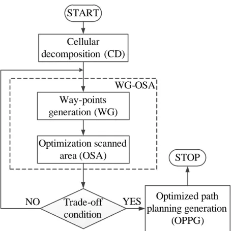
4.3.2 Proposed algorithm for infected areas detection . . . 64
4.3.2.1 Cellular Decomposition (CD) . . . 65
4.3.2.2 Way-points generation (WG) . . . 68
4.3.2.3 Optimization of the percentage of coverage (OSA) . . . 71
4.3.2.4 Optimized path planning generation . . . 72
4.4 Pesticide spraying . . . 77
4.4.1 Problem statement and decomposition . . . 77
ix
4.4.2 Map division (MD) . . . 79
4.4.2.1 Classification of infected areas . . . 79
4.4.2.2 Calculation of polygons for covering all the infected areas . 80 4.4.2.3 Minimal Convex Partitions . . . 80
4.4.3 Trajectory generation (TG) . . . 81
4.4.3.1 Waypoints generation for convex polygon . . . 82
4.4.3.2 Trajectory generation for each convex polygon . . . 83
4.4.3.3 Trajectory generation for entire agriculture area . . . 84
4.4.3.4 Simulation results . . . 85
4.5 Conclusion . . . 87
5 Nonlinear robust control and state estimation of UAVs 89 5.1 Control system for quadcopter . . . 91
5.2 Quadrotor’s states and parameters estimation . . . 93
5.2.1 State estimation overview . . . 93
5.2.2 Quadrotor’s parameters estimation . . . 93
5.2.3 Calculation/estimation of mass and moments of inertia . . . 94
5.3 Position/Altitude control . . . 95 5.3.1 Position control . . . 96 5.3.2 Altitude control . . . 97 5.4 LPV H∞ Attitude control . . . 98 5.4.1 Roll-pitch H∞ controller . . . 98 5.4.2 Yaw H∞ controller . . . 101
5.4.3 Simulation results and discussions . . . 102
5.4.4 Comments on the simulation results . . . 105
5.5 Attitude/Altitude Linear Parameter Varying (LPV) Unknown Input Observer (UIO) . . . 106
5.5.1 Problem formulation . . . 107
5.5.2 LPV UIO design for LPV system . . . 108
5.5.3 Convergence analysis and LMI formulation . . . 110
5.5.4 LPV UIO design . . . 112
5.5.4.1 LPV UIO for Roll-Pitch . . . 112
5.5.4.2 Linear Parameter Varying (LPV) Unknown Input Observer (UIO) for Yaw . . . 114
5.5.4.3 LPV UIO for Altitude . . . 115
5.5.5 Simulation results . . . 117
5.6 Attitude/Altitude LPV H∞ State feedback Controller . . . 120
5.6.1 System model and problem statement . . . 120
5.6.1.1 Quadrotor model . . . 120
5.6.1.2 Actuator model . . . 122
5.6.1.3 Simplified model . . . 122
5.6.2 Preliminary concepts . . . 126
5.6.3 LPV Attitude State feedback controller design . . . 127
5.6.4 Practical controller design . . . 128
5.6.5 Testing scenario . . . 130
5.6.6 Remarks on simulation results . . . 132
5.7.1 More simplified model . . . 132
5.7.2 Controller Design . . . 135
5.7.3 Practical controller design . . . 137
5.7.4 Testing scenario . . . 137
5.7.5 Comments on the simulation results . . . 138
5.8 Conclusion . . . 139
6 Simulation results 141 6.1 Coverage Path Planning (CPP) simulations . . . 142
6.1.1 Coverage Path Planning (CPP) for disease detection . . . 142
6.1.2 Coverage Path Planning (CPP) for crops spraying . . . 148
6.2 Quadrotor Control simulations . . . 153
6.2.1 Quadrotor stabilization . . . 153
6.2.1.1 Linear Parameter Varying (LPV) H∞state feedback controller153 6.2.2 Quadrotor Unknown Input Observer (UIO) . . . 158
6.2.2.1 Quadrotor Unknown Input Observer (UIO) without measure-ment noise . . . 158
6.2.2.2 Quadrotor Unknown Input Observer (UIO) with measure-ment noise . . . 165
6.2.3 Quadrotor path following . . . 172
6.3 Conclusion . . . 185
7 General conclusion and perspectives 187 7.1 Conclusions . . . 187
7.2 Perspectives . . . 188
A Preliminaries 191 A.0.1 Linear Parameter Varying (LPV) system . . . 191
A.0.2 Observability and Detectability of LPV systems . . . 200
A.0.3 Filtering the input . . . 201
A.0.4 Controller design for polytopic LPV systems . . . 201
B Clustering method 205
C Minimal convex polygon decomposition 207
D CGAL library 209
xi
List of Figures
1.1 Examples of mobile robots in PA . . . 3
2.1 Nano UAV robots . . . 15
2.2 Mini UAV robots . . . 16
2.3 Small UAV robots . . . 16
2.4 Medium UAV robots . . . 16
2.5 Laege UAV robots . . . 17
2.6 High-attitude long-endurance (HALE) UAV robots . . . 17
2.7 Medium-attitude long-endurance (HALE) UAV robots . . . 18
2.8 Medium-Range or tactile UAV (TUAV) robots . . . 18
2.9 Close-Range UAV . . . 18
2.10 Mini UAV robots . . . 18
2.11 Mini UAV robots . . . 19
2.12 Nano UAV robots . . . 19
2.13 Nano UAV robots . . . 19
2.14 Classification of drones’ applications[158] . . . 20
2.15 Multirotors classification according to the principle of flight . . . 24
2.16 Quadrotor configurations . . . 25
2.17 Regions of interest . . . 26
2.18 Simple geometric patterns for coverage path planing . . . 27
2.19 Exact cellular decomposition method and adjacency graph . . . 28
2.20 Exact cellular decomposition method . . . 29
2.21 Approximate cellular decomposition method . . . 30
3.1 Inertial Frame . . . 39
3.2 Vehicle-1 Frame . . . 39
3.3 Vehicle-2 Frame . . . 39
3.4 Body fixed Frame . . . 39
3.5 The Inertial Frame to Body frame . . . 40
3.6 Quadcopter configuration with coordinate frames and forces . . . 42
3.7 Roll motion . . . 43 3.8 Pitch motion . . . 43 3.9 Yaw motion . . . 43 3.10 Hovering motion . . . 43 3.11 Z motion . . . 44 3.12 Aerodynamic phenomena [32] . . . 46
4.1 Path planning by Probabilistic RoadMap (PRM) . . . 58
4.2 Path planning by RRT . . . 59
4.3 Coverage path planing problem formulation . . . 60
4.4 Coverage path planing problem formulation . . . 61
4.5 Augmentation of the size of obstacles . . . 61
4.6 UAV with frame picture capture . . . 63
4.7 Picture frames . . . 63
4.8 Proposed algorithm . . . 64
4.9 Cellular Decomposition (CD) methods . . . 66
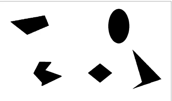
4.10 Agricultural area with convex and concave obstacles . . . 67
4.11 Critical points . . . 67
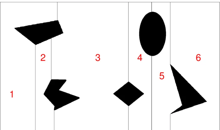
4.12 Cells after decomposition . . . 68
4.13 Picture frames . . . 69
4.14 Rectangles with centers in obstacles . . . 69
4.15 Picture frames that centers are not in obstacles . . . 70
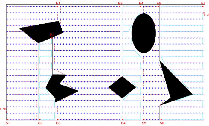
4.16 Boustrophedon path in each cell . . . 70
4.17 Cellular decomposition to cells . . . 71
4.18 In/Out points in each cell . . . 73
4.19 Travelling Salesman problems with additional constraints for this problem . 74 4.21 Genetic algorithm using in this approach . . . 74
4.20 Swap, flip, and slide operations for GA . . . 75
4.22 Cellular Decomposition (CD) in the proposed approach . . . 75
4.23 Genetic algorithm using in the proposed approach . . . 76
4.24 Problem definition . . . 78
4.25 Path planning Algorithm . . . 79
4.26 UAV with frame picture capture . . . 79
4.27 Division infected areas to several smaller regions . . . 80
4.28 Infected points covered by poygonal decompositions . . . 81
4.29 Minimal convex polygon decomposition . . . 81
4.30 Map division . . . 82
4.31 Trapezoid . . . 82
4.32 Way-points of trapezoid . . . 82
4.33 Augmentation of the size of obstacles . . . 83
4.34 Algorithm for way-point of infected area . . . 84
4.35 Waypoints generation for infected areas . . . 85
4.36 Simulation result . . . 86
5.1 Connection between rotational and translational subsystems of the quadcopter 92 5.2 General Controller system structure for quadcopter . . . 93
5.3 Moment of inertia of the systems quadcopter-mass . . . 94
5.4 Roll Pitch H∞ controller. . . 99
5.5 Yaw H∞ controller. . . 101
5.6 Variation of mass and moments of inertia and disturbances. . . 102
5.7 Translation coordinates: X, Y, Z. . . 103
5.8 Orientation coordinates: ϕ, θ, ψ. . . 103
5.9 Error in X, Y, Z, ψ. . . 104
xiii
5.11 Input signals: U1, U2, U3, U4. . . 105
5.12 Horizontal trajectory. . . 105
5.13 3D trajectory. . . 106
5.14 Unknown Input Observer for dynamic system . . . 110
5.15 Variations of mass and moments of inertia . . . 117
5.16 States z,ϕ,θ,ψ vs estimated states ˆz, ˆϕ, ˆθ, ˆψ . . . 118
5.17 States ˙z, ˙ϕ, ˙θ, ˙ψ vs estimated states ˙ˆz, ˙ˆϕ, ˙ˆθ, ˙ˆψ . . . 118
5.18 Unknown Inputs estimation . . . 119
5.19 States z,ϕ,θ,ψ vs estimated states ˆz, ˆϕ, ˆθ, ˆψ . . . 119
5.20 States ˙z, ˙ϕ, ˙θ, ˙ψ vs estimated states ˙ˆz, ˙ˆϕ, ˙ˆθ, ˙ˆψ . . . 119
5.21 Unknown Inputs estimation . . . 119
5.22 Quadcopter . . . 125
5.23 Control structure . . . 125
5.24 Block diagram of the attitude robust controller with augmented states and weight functions . . . 129
5.25 Variations of Mass, Ix, Iy, and Iz . . . 131
5.26 Impulse references ϕ, θ, ψ, impulse reference z, and impulse disturbances dϕ, dθ, dψ, dz . . . 131
5.27 Random references ϕ, θ, ψ, impulse reference z, and random disturbances dϕ, dθ, dψ, dz . . . 131
5.28 Sine references ϕ, θ, ψ, step reference z, and sine disturbances dϕ, dθ, dψ, dz 131 5.29 Measured and reference path . . . 136
5.30 Absolute error on path following . . . 136
5.31 Measured and reference value for the altitude . . . 136
5.32 Measured and reference values for the pitch angle . . . 136
5.33 Measured and reference values for the roll angle . . . 138
5.34 Measured and reference values for the yaw angle . . . 138
5.35 Measured and reference value for the altitude for added mass . . . 138
5.36 Measured and reference values for the pitch angle for added mass . . . 138
5.37 Measured and reference values for the roll angle for added mass . . . 139
5.38 Measured and reference value for the yaw angle for added mass . . . 139
6.1 Agricultural area with obstacles and infected points . . . 142
6.2 Scenario 1 Original images with obstacles used for infected area detection . . 143
6.3 Scenario 1: Infected area detection Critical points . . . 144
6.4 Scenario 1: Infected area detection Cellular decomposition . . . 144
6.5 Scenario 1: Infected area detection Image frames . . . 144
6.6 Scenario 1: Infected area detection Image frames in obstacles . . . 144
6.7 Scenario 1: Infected area detection Image frames in obstacles free . . . 145
6.8 Scenario 1: Infected area detection Boustrophedon path in cells . . . 145
6.9 Scenario 1: Infected area detection Start Stop Points in cells . . . 146
6.10 Scenario 1: IA detection paths for changing cells using PRM TSP . . . 146
6.11 Scenario 1: IA detection full path . . . 147
6.12 Scenario 2: Scenario 1 IA spraying obstacles and infected points . . . 148
6.13 Scenario 2: IA spraying minimal Divide infected areas to classes . . . 148
6.14 Scenario 2: IA spraying minimal convexy polygons vs obstacles . . . 149
6.16 Scenario 2: IA spraying obstacle free minimal convex polygons vs obstacles . 149
6.17 Scenario 2: IA spraying obstacle free boundary polygons vs obstacles . . . . 149
6.18 Scenario 2: IA spraying minimal convex decomposition . . . 150
6.19 Scenario 2: IA spraying boundary polygon . . . 150
6.20 Scenario 2: IA spraying minimal convex decomposition path . . . 150
6.21 Scenario 2: IA spraying boundary polygon path . . . 150
6.22 Scenario 2: IA spraying minimal convex decomposition START STOP points 151 6.23 Scenario 2: IA spraying boundary decomposition START STOP points . . . 151
6.24 Scenario 2: IA spraying paths for changing cells using prm tsp . . . 151
6.25 LPV H∞Altitude/Attitude State Feedback Controller for mass-varying quad-copter configuration . . . 153
6.26 Scenario 3: Mass, Ix, Iy, and Iz LPV H∞ Alt/Att State Feedback Controller 154 6.27 Scenario 3: U1, U2, U3, and U4 LPV H∞ Alt/Att State Feedback Controller 154 6.28 Scenario 3: ϕ, θ, ψ, and z LPV H∞ Alt/Att State Feedback Controller . . . 155
6.29 Scenario 3: eϕ, eθ, eψ, and ez LPV H∞ Alt/Att State Feedback Controller . 155 6.30 Scenario 4: Mass, Ix, Iy, and Iz LPV H∞ Alt/Att State Feedback Controller 156 6.31 Scenario 4: U1, U2, U3, and U4 LPV H∞ Alt/Att State Feedback Controller 156 6.32 Scenario 4: ϕ, θ, ψ, and z LPV H∞ Alt/Att State Feedback Controller . . . 157
6.33 Scenario 4: eϕ, eθ, eψ, and ez LPV H∞ Alt/Att State Feedback Controller . 157 6.34 LPV H∞ UIO for mass-varying quadcopter configuration . . . 158
6.35 Scenario 5: Mass, Ix, Iy, and Iz LPV UIO for Alt/Att . . . 159
6.36 Scenario 5: UI and their estimation with LPV UIO for Alt/Att . . . 160
6.37 Scenario 5: UI estimations errors with LPV UIO for Alt/Att . . . 160
6.38 Scenario 5: Z, φ, θ, and ψ and estimations LPV UIO for Alt/Att . . . 160
6.39 Scenario 5: Differences between (real and estimated) vs (real and measured) values LPV UIO for Alt/Att . . . 160
6.40 Scenario 5: ˙Z, ˙φ, ˙θ, and ˙ψ and estimations LPV UIO for Alt/Att . . . 161
6.41 Scenario 5: Differences between (real and estimated) vs (real and measured) values LPV UIO for Alt/Att . . . 161
6.42 Scenario 6: Mass, Ix, Iy, and Iz LPV UIO for Alt/Att . . . 162
6.43 Scenario 6: UI and their estimation with LPV UIO for Alt/Att . . . 163
6.44 Scenario 6: UI estimations errors with LPV UIO for Alt/Att . . . 163
6.45 Scenario 6: Z, φ, θ, and ψ and estimations LPV UIO for Alt/Att . . . 163
6.46 Scenario 6: Differences between (real and estimated) vs (real and measured) values LPV UIO for Alt/Att . . . 163
6.47 Scenario 6: ˙Z, ˙φ, ˙θ, and ˙ψ and estimations LPV UIO for Alt/Att . . . 164
6.48 Scenario 6: Differences between (real and estimated) vs (real and measured) values LPV UIO for Alt/Att . . . 164
6.49 LPV H∞ UIO for mass-varying quadcopter configuration . . . 165
6.50 Scenario 7: Mass, Ix, Iy, and Iz LPV UIO for Alt/Att . . . 166
6.51 Scenario 7: UI and their estimation with LPV UIO for Alt/Att . . . 167
6.52 Scenario 7: UI estimations errors with LPV UIO for Alt/Att . . . 167
6.53 Scenario 7: Z, φ, θ, and ψ and estimations LPV UIO for Alt/Att . . . 167
6.54 Scenario 7: Differences between (real and estimated) vs (real and measured) values LPV UIO for Alt/Att . . . 167
xv 6.56 Scenario 7: Differences between (real and estimated) vs (real and measured)
values LPV UIO for Alt/Att . . . 168
6.57 Scenario 8: Mass, Ix, Iy, and Iz LPV UIO for Alt/Att . . . 169
6.58 Scenario 8: UIO Moments estimations LPV UIO for Alt/Att . . . 170
6.59 Scenario 8: UIO Moments estimations errors LPV UIO for Alt/Att . . . 170
6.60 Scenario 8: Z, φ, θ, and ψ and estimations LPV UIO for Alt/Att . . . 170
6.61 Scenario 8: Differences between (real and estimated) vs (real and measured) values LPV UIO for Alt/Att . . . 170
6.62 Scenario 8: ˙Z, ˙φ, ˙θ, and ˙ψ and estimations LPV UIO for Alt/Att . . . 171
6.63 Scenario 8: Differences between (real and estimated) vs (real and measured) values LPV UIO for Alt/Att . . . 171
6.64 LPV H∞ UIO for mass-varying quadcopter configuration . . . 172
6.65 Scenario 9: Mass, Ix, Iy, and Iz Quadrotor path following . . . 174
6.66 Scenario 9: x, y, and z, their responses, and disturbances Quadrotor path following . . . 174
6.67 Scenario 9: U1, U2, U3 and U4 Quadrotor path following . . . 174
6.68 Scenario 9: Errors on X, Y , Z and ψ Quadrotor path following . . . 174
6.69 Scenario 9: X and Y in 2D Quadrotor path following . . . 175
6.70 Scenario 9: X, Y , and Z in 3D Quadrotor path following . . . 175
6.71 Scenario 9: X, Y , and Z vs time Quadrotor path following . . . 175
6.72 Scenario 10: Mass, Ix, Iy, and Iz Quadrotor path following . . . 177
6.73 Scenario 10: x, y, and z, their responses, and disturbances Quadrotor path following . . . 177
6.74 Scenario 10: U1, U2, U3 and U4 Quadrotor path following . . . 177
6.75 Scenario 10: Errors on X, Y , Z and ψ Quadrotor path following . . . 177
6.76 Scenario 10: X and Y in 2D Quadrotor path following . . . 178
6.77 Scenario 10: X, Y , and Z in 3D Quadrotor path following . . . 178
6.78 Scenario 10: X, Y , and Z vs time Quadrotor path following . . . 178
6.79 Scenario 11: Mass, Ix, Iy, and Iz Quadrotor path following . . . 180
6.80 Scenario 11: x, y, and z, their responses, and disturbances Quadrotor path following . . . 180
6.81 Scenario 11: U1, U2, U3 and U4 Quadrotor path following . . . 180
6.82 Scenario 11: Errors on X, Y , Z and ψ Quadrotor path following . . . 180
6.83 Scenario 11: X and Y in 2D Quadrotor path following . . . 181
6.84 Scenario 11: X, Y , and Z in 3D Quadrotor path following . . . 181
6.85 Scenario 11: X, Y , and Z vs time Quadrotor path following . . . 181
6.86 Scenario 12: Mass, Ix, Iy, and Iz Quadrotor path following . . . 183
6.87 Scenario 12: x, y, and z, their responses, and disturbances Quadrotor path following . . . 183
6.88 Scenario 12: U1, U2, U3 and U4 Quadrotor path following . . . 183
6.89 Scenario 12: Errors on X, Y , Z and ψ Quadrotor path following . . . 183
6.90 Scenario 12: X and Y in 2D Quadrotor path following . . . 184
6.91 Scenario 12: X, Y , and Z in 3D Quadrotor path following . . . 184
xvii
List of Tables
1.1 The use of autonomous robot in PA . . . 6
4.1 Some results for simulations in Matlab . . . 72
4.2 Some results for simulations in Matlab . . . 72
4.3 Time of simulation . . . 74
4.4 Minimal convex polygon vs Boundary polygon . . . 85
4.5 Classes number vs Trajectory path length . . . 87
5.1 Parameters range for LPV H∞ Roll-Pitch and Yaw controllers . . . 100
5.2 Quadcopter parameters definition . . . 117
5.3 Variation ranges of varying parameters . . . 118
5.4 Quadcopter parameters definition . . . 130
xix
List of Abbreviations
LMI Linear Matrix Inequality LPV Linear Parameter Varying UAV Unmanned Aerial Vehicle IMU Inertial Measurement Unit CoG Center of Gravity
DOF Degrees of Freedom
GPS Global Positioning System
DGPS Differential Global Positioning System VTOL Vertical Take-Off and Landing
CT LPV Continuous Time Linear Parameter Varying DT LPV Discrete Time Linear Parameter Varying LTI Linear Time Invariant
UIO Unknown Input Observer PA Precision Agriculture IoT Internet of Things
ICT Information and Communication Technology CPP Coverage Path Planning
TSP Travelling Salesman Problem GA Genetic Algorithm
PID Proportional Integral Derivative PI Proportional Integral
PD Proportional Derivative DOB Disturbance Observer Based LQR Linear Quadratic Regulator
LQG Linear Quadratic Gaussian SMC Sliding Mode Control STA Super Twisting Algorithm MPC Model Predictive Control
RRT Rapidly-exploring Random Tree PRM Probabilistic RoadMap
CD Cellular Decomposition TS Takagi-Sugeno
KF Kalman Filter
EKF Extended Kalman Filter DCM Direction Cosine Matrix OKF Optimal Kalman Filter
xxi
List of Symbols
N The set of natural numbers
Z The set of integers
R The set of real numbers
R+ The set of non-negative real numbers
R>0 The set of positive real numbers
Rn n-dimensional vector space over the field of the real numbers eig(A) The set of eigenvalues of square matrix A ∈ Rn×n
sec(x) The secant function cos x1
Positive definite symbol ≺ Negative definite symbol
1
1
Introduction
This chapter briefly introduces the needs of using robots, especially Unmanned Aerial Vehicle (UAV) in Precision Agriculture (PA) for increasing crop yields. Firstly, sustain-able food production challenges are given in section 1.1. Then, the definition of PA is introduced in section 1.2. The uses of the mobile robot and UAV in PA are studied respectively in subsections 1.3 and 1.4. Our motivations and the objectives of the thesis are highlighted in section 1.5 and 1.6 respectively. The main contributions are listed in sections 1.7. Finally, the structure of the thesis document is outlined in section 1.8.
Chapter abstract
This Chapter contains:
1.1 Sustainable food production . . . 2 1.2 Precision Agriculture (PA) . . . 2 1.3 The use of mobile robot in PA . . . 3 1.4 The use of UAV in PA . . . 4 1.4.1 Monitoring . . . 4 1.4.2 Weed mapping and management . . . 4 1.4.3 Crop spraying . . . 5 1.4.4 Irrigation management . . . 5 1.4.5 Vegetation growth monitoring and yield estimation . . . 6 1.5 Motivations . . . 7 1.6 Objectives . . . 7 1.7 Contribution of the thesis . . . 8 1.8 Structure of the thesis . . . 9 1.9 Publications . . . 10
1.1
Sustainable food production
According to the Food and Agriculture Organization (FAO, 2009a), it is estimated that by 2050 the world’s population will reach 9 billion and this population change mainly occurs in developing countries [68]. Consequently, ensuring a sustainable supply of food for the world’s fast-growing population is a major challenge. Added to the challenge is that sustainable food products need to be nutrient-dense to allow people to have a diverse diet that contains a balanced and adequate combination of energy and nutrients to support good health [240]. Sustainable food production is "a method of production using processes and systems that are non-polluting, conserve non-renewable energy and natural resources, are economically efficient, are safe for workers, communities and consumers, and do not compromise the needs of future generations"[76].
Although the area of land for agriculture is declining, water resources for cultivation are in-creasingly scarce, climate change [169], global warming [178], more pests appear, more food still have to be produced. These negative effects on agriculture can be offset to some degree by improving pest control technologies, implementing crop rotations, soil and water conser-vation, altering crop varieties, employing other sound ecological technologies for resource use in agriculture, and machinery applications in agricultural production.
1.2
Precision Agriculture (PA)
Precision Agriculture (PA) can be defined as "the application of modern information tech-nologies to provide, process and analyze multi source data of high spatial and temporal resolution for decision making and operations in the management of crop production"[47]. The main goal of PA is the process of gathering, processing, and analyzing temporal, spa-tial, and individual data to support management decision making. This decision greatly affects improved resource use efficiency, productivity, quality, profitability and sustainability of agricultural production
Autonomous robots can be applied in a variety of field operations of PA. The use of Au-tonomous robots facilitate the processes of capturing and processing high quantities of data. They also provide the required capabilities for operating not only at the individual plant level but also at the complete field level. In [26], authors propose autonomous platforms which can be used for cultivation and seeding, weeding, scouting, application of fertilizers, irrigation, and harvesting.
For the reason that economic benefits should be easily achieved without requiring the in-tegration of additional components or decision support systems, several advanced robotic technologies have been widely applied in PA such as autonomous guidance, autosteer, re-mote sensing, and controls.
The most important abilities of automatic agricultural robots can be categorized into four categories [40]:
• Guidance: the robot has to self-locate its position in the agricultural environment. • Detection: the robot should have the ability to detect the biological features from the
1.3. The use of mobile robot in PA 3 • Action: Based on the information on the first two categories, the robot should execute the task for which the vehicle was designed, such as spraying, monitoring, or harvesting. • Mapping: the robot could construct the map of the agricultural field.
For accomplishing all the previously mentioned activities, the devices (sensors) such as Real-Time Kinetics Global Positioning System (RTK-GPS), camera, and Light Detection and Ranging (LiDAR) have to retrieve information from the environment and send them to the processing unit of the robot. This information can be the states of the robot(location, velocity,...) or the information related to the agriculture area. Then, a decision will be made based on the gathered information to accomplish the predefined tasks.
There are several types of agriculture robots. However, they can be defined as two main groups: mobile robot and aerial robot. In the next two subsections, the use of mobile robot and aerial robot in PA will be considered.
1.3
The use of mobile robot in PA
Mobile robots (Fig. 1.1) have been widely used in precision agriculture to reduce human labor and increase productivity. Farmers can use the tractors, harvesters, and they are self-guided by GPS, Robots can automate operations like pruning, thinning, mowing, spraying, and weed removal, Sensor technology is used to manage the pests and diseases that affect crops. Some
(a) Hortibot robot[105]
source: www.technologyreview.com
(b) Kongskilde Robotti robot[88]
source: conpleks.com
Figure 1.1: Examples of mobile robots in PA
examples of the application of mobile robot are autonomous targeted spraying for pest control in commercial greenhouses [176], to optimum manipulator design for autonomous de-leafing process of cucumber plants [95], simultaneous localization and mapping techniques for plant trimming [34], automated harvesting of valuable fruits (for example on sweet pepper[184][94], oil palm [206], mango [209], cucumber [229], almond [227], apple [161][101], strawberry [91], cherry fruit [215], citrus [147], vineyard [246], and tomato [182][181][233]).
Besides mobile robots, flying robots are also widely used in PA. The applications of UAVs will be introduced in the next subsection.
1.4
The use of UAV in PA
The combination of modern technologies such as the Internet of Things (IoT), Information and Communication Technology (ICT), control theory, image processing, and especially the accelerated development of the UAV technology provides a promising solution to PA [212] to deal with the challenges of food sustenation problem. UAVs have been widely used in many applications of PA such as monitoring, weed mapping and management, crop spraying, etc. The specific applications of UAV in PA will be covered in this subsection.
1.4.1
Monitoring
A very common application of PA is to determine the crop health situation by using Remote Sensing (RS) techniques and image analysis. Images can be captured by satellites [22][156]or UAVs [18][144]. However, satellite images are not good choice due to the low spatial resolu-tion of acquired images, restricresolu-tions of the temporal resoluresolu-tions as satellites are not always available to capture the necessary images, the quality of the images depends on the weather condition and camera costs. Another method that gives better quality of the images is using the manned aircraft. Though, this method is still costly.
Crops health is a very important factor that determines the quality and quantity of the crop. Therefore, the crops health and diseases detection must be monitored [51][185][155][116] continuously to detect disease promptly and avoid spreading problems. Normally, crop health is often monitored by agricultural experts. Nevertheless, this is a very time-consuming task, as it requires several weeks or even months for inspecting an entire crop and preventing the potentials of “continuous” disease spreading. Another method that can be applied to prevent crop disease is to spray pesticides at fixed times during the plant’s growth. This method has been applied and is relatively popular in developed countries, however, it is high cost and also increases the likelihood of groundwater contamination as pesticide residues in the products and soil.
The applicable of UAV in PA for monitoring the crop’s health conditions provide excellent possibilities to obtain field data in an easy, fast, efficient, and cost-effective way compared to the aforementioned methods. UAVs equipped with specialized cameras are used for gathering photos of the entire plant area. The changes in plant biomass and their health can be determined by using special algorithms for analyzing the crop imaging information. Thus, diseases can be determined in their early stages enabling farmers to intervene in order to reduce losses. For this purpose,UAVs can be used in the two different stages of disease control as: (i) UAVs are used to collect crop images. Analyze the gathered images for detecting a possible infection before visual indications appear. Map infected areas for treatment; and (ii) during the treatment of infection, the UAV is used to spray insecticides to precisely the locations of the infected plants that were mapped in the previous period.
1.4.2
Weed mapping and management
Another application of UAV in PA is weed mapping [99][174][98][200][19]. Weeds are non-desirable crops, they grow simultaneously with the crop in agricultural areas and cause a number of serious problems. They use the same resources such as soil, water, nutrients, and space on agricultural land as crops and affect crop growth. Traditionally, herbicides
1.4. The use of UAV in PA 5 are used for controlling the weeds. The same amounts of herbicides are sprayed over the entire field, even within the weed-free areas. Such a strategy incurs a waste of herbicides, potentially contaminating soil resources. Moreover, overuse of herbicides can lead to the evolution of herbicide-resistant weeds and it can affect crop growth and productivity. To overcome the above problems the agriculture area is divided into zones that each one receives customized management because as usual weeds spread through only a few spots of the field. Consequently, it is necessary to generate an accurate weed cover map for precise spraying of herbicide. UAVs are used to gathering images. Then, the gathered images are analyzed to generate a precise weed cover map depicting the spots where the chemicals are needed and the needed amount of herbicide for each spot.
1.4.3
Crop spraying
The traditional spraying equipment used in conventional farming is the manual air-pressure or battery-powered knapsack sprayers. However, this traditional spraying equipment causes a non-minor loss of pesticides due to the mechanical structure of the injector and the spraying is done manually. Furthermore, the operators have to be present when spraying, resulting in contact with operators and possibly affecting human health.
Therefore, the use of UAVs to spray pesticides [217][235][69][81][244] can reduce the opera-tor’s exposure to chemicals, reduce pesticide losses, and save time. An uncrewed helicopter, which is equipped with small pesticide tanks, was developed and introduced in Japan in the 1980s [212] for crop spraying. By analyzing image data, we can determine exactly and pest status of the crop on the whole area of agriculture. Because the level of plant pests and diseases varies from region to region, the amount of insecticide to be sprayed must also be different to ensure uniform plant growth. Path planning algorithms based on crop data not only create the optimal motion trajectory for the UAV, but also optimize the amount of needed agrochemical products.
1.4.4
Irrigation management
Currently, the process of irrigation for crops consumes about 70% of the water in the world. [38][196], while water resources are increasingly exhausted. Therefore, crop irrigation man-agement [190][12][168][183] is a very important task in PA. Precision irrigation techniques must be improved and monitored more strictly to lead to the more efficient use of water: (i) in the right place; (ii) at the right time; and (iii) in correct quantities.
Typically, water is evenly irrigated over the entire crop area, although the amount of water actually needed for different areas varies. Therefore, determining the appropriate amount of water to irrigate in different areas can help farmers save time and water resources. Moreover, such precise farming techniques can lead to increased yields and crop quality. Dividing agricultural land into different irrigation areas, for precise management of resources, can be done easily by using UAV. Special sensors equipped on the UAVs give them the ability to classify and identify areas where plants need more water. Besides, based on data collected from UAV, we can create specialized maps that illustrate the morphology of the soil for more efficient irrigation, suitable for each type of crop and each specific area.
Table 1.1: The use of autonomous robot in PA
Publication Robot type Operation Technique [180] Aerial robot Monitoring Process
- Monitoring vege-tation state
Multispectral camera, GPS sys-tem, FlightCTRL, NaviCtTRL, First person view platform, GSM modem, Magnetic compass
[13] Aerial robot Monitoring Process -Detecting drainage pipes
VIS Camera, NIR Camera, Ther-mal Camera
[110] Aerial robot Monitoring Pro-cess -Evaluating water stress and vegetation state
Thermal camera, Multispectral camera, Single-board computer, GPS system, Stabilization mech-anism
[249] Aerial robot Monitoring Process - Estimating nitro-gen state
Hyperspectral camera [49] Aerial robot Spraying Process
-Spraying fruits and trees
Spraying Device, Multispectral camera, IMU, Magnetometer. Barometer, Servos
[193] Aerial robot Investigating com-putational
resources during a monitoring process
IMU, GPS system
[198] Aerial robot Evaluating water
stress FlightCtrl, NaviCtrl, 3-axis ac-celerometer, Thermal Camera, Storing device, Pressure sensor, Digital compass, GPS system [228] Mobile
robot Coverage path plan-ning Harmony Search (HS) algorithmfor finding complex coverage tra-jectories
[192] Mobile
robot Field mapping 3D terrain maps, stereo camera,location sensor, IMU [199] Mobile
robot Weed and pest con-trol Image processing, decision controlalgorithms [217] Mobile
robot Weeding Automatic computer vision, dif-ferential spraying to control the weeds.
1.4.5
Vegetation growth monitoring and yield estimation
UAVs are also often applied in monitoring vegetation growth and providing estimates of productivity [250][230][106][92]. One of the main major difficulties of increasing agricultural
1.5. Motivations 7 productivity and quality is the lack of means to systematically monitor the process of cul-tivation. Therefore, collecting and analyzing information related to crop growth regularly using the UAV provide an increased opportunity to track crop growth and observe changes in some parameters of the field.
Many works have been focusing on observing the biomass and nitrogen status of crops besides the yield estimation. Biomass of crops and nitrogen content status are the main parameters to determine the need for additional fertilizer or other actions. Furthermore, various parameters, such as crop height, the distance between rows or between plants, and the index Leaf Area Index (LAI) can be estimated by using the three-dimensional digital maps of the crop which is created by the gathered images by the UAVs. By analyzing the information gathered about crops by UAVs, farmers can make plans to control crop management, decide when to irrigate, spray pesticides, or harvest.
Table 1.1 provides examples of the developments of autonomous mobile and aerial robots in PA.
1.5
Motivations
We are motivated, in this thesis, by the coverage path planning scenario and control of Un-manned Aerial Vehicle (UAV) in Precision Agriculture (PA) for the two tasks, crop inspection and crop spraying.
Although the application of Unmanned Aerial Vehicle (UAV) in Precision Agriculture (PA) has been being studied intensively, however, many challenges are still open with respect to the coverage path planning scenarios as the requirements to visit all the predefined points while avoiding obstacles and minimize some objective functions.
In the control aspect, the UAV has to follow as most accurately as possible according to the given trajectory under the influence of disturbances such as wind or changes of dynamic parameters such as mass or moments of inertia during flying time.
1.6
Objectives
The objective of this thesis is to realize the modeling, planning, and control of an unmanned helicopter robot for monitoring large areas, especially in PA applications. Several tasks in PA are addressed such as monitoring, insecticides spraying.
• Path planning objective: In pest surveillance missions, drones will be equipped with specialized cameras. In order to monitor the whole agriculture area, we need to capture images by specialized cameras. A trajectory will be researched and generated to enable the UAV to capture images of entire crop areas and avoid obstacles during flight. Infected areas will be then identified by analyzing gathered images.
• Control objective: In insecticides spraying, the UAV must be controlled to fly in a pre-programmed trajectory, which has been generated in the path planing task, and spray the insecticide over all the infected crop areas. The UAV is equipped with pesticide tank and a mechanical or hydraulic system for pesticide spraying. During the spraying of insecticides, the mass of UAV will decrease over time, resulting in changes
in the dynamic parameters of UAV such as the moments of inertia. In addition, during the mission, UAV is affected by disturbances such as wind gusts. The changes in the kinetic parameters and the external disturbances cause instability of the UAV. Consequently, a robust controller has to be designed to stabilize the UAV and to follow exactly the predefined trajectory while keep stabilizing the UAV under the changes in the kinetic parameters and the external disturbances.
1.7
Contribution of the thesis
The objective of this thesis is to realize the modeling, planning, and control of an unmanned UAV robot for monitoring large areas, especially in PA1applications. Several tasks in PA are
addressed. In pest surveillance missions, drones will be equipped with specialized cameras. A trajectory will be researched and created to enable unmanned aircraft to capture images of entire crop areas and avoid obstacles during flight. Infected areas will be then identified by analyzing taken images. In insecticides spraying, the aircraft must be controlled to fly in a pre-programmed trajectory and spray the insecticide over all the infected crop areas. In the first part, we present a new complete coverage path planning algorithm by proposing a new cellular decomposition which is based on a generalization of the Boustrophedon variant, using Morse functions, with an extension of the representation of the critical points. This extension leads to a decrease in the number of cells after decomposition. GA2 and TSP3
algorithm are then applied to obtain the shortest path for complete coverage. Next, from the information on the map regarding the coordinates of the obstacles, non-infected areas, and infected areas, the infected areas are divided into several non-overlapping regions by using a clustering technique. Then an algorithm is proposed for generating the best path for a UAV to distribute medicine to all the infected areas of an agriculture environment which contains non-convex obstacles, pest-free areas, and pests-ridden areas.
In the second part, we study the design of a robust control system that allows the vehicle to track the predefined trajectory for a dynamic model-changing UAV due to the changes of dynamic coefficients such as the mass and moments of inertia. Therefore, the robust observer and control laws are required to adopt the changes in dynamic parameters as well as the impact of external forces. The proposed approach is to explore the modeling techniques, planning, and control by the LPV type technique. To have easily implantable algorithms and adaptable to changes in parameters and conditions of use, we favor the synthesis of LPV4
UIO5, LPV quadratic state feedback, dynamic ouptut feedback, and static output feedback
controllers. The observers and controllers are designed by solving a set of Linear Matrix Inequality (LMI) obtained from the Bounded Real Lemma and LMI region characterization. Finally, to highlight the performance of the path planning algorithms and generated control laws, we perform a series of simulations in MATLAB Simulink environment. Simulation re-sults are quite promising. The coverage path planning algorithm suggests that the generated trajectory shortens the flight distance of the aircraft but still avoids obstacles and covers the
1Precision Agriculture (PA) 2Genetic Algorithm (GA)
3Travelling Salesman Problem (TSP) 4Linear Parameter Varying (LPV) 5Unknown Input Observer (UIO)
1.8. Structure of the thesis 9 entire area of interest. Simulations for the LPV UIO and LPV controllers are conducted with the cases that the mass and moments of inertia change abruptly and slowly. The LPV UIO is able to estimate state variables and the unknown disturbances and the estimated values converge to the true values of the state variables and the unknown disturbances in a short time. The LPV controllers work well for various reference signals (impulse, random, constant, and sine) and several types of disturbances (impulse, random, constant, and sine).
1.8
Structure of the thesis
The manuscript of the thesis is divided into 7 chapters:
• Chapter 1 - Introduction: Introduces the applications and necessity of robots, especially UAVs in PA. Moreover, it highlights our motivations, the specific challenges, objectives, and the main contributions of the thesis.
• Chapter 2 - State of the art: offers a short state of the art for UAVs and more par-ticularly the multirotors as typical vehicle for coverage path planning mission. Then, it also reviews the state of the art of the coverage path planning algorithms and control laws for quadcopters.
• Chapter 3 - System modeling: introduces the mathematical differential equations of quadcopter dynamics.
• Chapter 4 - Robust path planning: proposes a new approach for maximizing the coverage path planning while minimizing the path length of an aerial robot in agriculture environment with concave obstacles. For resolving this problem, we propose a new cellular decomposition which is based on a generalization of the Boustrophedon variant, using Morse functions, with an extension of the representation of the critical points. This extension leads to a decrease of the number of cells after decomposition. The results show that this new cellular decomposition works well even with several concave obstacles inside the environment. Furthermore, for path planning, the cells are divided again into two classes, leading to have a cell set better suited for use of the TSP to get complete coverage. GA and TSP algorithm are applied to obtain the shortest path. Then, an approach is also proposed to maximize the scanned area on the working area with obstacles. Then, we focus on generating the best path for an UAV to distribute medicine to all the infected areas of an agriculture environment which contains non-convex obstacles, pest-free areas and pests-ridden areas. The algorithm for generating this trajectory can save the working time and the amount of medicine to be distributed to the whole agriculture infected areas.
From the information on the map regarding the coordinates of the obstacles, infected areas, and infected areas, the infected areas are divided into several non-overlapping regions by using a clustering technique. There is a trade-off between the number of classes generated and the area of all the pests-ridden areas. After that, a polygon will be found to cover each of these infected regions. However, obstacles may occupy part of the area of these polygons that have been created previously. Each polygon that is occupied in part by obstacles can be further divided into a minimum number of obstacle-free convex polygons. Then, an optimal path length of boustrophedon trajectory will be created for each convex polygon that has been
created for the UAV to follow. Finally, this chapter deals with the process of creating a minimal path for the UAV to move between all the constructed convex polygons and generation of the final trajectory for the UAV which ensures that all the infected agriculture areas will be covered by the medicine.
• Chapter 5 - Control: During the spraying of insecticides, the mass of UAV will decrease over time, resulting in changes in the dynamic parameters of UAV such as the moments of inertia. In addition, during the mission, UAV is affected by disturbances such as wind. The changes in the kinetic parameters and the external disturbances cause instability of the UAV. Therefore, several robust control laws for quadcopter under disturbances and changes of the dynamic parameters have been developed such as LPV dynamic output feedback controller, LPV static output feedback controller, and LPV state feedback controller. We also design a Linear Parameter Varying (LPV) Unknown Input Observer (UIO) for quadcopters.
• Chapter 6 - Simulation and experiments: The simulations are conducted for both path planning and control tasks. This chapter also gives some comments on the simulation results and will discuss the advantages and performances of the proposed approaches.
• Chapter 7 - Conclusion and perspectives: Gives some concluding remarks as well as perspectives.
1.9
Publications
This work results in several publications in international conferences proceedings. Journal papers are submitted and are under review.
Published:
• T. H. Pham, Y. Bestaoui and S. Mammar, "Aerial robot coverage path planning ap-proach with concave obstacles in precision agriculture," 2017 Workshop on Research, Education and Development of Unmanned Aerial Systems (RED-UAS), Linkoping, 2017, pp. 43-48, doi: 10.1109/RED-UAS.2017.8101641.
• T. H. Pham and S. Mammar, "Quadrotor LPV Control using Static Output Feed-back," 2019 IEEE 16th International Conference on Networking, Sensing and Control (ICNSC), Banff, AB, Canada, 2019, pp. 74-79, doi: 10.1109/ICNSC.2019.8743181. • T. H. Pham, D. Ichalal, S. Mammar (2019). "LPV and Nonlinear-based control of
an Autonomous Quadcopter under variations of mass and moment of inertia". IFAC-PapersOnLine, 52(28), pp. 176 – 183. doi:10.1016/j.ifacol.2019.12.371.
• T. H. Pham, D. Ichalal, S. Mammar (2020). , "LPV state-feedback controller for Attitude/Altitude stabilization of a mass-varying quadcopter," 2020 20th International Conference on Control, Automation and Systems (ICCAS), Busan, Korea (South), 2020, pp. 212-218, doi: 10.23919/ICCAS50221.2020.9268310.
1.9. Publications 11 • T. H. Pham, D. Ichalal, S. Mammar (2020). "Complete coverage path planning for pests-ridden in precision agriculture using UAV," 2020 IEEE International Conference on Networking, Sensing and Control (ICNSC), Nanjing, China, 2020, pp. 1-6, doi: 10.1109/ICNSC48988.2020.9238122.
• T. H. Pham, D. Ichalal, S. Mammar (2020). "LPV Unknown Input Observer for Attitude of a mass-varying quadcopter". 16th International Conference on Control, Automation, Robotics and Vision, ICARCV 2020, Shenzhen, China, December 13 -15, 2020, pp. 917 – 924.
To be submitted:
• T. H. Pham, D. Ichalal, S. Mammar. "Discrete LPV state feedback preview control design for Attitude/Altitude of a mass-varying quadcopter".
• T. H. Pham, D. Ichalal, S. Mammar. "Attitude/Altitude LPV UIO-based controller design of a mass-varying quadcopter".
• T. H. Pham, D. Ichalal, S. Mammar. "Complete coverage path planning using UAV applied in precision agriculture under the consideration of dynamic constraints.
13
2
State of the art
This chapter offers a brief state of the art of Unmanned Aerial Vehicle (UAV). Firstly, a short review of UAV such as UAV classification, applications, advantages, and dis-advantages of UAV will be given in Section 2.1.1. Due to their special characteristics, which allow their use in a wide range of applications, we focus on particular Vertical Take-Off and Landing (VTOL) types of UAVs and especially the quadrotor configura-tion in Secconfigura-tion 2.2. Then the state of the arts of complete coverage of UAV and control of quadrotors are given in Section 2.3 and 2.4 respectively.
Chapter abstract
This Chapter contains:
2.1 Unmanned Aerial Vehicles . . . 15 2.1.1 Overview of unmanned aerial vehicles . . . 15 2.1.2 UAVs classification . . . 15 2.1.3 Applications of UAVs . . . 20 2.1.4 Advantage, disadvantages, and typical uses of UAVs . . . 21 2.1.4.1 Fixed Wing UAV . . . 21 2.1.4.2 Single Rotor UAV . . . 22 2.1.4.3 Multirotors UAVs . . . 22 2.2 Quadrotors . . . 23 2.3 Coverage Path planning methods used for UAV . . . 25 2.3.1 No Decomposition . . . 27 2.3.2 Cellular Decomposition (CD) . . . 28 2.4 State of the art on the control of quadcopters . . . 30 2.4.1 Proportional Integral Derivative controller . . . 31 2.4.2 Linear Quadratic Regulator (LQR)/Gaussian-LQR/G . . . 31 2.4.3 Sliding Mode Control (SMC) . . . 32 2.4.4 Backstepping Control . . . 32 2.4.5 Adaptive Control Algorithms . . . 33 2.4.6 Robust Control Algorithms . . . 33 2.4.7 Optimal Control Algorithms . . . 33 2.4.8 Model Predictive Control (MPC) . . . 34
2.4.9 Exact Feedback Linearization . . . 34 2.5 Conclusion . . . 35
2.1. Unmanned Aerial Vehicles 15
2.1
Unmanned Aerial Vehicles
2.1.1
Overview of unmanned aerial vehicles
An Unmanned Aerial Vehicle (UAV) or drone is an aircraft without passenger or pilot on-board which can fly autonomously based on pre-programmed flight plans, through the help of complex dynamic automation systems, or be controlled remotely by a pilot at a ground control station. Depending on its mission, endurance, and size, each UAV can carry different payloads.
UAVs are equipped with multiple sensors (such as Global Positioning System (GPS), Inertial Measurement Unit (IMU), Differential Global Positioning System (DGPS), accelerometer, magnetometer, pito tube, etc) and are connected in real time to many other systems at the ground control station. This allows the UAV to gain important information such as speed, position, heading, altitude, movement direction, temperature, speed and wind direction, the amount of fuel or remaining energy to perform the task, etc. UAV can perform a variety of tasks in military, civilian, and entertainment applications. Moreover, since they are free of screw on board, they can be designed to be smaller, can perform tasks that require greater flexibility, and can carry more payloads.
2.1.2
UAVs classification
There are many characteristics for classifying UAVs [107][138] based on their variety intended use.
Classification according to size
• Very small UAVs: are the unmanned aircraft with dimensions ranging from the size of a large insect to 30[cm]−50[cm] long. The very small UAVs can be sub-divided into
– Micro or nano UAVs: insect size is up to 15[cm].
– Mini UAVs: insect size is between 15[cm] and 50[cm].
The representative of very small UAVs is insect-like UAVs. Their popular micro design always has flapping or rotary wings. They are extremely small in size, very lightweight, and can be used for spying and biological warfare. Some of nano UAVs are shown in Fig. 2.12 Examples of mini UAVs are Xbird 250 quadro, Parrot bebop, Parrot Disco,
(a) Black Hornet (b) Hummingbird (c) Hummingbird (d) Dragonfly robot
Figure 2.1: Nano UAV robots
(a) Xbird 250 quadro (b) Parrot bebop (c) Parrot Disco (d)
Eagle VTOL Mapping
Figure 2.2: Mini UAV robots
• Small UAVs: are the UAVs class that have at least one dimension greater than 50 cm and no larger than 2 meters. Most of them are hand-launched by throwing in the air while some other are of fixed-wing model. Examples of small UAVs are RQ 11 Raven with a wingspan of 1.4 m, RQ 7 Shadow, RS 16 is a crossover UAV between a small and a medium sized system, and Turkish Bayraktar which weight is 5 kg and has a range of 20 km in Fig. 2.3.
(a) RQ 11 Raven (b) RQ 7 Shadow (c) RS 16 (d) Turkish Bayraktar
Figure 2.3: Small UAV robots
• Medium UAVs: are the class of UAVs that are too heavy to be carried by one person but are still smaller than a light aircraft. They usually have a wingspan of about 5-10 m and can carry payloads of 100 to 200 kg. Some medium fixed-wing UAVs are shown in Fig. 2.4. There are also numbers of medium sized UAVs in the form of rotary-based.
(a) UK Watchkeeper (b) RQ 2 Pioneer (c) RS 20 (d) Eagle Eye
2.1. Unmanned Aerial Vehicles 17 • Large UAVs: applies to the large UAVs and used mainly by the military. Some of large UAVs such as Atomics MQ-1 Predator, Global Hawk, Harfang, and MQ 1C Warrior are shown in Fig. 2.5.
(a) Atomics MQ-1 Predator (b) Global Hawk (c) Harfang (d) MQ 1C Warrior
Figure 2.5: Laege UAV robots
Classification of UAVs according to its range of action
• High-altitude long-endurance (HALE): this types of UAVs can flight over 15000[m]
altitude and more than 24[hr]of endurance. These UAVs are usually used for
surveil-lance mission. Two example of HALE UAVs are Northrop Grummans Global Hawk and Agilis HALE UAV in Fig. 2.6.
(a) Northrop Grummans Global Hawk (b) Agilis HALE UAV
Figure 2.6: High-attitude long-endurance (HALE) UAV robots
• Medium-altitude long-endurance (MALE): the altitude for this types of UAVs is about 5000[m] to 15000[m] with 24[hr] maximum of endurance. These UAVs are also used
for surveillance mission but with shorter ranges. Two example of MALE UAVs are Persistent UAS Platforms and Agilis HALE UAV in Fig. 2.7.
• Medium-Range or tactile UAV (TUAV): the range of flight for this type of UAVs is between 100[km]and 300[km]. The TUAVs IAI Heron (Machatz-1) and AAI (Textron)
RQ-7 Shadow are shown in Fig. 2.8.
• Close-range UAV: The close range UAVs can operate within the range less than 100[km]. This type of UAVs is mainly used for traffic monotoring, powerline
in-spection, surveillance, or crop-spraying in precision agriculture.The close range UAV Optimus UAV and RemoEye 006 are shown in Fig. 2.9.
(a) Persistent UAS Platforms (b) WK-450 Watchkeeper
Figure 2.7: Medium-attitude long-endurance (HALE) UAV robots
(a) IAI Heron (Machatz-1) (b) AAI (Textron) RQ-7 Shadow
Figure 2.8: Medium-Range or tactile UAV (TUAV) robots
(a) Optimus UAV (b) RemoEye 006
Figure 2.9: Close-Range UAV
• Mini UAV (MUAV): The operation range for mini UAVs is up to 30[km] and their
weight is less than 20[kg]. The mini UAVs Orbiter Mini UAV and Skylark 1 LE Mini
are shown in Fig. 2.10.
(a) Orbiter Mini UAV (b) Skylark 1 LE Mini
2.1. Unmanned Aerial Vehicles 19 • Micro UAV (MAV): the wingspan is less than 150[mm]. This type of UAVs are mainly
used in urban environments or for indoor applications. Due to the small size, the micro UAVs are very vulnerable to the wind.
(a) Micro UAV NX70 (b) Honeywell RQ-16 T-Hawk
Figure 2.11: Mini UAV robots
• Nano Air Vehicle (NAV): the size is of 10[mm]. The Nano UAVs The Hornet 2-b (Prox
Dynamics) and Nano UAV Hornet 3 Prox Dynamics in Fig. 2.12a are complete with camera and video transmitter.
(a) The Hornet 2-b (Prox Dynamics) (b) Nano UAV Hornet 3 Prox Dynamics
Figure 2.12: Nano UAV robots
• Remotely piloted helicopter (RPH): are UAVs that are capable of vertical take-off and landing automatically with pre-programmed programs. This type of aircraft is often used in missions that require hovering flight such as inspection or surveillance. Remotely piloted helicopters Long Endurance Fuel Power Fixed Wing gasoline VTOL UAV and Terrafugia TF-2 Tiltrotor are shown in Fig. 2.13
(a) Long Endurance Fuel Power Fixed Wing
gasoline VTOL UAV
(b) Terrafugia TF-2
Tiltrotor
2.1.3
Applications of UAVs
Nowadays, the uses of UAVs with diverse capabilities for both civilian and military applica-tions are growing very fast. Moreover, there is a significant interest in the development of novel drones that can operate autonomously in different types of complicated environments and locations. UAVs can perform various missions in complicated environments both out-door and inout-door. Drones can be equipped with various sensors and cameras. Consequently, UAVs are capable of performing accurate and reliable tasks of intelligence, surveillance, and reconnaissance missions. The missions of UAVs can be categorized as for the military or civil, type of the flight zones (outdoor or indoor), and type of the environments (air/space) as shown in Figure 2.14.
Type of application
Environment Mission
Flight Zone
Outdoor Indoor Air Space
Military Civil Mission launching drones
Bomb-droping drones Flying camouflage drones Communication disruptors Battlefield medical supply
Invisible spy drones
Videography/Photography Disaster response
City/Goverment Environments & Climate
Construction drones Space drones Mining/oil & gas Solar powered
high-altitude WIFI drones Aviation delivery Landing field drones
Inspections Maritime Meteorology Agriculture Hobby Mapping Miscellaneous Figure 2.14: Classification of drones’ applications[158]
Search and rescue missions
A really important application of UAV is to search and rescue missions [231]. A search and rescue UAV is usually used by emergency services, such as police officers, firefighters, or rescue teams. Every second is vital in search and rescue operations. In order to most effectively deploy rescue missions, we need to understand and get a quick overview of the situation. While manned aerial vehicles and helicopters require time to be ready for oper-ating the mission, drones can be operated instantaneously without any preparation time. Unmanned aerial vehicles UAVs can provide real-time visual information and data in the aftermath of an earthquake or hurricane. They can also become an eye in the sky to locate a lost person in the mountain for example. Thanks to high mobility, quick deployment, able to operate in complex environments including small environments such as caves, this type of UAVs is ideal for searching over vast areas for missing persons in need of rescue and in any environment.