HAL Id: tel-03139510
https://tel.archives-ouvertes.fr/tel-03139510
Submitted on 22 Feb 2021
HAL is a multi-disciplinary open access
archive for the deposit and dissemination of sci-entific research documents, whether they are pub-lished or not. The documents may come from teaching and research institutions in France or abroad, or from public or private research centers.
L’archive ouverte pluridisciplinaire HAL, est destinée au dépôt et à la diffusion de documents scientifiques de niveau recherche, publiés ou non, émanant des établissements d’enseignement et de recherche français ou étrangers, des laboratoires publics ou privés.
Placement for Structural Health Monitoring
Alexander Mendler
To cite this version:
Alexander Mendler. Minimum Diagnosable Damage and Optimal Sensor Placement for Structural Health Monitoring. Dynamique, vibrations. University of British Columbia (Vancouver, Canada), 2020. English. �tel-03139510�
and Optimal Sensor Placement
for Structural Health Monitoring
by
Alexander Mendler
B.Sc., The Technical University of Munich, 2013 M.Sc., The Technical University of Munich, 2016
A THESIS SUBMITTED IN PARTIAL FULFILLMENT OF THE REQUIREMENTS FOR THE DEGREE OF
DOCTOR OF PHILOSOPHY in
Civil Engineering
(Defended on December 11th, 2020)
THE UNIVERSITY OF BRITISH COLUMBIA (Vancouver)
December 2020 ➞ Alexander Mendler 2020
Minimum Diagnosable Damage and Optimal Sensor Placement for Structural Health Monitoring
submitted by Alexander Mendler in partial fulfillment of the requirements for
the degree of Doctor of of Philosophy
in Civil Engineering
Examining Committee:
Dr. Carlos Ventura, Professor, Dept. of Civil Engineering, UBC, Canada Supervisor
Dr. Michael D¨ohler, Researcher, I4S Team, Inria, France
Co-Supervisor
Dr. Clarence de Silva, Professor, Dept. of Mechanical Engineering, UBC, Canada University Examiner
Dr. Tony Yang, Professor, Dept. of Civil Engineering, UBC, Canada University Examiner
Additional Supervisory Committee Members:
Dr. Terje Haukaas, Professor, Dept. of Civil Engineering, UBC, Canada Supervisory Committee Member
Dr. Reza Vaziri, Professor, Dept. of Civil Engineering, UBC, Canada Supervisory Committee Member
Dr. Ruben Boroschek, Professor, Dept. of Civil Engineering, University of Chile, Chile Supervisory Committee Member
Dr. Yavuz Kaya, SHM Engineer, Ministry of Transportation and Infrastructure, Canada Supervisory Committee Member
Structural health monitoring (SHM) can extend the operation of bridges beyond their original life span, increase the safety between scheduled inspections, and allow for a prioritized inspection after extreme events. One of the major challenges is to assess which damages can or cannot be diagnosed (i.e., detected or localized), which is essential to evaluate the value of a SHM system before it is installed, and to optimize the sensor placement accordingly.
This work develops a framework to predict the minimum detectable damage, i.e., the minimum change in local structural design parameters that can reliably be detected based on changes in global damage-sensitive features. The diagnosis is considered “reliable”’ if the probability of false alarms is low and the probability of detection is high. Equivalently, a damage is “detectable” if it is significant under consideration of typical uncertainties related to ambient excitation and measurement noise and empirical safety thresholds. The approach requires vibration data from the undamaged structure in combination with a numerical model, and is universally applicable to a wide range of structures and damage-sensitive features. Secondly, a method is proposed to analyze the minimum localizable damage. The results show that optimal localizability is a compromise between high localization resolution, high detectability, and few false localization alarms. Thirdly, a sensor placement strategy is devised that takes as input the desired minimum diagnosable damage and optimizes the sensor layout and the number of sensors accordingly. The method allows one to focus the global damage diagnosis on local structural components. Ultimately, the monitoring of prestressing forces and support displacements is incorporated into the diagnostic framework, so that they can be analyzed and distinguished from changes in material properties or cross-sectional values.
Besides the performance evaluation, the framework is suitable for quality control of existing instrumentation on real structures. Therefore, self-validation strategies are implemented to verify the input parameters, to validate the theoretical assumptions, and to check its effectiveness based on non-invasive tests using extra masses. The proof of concept studies based on a laboratory steel beam and a cable-stayed bridge show promising results regarding the practical application of the theoretical contributions.
The structural health of bridges can be analyzed through vibration measurements, where the pri-mary goal is to detect the presence of damage. Damage localization is more challenging but can be achieved by combining the records with information from computer models of the examined structures. Before installing a monitoring system, it is crucial to know which damage scenarios can be detected and how small the minimum localizable damage is. The classical approach is to run a large number of numerical simulations (in the damaged state) or to perform elaborate laboratory experiments. However, this work derives a theoretical formula to predict the minimum diagnosable damage based on the undamaged state. This formula finds numerous practical applications: it helps to analyze the minimum diagnosable damages, to find the optimal sensor layout, to perform quality control checks on existing instrumentation, and to evaluate the value of structural health monitoring in general.
The work presented in this thesis was conducted by Alexander Mendler under the supervision of Dr. Carlos Ventura at the University of British Columbia (UBC) in Canada, and the co-supervision
of Dr. Michael D¨ohler at the National Institute for Research in Computer Science and Automatic
Control (Inria) in France. In the framework of a software license agreement, Inria provided the
“SSDDL - Stochastic Subspace-based Damage Detection and Localization,” which is a MATLAB®
library for the detection and localization of damage based on subspace techniques. The copyright and all other intellectual property rights remain with Inria. During his Ph.D. program, Alexan-der Mendler spent six-months at the Inria research centre in Rennes, were he worked in close
collaboration with the mathematicians Dr. D¨ohler and his Team Leader Dr. Mevel.
[1] A version of Chapter 5, Section 5.1 has been published [Mendler A., Allahdadian, S., D¨ohler
M., Ventura C., Mevel L. (2019, May), Minimum detectable damage for stochastic subspace-based methods. In Proceedings of the IOMAC - 8th International Operational Modal Analysis Conference, Copenhagen, Denmark. pp.1-11]. Mr. Mendler was responsible for data collec-tion and analysis, validacollec-tion, and manuscript composicollec-tion. The work is a continuacollec-tion of the research by Dr. Allahdadian, who was involved in early stages of concept formation. All su-pervisory authors were involved throughout the project from concept formation to manuscript edits. Dr. Ventura provided funding.
[2] Another version of Chapter 5, Section 5.1 to 5.2 has been published [Mendler A., D¨ohler
M., Ventura C., Mevel L. (2021). A reliability-based approach to determine the minimum detectable damage for statistical damage detection. Mechanical Systems and Signal Process-ing]. Mr. Mendler was responsible for data collection and analysis, validation, and manuscript composition. All supervisory authors were involved throughout the project from concept for-mation to manuscript edits. Dr. Ventura provided funding.
[3] A version of Chapter 7, Section 7.1 and 7.4.1, has been published [Mendler A., D¨ohler M.,
Ventura C., Mevel L. (2020, February). The minimum detectable damage as an optimization criterion for performance-based sensor placement. In Proceedings of the IMAC - 38th Inter-national Modal Analysis Conference, Houston, United States]. Figure 5.1 is reprinted with permission of the publisher as well as Figures 7.6, 7.7, 7.8 , 7.9, and 7.10. Mr. Mendler was responsible for data collection and analysis, validation, and manuscript composition. All su-pervisory authors were involved throughout the project from concept formation to manuscript edits. Dr. Ventura provided funding.
[4] A version of Chapter 6, Sections 6.2 and 6.3, has been published [Mendler A., D¨ohler M., Ventura C., Mevel L. (2020, July). Clustering of redundant parameters for fault isolation with Gaussian residuals. In Proceedings of the IFAC - 21st World Congress of the International Federation of Automatic Control, Berlin, Germany]. Fig. 6.1 is reprinted with permission of the publisher. Mr. Mendler was responsible for data collection and analysis, validation, and manuscript composition. The supervisory authors were involved throughout the project from concept formation to manuscript edits. Dr. Ventura provided funding.
The laboratory tests on the St. Nazaire Bridge (in Section 9.2) were conducted under the supervision of Dr. Yann Lecieux at the Department of Civil and Mechanical Engineering at the University in Nantes, France. Cadoret A. and Freyssinet C. were responsible for the data acquisition and computer modelling.
Abstract . . . iii
Lay Summary . . . iv
Preface . . . v
Table of Contents . . . vii
List of Tables . . . xii
List of Figures . . . xiv
List of Programs . . . .xviii
List of Acronyms . . . xix
List of Symbols . . . xxi
List of Variables . . . .xxii
Acknowledgements . . . .xxiii I PRELIMINARIES . . . 1 1 Background . . . 2 1.1 Introduction . . . 2 1.2 Motivation . . . 4 1.2.1 Lifeline Bridges . . . 4 1.2.2 Monitoring System . . . 6 1.2.3 Anticipated Damage . . . 7 1.3 Methodology . . . 9 1.3.1 Damage Diagnosis . . . 9 1.3.2 Contributions . . . 10 1.3.3 Thesis Organization . . . 12
2 Literature Review . . . 13
2.1 Global Vibration-based Damage Diagnosis . . . 13
2.1.1 Damage-sensitive Features . . . 13
2.1.2 Damage Diagnosis Methods . . . 15
2.1.3 Changes in Boundary Conditions . . . 22
2.1.4 Minimum Diagnosable Damage . . . 24
2.2 Optimal Sensor Placement . . . 25
2.2.1 Performance Criteria . . . 25
2.2.2 Optimization Algorithms . . . 30
2.3 Summary . . . 32
3 Structural Dynamics in Control Theory . . . 34
3.1 Input-output Systems . . . 34
3.1.1 State Space Model . . . 34
3.1.2 Sampled System Response . . . 36
3.1.3 Hankel Factorization . . . 36
3.2 Output-only Systems . . . 38
3.2.1 State Space Model . . . 38
3.2.2 Covariance Function . . . 38
3.2.3 Hankel Factorization . . . 39
3.2.4 Practical Considerations . . . 40
3.3 Stochastic System Identification . . . 41
3.3.1 Subspace Decomposition . . . 41
3.3.2 Eigenvalue Problem . . . 41
3.3.3 Diagonalization . . . 42
3.4 Summary . . . 43
4 Damage Diagnosis Using the Asymptotic Local Approach . . . 44
4.1 Damage Parametrization . . . 44 4.2 Damage-sensitive Residual . . . 45 4.2.1 Subspace-based Residual . . . 45 4.2.2 Covariance Matrix . . . 46 4.2.3 Jacobian Matrix . . . 47 4.3 Statistical Decision-making . . . 52 4.3.1 Damage Hypothesis . . . 52
4.3.2 Generalized Likelihood Ratio . . . 52
4.3.3 Test Distribution . . . 53
4.3.4 Fisher Information Matrix . . . 56
4.4 Damage Diagnosis Tests . . . 56
4.4.2 Non-parametric Detection Test . . . 57
4.4.3 Direct Localization Test . . . 58
4.4.4 Minmax Localization Test . . . 58
4.5 Interpreting the Test Result . . . 61
4.5.1 Empirical Reference Distribution . . . 61
4.5.2 Empirical Safety Threshold . . . 62
4.5.3 Empirical Power of Detection . . . 62
4.6 Summary . . . 63
II CONTRIBUTIONS . . . 65
5 Minimum Detectable Damage . . . 66
5.1 Main Idea . . . 66
5.1.1 Predictive Formula . . . 67
5.1.2 Minimum Detectability . . . 68
5.1.3 Reliability Concept . . . 69
5.1.4 Interpretation . . . 70
5.2 Application to Data-Driven Tests . . . 71
5.3 Numerical Considerations for Large Systems . . . 72
5.4 Proof of Concept . . . 73
5.4.1 Monitoring Model-based Parameters . . . 75
5.4.2 Monitoring with Data-Driven Tests . . . 77
5.5 Summary . . . 81
6 Minimum Localizable Damage . . . 82
6.1 Direct Localization Test . . . 82
6.1.1 Damage Identifiability . . . 83
6.1.2 False Localization Alarms . . . 84
6.1.3 Reliability Despite False Localization Alarms . . . 85
6.2 Minmax Localization Test . . . 86
6.2.1 Damage Identifiability . . . 87
6.2.2 False Localization Alarms . . . 88
6.2.3 Non-centrality Ratio . . . 89
6.3 Optimal Damage Localization . . . 89
6.3.1 Localization Resolution . . . 90
6.3.2 Damage Identifiability . . . 91
6.3.3 False-Alarms Susceptibility . . . 91
6.3.4 Optimal Compromise . . . 92
6.4.1 Direct Localization Test . . . 93
6.4.2 Minmax Localization Test . . . 98
6.4.3 Optimal Damage Localization . . . 98
6.5 Summary . . . 101
7 Sensor Placement Optimization . . . 102
7.1 Optimizing the Detectability . . . 103
7.1.1 Minimum Measurement Duration . . . 103
7.1.2 Performance Criterion . . . 104
7.1.3 Optimal Sensor Layout . . . 105
7.1.4 Appropriate Number of Sensors . . . 105
7.2 Optimizing the Localizability . . . 106
7.2.1 Performance Criteria . . . 106
7.2.2 Optimal Compromise . . . 107
7.3 Implementing a Genetic Algorithm . . . 108
7.3.1 Single-objective Optimization . . . 108
7.3.2 Multi-objective Optimization . . . 110
7.4 Proof of Concept . . . 112
7.4.1 Optimizing the Detectability . . . 112
7.4.2 Optimizing the Localizability . . . 116
7.5 Summary . . . 121
8 Monitoring Boundary Conditions . . . 123
8.1 Effect on System Matrices . . . 123
8.1.1 Linear Analysis (Stress Stiffening) . . . 124
8.1.2 Non-linear Analysis (Large Displacements) . . . 125
8.2 Sensitivity Calculation . . . 127
8.2.1 Neglecting Geometry Changes . . . 127
8.2.2 Considering Geometry Changes . . . 128
8.2.3 Discussion . . . 128 8.3 Proof of Concept . . . 128 8.3.1 Pre-stressing Tendon . . . 129 8.3.2 Cable-stayed Bridge . . . 133 8.4 Summary . . . 136 III APPLICATIONS . . . .137
9 Experimental Case Studies . . . 138
9.1.1 Experimental Setup . . . 139
9.1.2 Detecting Mass Changes . . . 140
9.1.3 Localizing Mass Changes . . . 147
9.1.4 Optimizing the Sensor Placement . . . 152
9.2 St. Nazaire Bridge Model (1,002 DOF) . . . 154
9.2.1 Experimental Setup . . . 154
9.2.2 Localization Cable Failure . . . 159
9.2.3 Additional Numerical Studies . . . 161
9.3 Summary . . . 163
10 Model Validation . . . 165
10.1 Case Study . . . 165
10.2 Main Input Parameters . . . 168
10.2.1 Time Lags . . . 168
10.2.2 System Order . . . 169
10.2.3 Mode Selection . . . 171
10.2.4 Number of Data Segments . . . 174
10.3 Minimum Data Length . . . 175
10.3.1 Sampling Frequency . . . 176
10.3.2 Measurement Duration . . . 177
10.4 Small Damage Assumption . . . 184
10.4.1 Jacobian Prediction Error . . . 185
10.4.2 Degeneration Check . . . 187
10.5 Summary . . . 189
11 Conclusions . . . 190
11.1 Contributions . . . 191
11.2 Strengths and Limitations . . . 195
11.3 Future Research . . . 199
1.1 Performance levels for bridges as per (S6-19, 2019) . . . 6
1.2 Anticipated earthquake damage on cable-stayed bridges, refer to Fig. 1.4 . . . 8
1.3 Examined cable-stayed bridges that sustained damage during earthquakes (see Ta-ble 1.2) . . . 8
2.1 Damage-sensitive features (Farrar and Worden, 2012) . . . 14
2.2 Optimization criteria categorized with respect to the primary purpose . . . 30
4.1 Classifying the available damage diagnosis tests . . . 64
5.1 Interpreting code-based reliability indices . . . 70
5.2 Input parameter sheet . . . 75
5.3 Minimum detectable change in the modulus of elasticity E for each beam segment . 77 5.4 Minimum detectable change in the modulus of elasticity E for each beam segment . 80 6.1 Input parameter sheet . . . 93
7.1 Input parameter sheet . . . 113
7.2 Finite element specifications . . . 117
7.3 Input parameter sheet . . . 118
7.4 Pareto optimal points P1 - P11 with unscaled objective functions . . . 119
8.1 Input parameter sheet . . . 129
8.2 Input parameter sheet . . . 133
9.1 Input parameter sheet for detection . . . 142
9.2 Finite element specifications . . . 156
9.3 Operational modal analysis results (covariance-driven SSI) . . . 157
9.4 Input parameter sheet . . . 158
10.1 Default input parameters . . . 167
10.2 Relation between the detectable damage and the number of modes . . . 173
10.3 Input parameters for the evaluation of the minimum detectable damage and the non-centrality ratio in Fig. 10.9 . . . 176
1.1 Seismic hazard in British Columbia (B.C.) (Earthquakes Canada, 2020) . . . 4
1.2 Major-route and lifeline bridges of Metro Vancouver, Canada . . . 5
1.3 Architecture of the B.C. Smart Infrastructure Monitoring System (BCSIMS) . . . . 7
1.4 Anticipated earthquake damage on cable-stayed bridges, see Table 1.2 . . . 7
4.1 Chain of sensitivity analyses for Jacobian calculation . . . 48
4.2 Central χ2-distribution for a varying number of degrees of freedom ν ∈ [1, . . . , 9] . . 55
4.3 Non-central χ2-distribution for a fixed number of degrees of freedom and varying non-centrality λ ∈ [0, 1, . . . , 10] . . . 55
4.4 6-DOF mass-and-spring system . . . 56
4.5 Damage detection of a 2% stiffness decrease in Spring 1 . . . 57
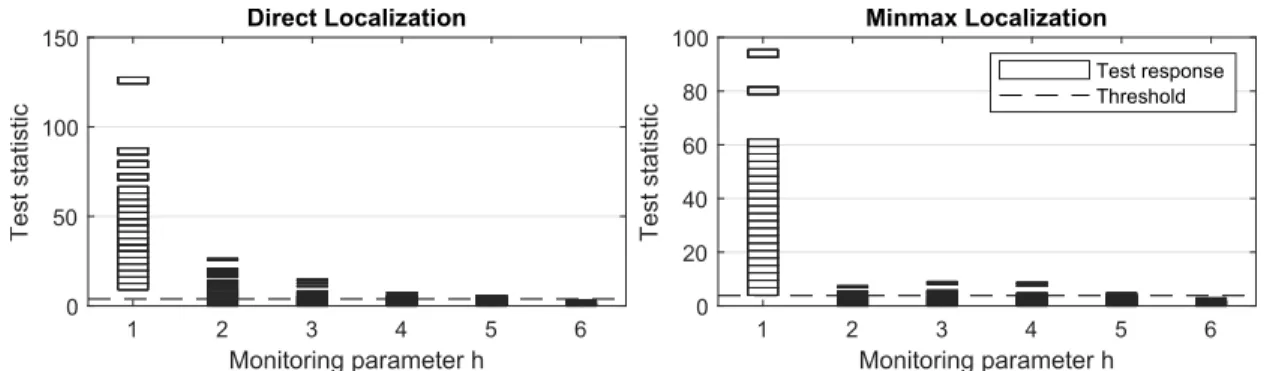
4.6 Damage localization of a 2% stiffness decrease in Spring 1 . . . 58
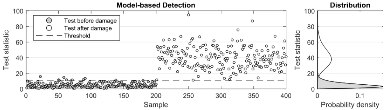
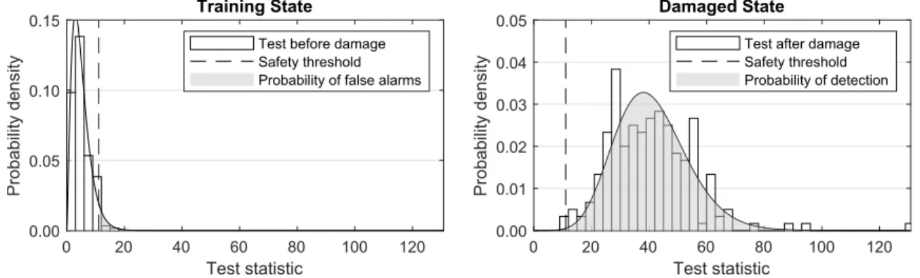
4.7 Probability of false alarms, safety threshold value, and probability of detection . . . 62
4.8 Flowchart for damage diagnosis . . . 63
5.1 Statistical distribution of the test statistic . . . 67
5.2 Minimum non-centrality as a code-based reliability index . . . 70
5.3 HSS beam with nine material properties and one sensor . . . 74
5.4 Numerical mode shapes and power spectral density of the generated signal . . . 74
5.5 Jacobian computation through the chain rule (reference state) . . . 76
5.6 Fisher information computation (reference state) . . . 76
5.7 Training state . . . 77
5.8 Validation state . . . 77
5.9 Validation state for the structural parametrization . . . 78
5.10 Training state . . . 78
5.11 Training state . . . 78
5.12 Validation state for the modal parametrization . . . 79
5.13 Validation state for the non-parametric test . . . 80
6.1 Statistical distribution of the test statistic for ν = 1 . . . 83
6.2 Comparing the minimum non-centrality for damage detection and localization . . . 86
6.3 Visualizing the hierarchical clustering . . . 90
6.5 Numerical HSS beam with nine materials and four sensors . . . 94
6.6 Numerical mode shapes and power spectral density of the generated signal . . . 94
6.7 Fisher information for the direct test (left) and the minmax test (right) . . . 95
6.8 Validation of the prediction for the direct localization test . . . 96
6.9 Validation of the prediction for the minmax localization test . . . 97
6.10 Original model (top) and substructured model (bottom) . . . 99
6.11 Objective functions for automated substructuring . . . 99
6.12 Validation of the automated substructuring approach . . . 100
7.1 Elements of reproduction of the genetic algorithm (GA) with integer sensor encod-ing and r = 3 sensors . . . 108
7.2 Flowchart for the genetic algorithm with a single objective . . . 110
7.3 Evolution of sensor layouts in the multi-objective GA . . . 111
7.4 Numerical HSS beam including the possible sensor locations P1 - P8 . . . 112
7.5 Numerical mode shapes . . . 112
7.6 Minimum measurement duration Th for (a) one sensor at position P2, and (b) two sensors at P1 and P8 . . . 113
7.7 Measurement durations T (c, r = 1) and standard deviations . . . 114
7.8 Optimal measurement time Topt(c) for a varying number of sensors . . . 114
7.9 Measurement durations T (c, r = 2) . . . 114
7.10 Test distribution for a 5% stiffness decrease in stiffness parameter E1 . . . 115
7.11 HSS beam including the possible sensor locations P1 - P24 . . . 116
7.12 Convergence chart for the genetic algorithm, showing the rank of elite members with respect to their ranking after an exhaustive search (ES) . . . 116
7.13 Schematic bridge with six possible sensor locations P1 - P6 . . . 117
7.14 Modes of vibration . . . 117
7.15 Feasible optimization space with 11 Pareto optimal solutions . . . 119
7.16 Empirically validating the mean test response to the minimum detectable damages 120 7.17 Test response to damage in a deck element (Parameter 6) and a hanger (Parameter 9) for balanced and tuned sensor layouts . . . 121
8.1 2-D Bernoulli beam in local coordinates (undeformed) . . . 126
8.2 Metal string with sensors S1 - S3 and support displacements u . . . 130
8.3 Numerical mode shapes and power spectral density of the generated signal . . . 130
8.4 Validation of the prediction for the minmax localization test . . . 131
8.5 Validating the Jacobian approximation . . . 131
8.6 Validation of the prediction for the minmax localization test . . . 132
8.7 Validating the Jacobian approximation . . . 132
8.8 Validation of the prediction for the minmax localization test . . . 132
8.10 Modes of vibration . . . 134
8.11 Localization of abutment settlement (left) and tower tilt (right) . . . 135
8.12 Validating the Jacobian approximation . . . 135
8.13 Localization of a loss in pretension in cables T1, T2, and T3 . . . 136
9.1 Laboratory HSS steel beam on pin supports . . . 139
9.2 Numerical HSS beam with eight sensor locations P1 - P8 . . . 141
9.3 Experimental power spectral density from eight sensors . . . 141
9.4 Numerical modal analysis with four sensors at P1, P2, P7, and P8 . . . 141
9.5 Block Hankel singular values . . . 142
9.6 Covariance singular values . . . 142
9.7 Fisher information matrix and its singular values . . . 142
9.8 Training procedure to determine the minimum measurement duration . . . 143
9.9 Damage scenarios with extra masses . . . 145
9.10 Validating the prediction for the damage detection tests . . . 145
9.11 Optimal substructure arrangement for K = 6 clusters . . . 149
9.12 Automated parameter clustering . . . 149
9.13 Minmax Fisher information with six clusters K = 6 and its singular values . . . 150
9.14 Damage localization . . . 150
9.15 Probability of detection for sensor configurations with rank 70, 36 and 1 . . . 152
9.16 Ranking all 70 configurations with r = 4 sensors . . . 152
9.17 Performance curve . . . 152
9.18 Relation between the mean test response and the measurement duration . . . 153
9.19 St. Nazaire Bridge (Janberg, 2020) . . . 155
9.20 Experimental setup for the St. Nazaire Bridge . . . 155
9.21 Finite element model of the St. Nazaire Bridge in MATLAB® . . . 156
9.22 First six modes of vibration in the vertical direction (FE Model) . . . 157
9.23 Repeated mode at about 80.5 Hz . . . 158
9.24 Automated clustering of cable cross-section parameters . . . 160
9.25 Non-centrality of the minmax localization test for damage scenario P19 . . . 160
9.26 Singular values of the Block Hankel matrix and the Fisher information . . . 161
9.27 Substructure arrangement for 20 parameter clusters . . . 162
9.28 Comparing the predicted and the measured non-centrality for ∆3 = 50% . . . 162
9.29 Validation state for all 36 damage scenarios . . . 163
10.1 Numerical HSS beam with nine materials and two sensors . . . 166
10.2 Numerical modal analysis . . . 166
10.3 Effect of changing time lags . . . 169
10.4 Minimum detectable damage and non-centrality ratio for increasing noise contam-ination. The noise is in percent of the output variance . . . 170
10.5 Subspace angles between the FEA-based observability and the data-driven column
space of the block Hankel matrix . . . 171
10.6 Fisher information for a simply supported beam with asymmetrical excitation . . . 172
10.7 Relation between the detectable damage and the number of modes . . . 173
10.8 Convergence of the predictions for a varying number of data segments . . . 175
10.9 Increasing the sampling frequency for a fixed measurement duration T (left side) and a fixed sample size (right side). Refer to Table 10.3 for input parameters . . . 176
10.10 Zero mean and unit variance checks in the training state . . . 179
10.11 Gaussianity check, goodness-of-fit test on the parametric residual . . . 179
10.12 Convergence of the minimum detectable damage . . . 180
10.13 Convergence of the Fisher information matrix norm and the covariance matrix norm181 10.14 Convergence of the Jacobian matrix norm . . . 181
10.15 Gaussianity convergence studies in the reference state . . . 183
10.16 Gaussianity convergence studies in the testing state . . . 184
10.17 Convergence of the non-centrality ratio in the testing phase . . . 184
10.18 Jacobian prediction error (JPE) for the change prediction in natural frequencies (shown for Parameter θ5) . . . 186
10.19 Jacobian prediction error (JPE) for the change prediction in mode shape coordi-nates (shown for Parameter θ5) . . . 186
10.20 Jacobian prediction error (JPE) for the change prediction in natural frequencies (shown for Parameter θ5) . . . 187
MATLAB
®MATLAB®is a registered trademark of The MathWorks, Incorporated, 3 Apple Hill Drive, Natick,
MA, 01760-2098, United States. Additional toolboxes include the Signal Processing Toolbox and the Global Optimization Toolbox.
https://www.mathworks.com/
ANSYS
®ANSYS® is a registered trademark of ANSYS, Incorporated, Southpointe 2600 Ansys Drive,
Canonsburg, PA 15317, United States. The Mechanical APDL interface is used in combination
with the aaS MATLAB® toolbox.
AL asymptotic local B.C. British Columbia
BCSIMS British Columbia Smart Infrastructure Monitoring System CDF cumulative density function
CLT central limit theorem DOF degrees of freedom
EOV environmental and operational variable ES exhaustive search
FE finite element
FEA finite element analysis GA genetic algorithm
GLR generalized likelihood ratio HSS hollow structural steel JPE Jacobian prediction error LTI linear and time-invariant NCR non-centrality ratio
NSGA-II 2nd generation of the non-dominated sorting genetic algorithm OMA operational modal analysis
PFA probability of false alarms POD probability of detection PSD power spectral density SHM structural health monitoring SNR signal-to-noise ratio
SSI stochastic subspace-based system identification SVD singular value decomposition
a, A Scalar
a Vector
aa Vector entry
A Matrix
Ai Matrix column i
A¯i Matrix with removed column i
Aij Submatrix
Aij Matrix entry in row i and column j
vec(A) Vectorization operator to stack columns in A
AT Transposed of A
A∗ Transposed conjugated complex matrix of A
A−1 Inverse of A
A† Pseudo inverse of A
Im Identity matrix of size m × m
A ⊗ B Kronecker product
R Set of real numbers
i Imaginary unit i2 = −1
Re(a) Real part of complex a
Im(a) Imaginary part of complex a
ˆ
X Estimate of variable X
¯
x, ¯X Complementary event or value of x or X
E(X) Expected value of a variable X
Eθ(X) Expected value of variable X under system parameter vector θ
N (µ, σ) Gaussian distribution with mean value µ and standard deviation σ
N (µ, Σ) Multi-dimensional Gaussian distribution with mean value vector µ and
covari-ance matrix Σ
χ2(ν) Central chi-squared distribution with ν degrees of freedom
χ2(ν, λ) Non-central chi-squared distribution with ν degrees of freedom and
A State transition matrix
B Input matrix
c, C1 Damping coefficient and damping matrix
C Output matrix
C Controllability
D Feed-through matrix
h Parameter number h = 1, 2 . . . , H
H Block Hankel matrix
J Sensitivity matrix (Jacobian)
k, K Stiffness and stiffness matrix
k Cluster number k = 1, 2 . . . , K
m, M Mass and mass matrix
N, N0 Number of samples during training and testing
Nm Number of modes of vibration
O Observability
p Time lag for block columns in block Hankel matrix
q Time lag for block rows in block Hankel matrix
r, r0 Number of uni-axial sensors, number of projection sensors
S Singular values
U0 Left null space
U Left singular vectors
V Right singular vectors
α False-positive rate (type I error)
β False-negative rate (type II error)
δ Statistical change vector
ε Residual vector
ζ Critical damping ratio
ζ Gaussian residual vector
η Parameter vector with modal parameters
θ Parameter vector with structural design parameters
First of all, I would like to thank my research supervisor Carlos Ventura for his support and confi-dence in my work. He inspired the research proposal and guided me through the challenges of the research program. I am appreciative that he put emphasis on both my academic and professional development by involving me in client projects, and trusted me with valuable measurement equip-ment. I will be forever grateful for the conferences he sent me to, and the professional network
he helped me build. Particular thanks go to my co-supervisor Michael D¨ohler for his inspiration,
mentoring, and patience. His originality, academic excellence, and thoroughness were a humbling experience and driving force throughout my thesis. His supervision and mentoring has set an un-precedented standard. The work environment and team spirit at Inria have shaped my perception of the academic world and left a lasting imprint on my personality.
Furthermore, I would like to express my gratitude for the support I received from my supervi-sory committee members and the subtle impulses they gave me whenever I needed them. I truly enjoyed the discussions with Ruben Boroschek and his strong and well-founded opinion. Reza Vaziri’s knowledge on finite element analysis were extremely helpful. It was a great pleasure to assist Terje Haukaas with teaching, and his knowledge on statistical analysis is much appreciated. Special thanks go to Yavuz Kaya for his supervision in the first year and the insights into the plans of the Ministry of Transportation and Infrastructure. On this occasion, I would like to acknowledge my colleagues at UBC and Inria. Special thanks go to the Manager of the Earthquake Engineer-ing Research Facility, Mehrtash Motamedi, and Project Assistant Terry Moser, who were always available, responsive, and supportive. I would also like to thank my Team Leader at Inria, Laurent Mevel, for his enthusiasm for my work and his mentorship. His many ideas, his point of view, and profound knowledge were a great source of inspiration. Special thanks go to my colleagues Szymon
Gre´s and Eva Viefhues, whose work and expertise I greatly benefited from. Equally, I would like
to thank Fr´ed´eric Gillot who selfishly helped me through discussions on global optimization.
Finally, I would like to thank my family. My parents Ludwig and Susanne Mendler encouraged me to commence the PhD program and supported me throughout it, despite the sacrifices this meant for them. Due to the large distance, I was unable to say my goodbyes to my grandparents Heinz Kobiela and Lotte Mendler, who deserve to be acknowledged here. Special thanks also go to my grandmother Irmgard Kobiela for her continuous financial support. At the end of this list— though really at the beginning of it all—stands my loving partner and best reader, Jennifer Mah, without whom this thesis would not exist.
Background
“A society grows great when old men plant trees whose shade they know they shall never sit in.”
— Greek Proverb
1.1
Introduction
The province of British Columbia (B.C.) is located in one of the most seismically active zones in Canada and the world, and is dependent upon lifeline infrastructure that bridges the coastal rivers and the Pacific inlets. Many of the existing links are designed according to outdated design standards, e.g., the George Massey Tunnel, or are nearing the end of their design basis service life, e.g., the Lion’s Gate Bridge and the Second Narrow’s Bridge. Since these structures cannot be economically replaced, or because of their iconic value, techniques for bridge monitoring are developed so their operation can be extended beyond their original lifespans.
In the context of civil engineering structures, the process of implementing a damage diagno-sis strategy is referred to as structural health monitoring (SHM). Due to the existing monitor-ing system, this work focuses on vibration-based damage diagnosis. This process involves the observation of the structural vibrations through permanently installed sensors, the extraction of damage-sensitive features, and their subsequent statistical evaluation (Farrar and Worden, 2012). The statistical evaluation includes a data normalization step that removes the effect that changing environmental and operational variables (EOVs) have on the vibration behaviour of the structure (e.g., wind, traffic loads, temperature fluctuations, icing). Some features are robust to changes
to EOVs (Balm`es et al., 2008a, 2009; Viefhues et al., 2020), which is why they are not explicitly
considered in this thesis. The damage diagnosis involves four consecutive steps with increasing complexity, i.e., damage detection, localization, quantification, and the prediction of the remain-ing lifetime (Rytter, 1993). The real-time information on the health state increases the structural safety between periodically scheduled bridge inspections, and allows for a coordinated emergency response after extreme events, such as storms, tsunamis, or earthquakes. For the urban communi-ties in the Southwest of B.C., the advancement of a bridge monitoring network (and with it, the theoretical developments in SHM) are particularly relevant because there is a one out of ten chance that a megathrust earthquake will strike within the next 50 years (Onur and Seemann, 2004). All emergency response and evacuation services depend on a few lifeline bridges that will turn into the most critical and vulnerable infrastructural links.
SHM poses multiple challenges specific to civil engineering structures. Firstly, no site and bridge are identical, so a structure-specific training of the damage diagnosis algorithm is required, and findings from one bridge cannot straightforwardly be applied to another. Therefore, it is challenging to assess whether certain damages can or cannot be detected and localized querying the value of implementing a SHM system. Secondly, due to the sheer size of bridges, a dense sensor layout cannot be realized and local monitoring approaches cannot be applied, so global monitoring approaches are to be applied in combination with sparse sensor layouts that are strategically laid out for successful damage detection. For instance, the Port Mann Bridge exhibits a length and width of 2,020 m and 65 m, respectively, and 288 stay cables, but the acquisition and maintenance costs for monitoring each cable using local damage diagnosis methods are unreasonable. Thirdly, a lack of real vibration data from damaged structures is impeding the research progress, as bridges are vital links in primary infrastructure and damaging them for research purposes, as it was done in the case of the Z24 Bridge in Switzerland and the S-101 Bridge in Austria, can only be justified after exceeding their life expectancy. Equally, continuous operation is imperative, and bridge closures for dynamic or static testing are unacceptable. Consequently, the damage diagnosis is to be performed during normal operating conditions and under unknown force excitation. With this in mind, this thesis pursues the following objectives:
Objective I: Build a universal framework, which is applicable to a wide range of structures, damage-sensitive features, and anticipated damage scenarios, to calculate the minimum de-tectable and localizable damage based on global vibration monitoring
Objective II: Devise criteria that describe the detectability and localizability of damage and incorporate them into a sensor placement optimization scheme for large mechanical systems Objective III: Implement self-validation strategies to test the applicability of the algorithm for
real structures, to verify input parameter settings, and to non-invasively test its performance in the absence of damage
All considerations are made for a damage diagnosis method, called the asymptotic local (AL) approach using the subspace-based residual as a damage-sensitive feature. This method allows for an online evaluation with diagnostic capabilities including detection, localization, and quantifica-tion. However, all developed tools are universal in that they can be applied to any damage-sensitive feature with Gaussian properties. The tools are of great value to predict the minimum detectable and localizable damage, to optimize the sensor placement, and to assess the value of SHM for bridge monitoring in general. Ultimately, all methods are readily applicable to other civil engineer-ing structures, such as buildengineer-ings, offshore structures, defence systems, minengineer-ing structures, or power plants, as well as mechanical structures such as ships, aircraft, and spacecraft.
(a) Significant historic earthquakes (b) Relative seismic hazard map
Figure 1.1: Seismic hazard in British Columbia (B.C.) (Earthquakes Canada, 2020)
1.2
Motivation
The Southwest of B.C., including Vancouver and the densely populated Fraser River delta, is one of the most seismically active regions in Canada (Clague et al., 1998). About 150 km off the coast of Vancouver, a locking mechanism at the tectonic plate interfaces causes strain to be built up continuously. Geologic evidence has shown that the strain is released abruptly every 300 - 700 years through subduction interface earthquakes with magnitudes of up to 9.0, with the last one occurring in 1700 (Goldfinger et al., 2012). The relative movement between the two plates since then amounts up to 12 m. Smaller, but still damaging earthquakes within the overlapping crust, or deep down in the subducting slab are omnipresent reminders of the seismic threat. The four most recent and significant ones are the 2001 Nisqually earthquake (M = 6.8), the 1965 Puget Sound earthquake (M = 6.7), the 1949 Olympia earthquake (M = 6.7), and the 1946 Vancouver Island earthquake (M = 7.3), see Fig. 1.1. At the same time, the seaport city is located on a peninsula that is wedged between the Pacific Inlet, coastal mountains and the Fraser River delta, causing the two sea bridges and four river bridges across the 400 m wide main arm of the Fraser River to be among the largest and widest in North America (Svensson, 2013), see Figure 1.2. For example, when the Alex Fraser Bridge was opened to traffic in 1986, it was the longest cable-stayed bridge in the world. The Golden Ears Bridge was opened to traffic in 2009, and is still the longest extra-dosed bridge in North America. Last but not least, with a width of up to 12 traffic lanes (65 m), the Port Mann highway bridge was the widest bridge ever built at the time of its inauguration in 2012, and is still the second longest cable-stayed bridge in North America.
1.2.1 Lifeline Bridges
The bridge monitoring in B.C. follows the lifeline monitoring philosophy. The highway bridge in-ventory of British Columbia was evaluated in 2017 (Siddiquee et al., 2017) and the report concludes
WEST
VANCOUVER VANCOUVERNORTH
VANCOUVER RICHMOND LANGLEY ABBOTSFORD SURREY DELTA BURNABY COQUITLAM MISSION WHITE ROCK NEW WEST-MINSTER Pitt River Queensborough QB Connector Alex Fraser No 2 Road Dinsmore Bridge 2nd Narrows Granville Burrard Cambie Arthur Laing Moray MAPLE RIDGE
Disaster response route (federal) Disaster response route (municipal) Symbol for bridge
Symbol for tunnel Lifeline structure Cable-supported bridge Legend (last update: April 2018)
Name
Lion's Gate
Golden Ears
George Massey tunnel Knight Street Oak Street
Port Mann Patullo
Figure 1.2: Major-route and lifeline bridges of Metro Vancouver, Canada
that 80% of all highway bridges are between 20 m and 100 m long and exhibit simple structural systems, such as simply-supported or continuous multi-span girders. The numbers suggest these bridges are the most relevant infrastructures; however, more than 68% of the population lives in the Southwest of B.C., and among those, two out of three live in Metro Vancouver (Foster et al., 2011), where merely 20.4% of all bridges are located, see Fig. 1.2. The seismic hazard is the greatest in the coastal areas (Earthquakes Canada, 2020), but only 26.5% of all bridges are located here, Figure 1.1b. Since the area with the highest population density overlaps with the most seismically active zone, the bridge design code categorizes the safety requirements for bridges with respect to their importance. On the bases of social, economic and security requirements, the seismic design guidelines distinguish between three importance categories: (a) lifeline bridges, (b) major-route bridges, and (c) other bridges. Major-route bridges are part of the municipal and federal disaster response network and are required to facilitate emergency response and defence purposes. In the event of an earthquake or tsunami, they are designated for use by emergency personnel only, and they are not used for evacuation purposes. Lifeline bridges, on the other hand, serve the general public. They are vital to the integrity of the local transportation network and the ongoing econ-omy. Moreover, particularly large (and expensive) or iconic bridges can be declared lifeline bridges. The importance category determines the design approach and the analysis requirements. More importantly for monitoring applications, it also determines the performance levels, which describe the accepted level of damage as well as the serviceability requirements after an earthquake has
Prob. Lifeline bridges Major-route bridges Other bridges in 50 a Lvl. Serviceability Damage Lvl. Serviceability Damage Lvl. Serviceability Damage 10% (1) Immediate None (2) Immediate Minimal (3) Limited∗ Repairable∗ 5% (2) Immediate Minimal (3) Limited∗ Repairable∗ (4) Disrupted∗ Extensive∗ 2% (3) Limited Repairable (4) Disrupted Extensive (5) Life safety Replacement
∗Optimal performance levels unless required by the Regulatory Authority or the Owner Table 1.1: Performance levels for bridges as per (S6-19, 2019)
occurred. In the case of a megathrust earthquake (with a probability of exceedance of 2% in 50 years), lifeline bridges are required to remain operational with minor service limitations and re-pairable damage. In contrast, non-essential bridges are expected to be closed to traffic and replaced in the aftermath of a megathrust earthquake, refer to Table 1.1. The maintenance effort of bridges correlates with bridge area, and an estimation yielded that 24.3% of all lifeline bridges in Metro Vancouver are already cable supported (neglecting the approach viaducts, this number increases to 53.2%) and additional cable-stayed bridges are in planning. Three out of the six disaster response bridges (major-route bridges) are cable-stayed and so are all bridges across the main arm of the Fraser River—the main evacuation route.
To summarize, the efficiency of disaster response services and the safety of evacuation procedures for a majority of the population depend on the structural health state of cable-stayed bridges, and the ability to assess them rapidly. It would be invaluable for the city of Vancouver and B.C. to have an algorithm in place that can reliably detect and localize damage, and rank the bridges according to the severity of damage sustained during an earthquake.
1.2.2 Monitoring System
In 2009, the B.C. Ministry of Transportation & Infrastructure embarked on a program called the British Columbia Smart Infrastructure Monitoring System (BCSIMS). The resulting online platform makes available the data of two monitoring networks, including a strong motion network with 162 accelerometers and a structural health monitoring network with 15 bridges and one tunnel (Kaya et al., 2017). The instrumentation on the bridges is designed to capture the global vibration behaviour, in order to record strong ground motions and their effect on both the structures and the soil. All sensors record the structural response of the bridges (< 200 Hz) to ambient excitation.
The primary objective of the SHM network is to provide a post-earthquake damage assessment module which assesses the structural health state in real-time, and thus, enable prioritized bridge inspections and rapid deployment or repair measures (Kaya et al., 2017). The second objective is the long-term monitoring for cost-efficient operation over the entire life span of bridges and schools, see Figure 1.3. The monitoring data is supposed to supplement the regular bridge inspections, and aid with the estimation of the remaining lifetime. The existing monitoring system is an excellent database for research in the field of vibration-based damage diagnosis but no damaging events have been recorded to date.
Existing Monitoring Network
Strong motion monitoring Pacific Geoscience Centre, Geologic Survey of Canada
Structural health monitoring University of British Columbia and MoT
Public Schools Lifeline Bridges Lifeline and Major-route Bridges Module 2: Dynamics-based Damage Assessment Real-time monitoring for postearthquake damage assessment Module 1: Probabilistic Damage Prediction Long-term monitoring for cost-effective operation over the
entire life span
Roadmap for Bridge Monitoring
BCSIMS Ministry of Transportation & Infrastructure Earthquake Early-warning Other Tools
Figure 1.3: Architecture of the B.C. Smart Infrastructure Monitoring System (BCSIMS)
1.2.3 Anticipated Damage
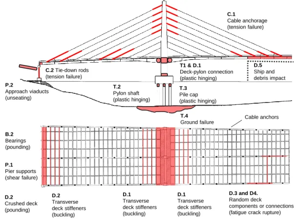
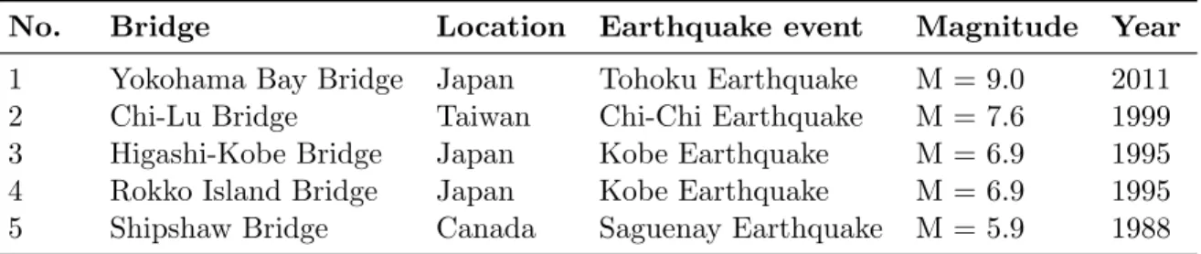
The development of an efficient SHM system requires knowledge of probable damage scenarios dur-ing earthquakes. This section summarizes the finddur-ings from a literature review on post-earthquake damage on the five cable-stayed bridges in Japan, Taiwan, and Canada, listed in Table 1.3. All documented damage scenarios are illustrated in Fig. 1.4.
D.3 and D4.
Random deck
components or connections (fatigue crack rupture)
T1 & D.1 Deck-pylon connection (plastic hinging) C.2 Tie-down rods (tension failure) P.2 Approach viaducts (unseating) T.3 Pile cap (plastic hinging) T.2 Pylon shaft (plastic hinging) C.1 Cable anchorage (tension failure) T.4 Ground failure D.2 Transverse deck stiffeners (buckling) P.1 Pier supports (shear failure) D.1 Transverse deck stiffeners (buckling) D.5 Ship and debris impact D.1 Transverse deck stiffeners (buckling) D.2 Crushed deck (pounding) B.2 Bearings (pounding) Cable anchors
Component ID Location Failure mechanisms
Damage symptoms Severity*
Deck D.1 Deck-pylon
connection
Flexural hinging shear failure
Stiffness reduction, concrete spalling, yielding and buckling of reinforcement
(5)
D.2 Deck-pier
connection
Shear failure, and pounding
Buckling and cracking of transverse beams and end beams, crushing of main girders and the concrete slab in the longitudinal direction
(4)
D.3 Main girder Fatigue crack
rupture
Stiffness reduction of main girders due to partial or complete rupture
(4)
D.4 Girder
connection
Fatigue crack rupture
Stiffness reduction of steel joints due to partial or complete rupture
(3)
D.5 Shipping lane Ship and debris
impact
Large deformation of main girders and transverse floor beams, buckled stiffeners, concrete spalling
(5)
Deck bearings B.1 At main pylon Pounding Crushed wind shoes, concrete spalling on
deck and pylons
(3)
B.2 At pier Pounding Crushed wind shoes (3)
Main tower T.1 Pylon-deck
connection
Flexural hinging and shear failure
Stiffness reduction, concrete spalling, yielding and buckling of reinforcement
(5)
T.2 Pylon shaft Flexural hinging
and shear failure
Reduced cross section due to concrete spalling
(5)
T.3 Pile caps Plastic hinging and
cracking due to rocking or fence posting
Horizontal cracking of pile caps (4)
T.4 Entire tower Ground failure due
to settlements, liquefaction, landslides, etc.
Vertical pylon settlement up to 6 m, residual horizontal displacements, or rotations
(5)
Stay cables C.1 Cable anchors Tension failure at
the main span
Cross section reduction (due to strand failure), or slacking of entire cables near anchors
(3)
C.2 Tie-down
rods at piers
Tension failure Loss of prestress in anchor cables, and uplift
of the deck from the pier support
(5)
End-span piers P.1 Pier supports Shear failure due to
horizontal and vertical pounding
Crushing of bearings, cracking of transverse pier beams, buckling or shear failure of supporting columns
(5)
P.2 Approach
viaducts
Displacements and rotations of the pier foundations
Partial or total collapse of simply-supported approach spans (unseating)
(5)
∗maximum expected damage potential expressed with respect to the performance classes defined in the Canadian highway bridge design code Table 1.2: Anticipated earthquake damage on cable-stayed bridges, refer to Fig. 1.4
No. Bridge Location Earthquake event Magnitude Year
1 Yokohama Bay Bridge Japan Tohoku Earthquake M = 9.0 2011
2 Chi-Lu Bridge Taiwan Chi-Chi Earthquake M = 7.6 1999
3 Higashi-Kobe Bridge Japan Kobe Earthquake M = 6.9 1995
4 Rokko Island Bridge Japan Kobe Earthquake M = 6.9 1995
5 Shipshaw Bridge Canada Saguenay Earthquake M = 5.9 1988
Table 1.2 gives details on each damage scenario shown in Fig. 1.4. It includes the failure mechanism and observed damage symptoms, and assesses the damage consequences with respect to the performance levels in the bridge design code S6-19 (2019) from Table 1.1. For example, the observed damage scenarios on stay cables are categorized into anchor failure (C.1) or failure of tie-down rods (C.2). The failure mechanism is tension failure, and observable damage symptoms include slack cables and strand failure or uplift of the deck from the pier supports, respectively. Cable-stayed bridges are redundant structural systems, so individual cable anchorage failure may lead to limited serviceability, but allow the damage to remain repairable—in other words, cable anchorage failure satisfies performance level 3 of the bridge design code (see Table 1.1). On the other hand, failure of tie-down rods, as it occurred on the Shipshaw Bridge in Canada, can lead to bridge collapse, which affects the life safety and requires a bridge replacement (Level 5 in Table 1.1). Consequently, the monitoring system should be tuned to become more sensitive to damages in local key components with Level 5 consequences on the safety and serviceability of the structure, and the sensor placement should be optimized accordingly. Another observation is that damage accumulates at stiffness discontinuities, such as cable anchors and tie-down rods, joints between different bridge components (tower, deck, foundations), and bearings. Such damage hotspots should be monitored more closely.
1.3
Methodology
1.3.1 Damage Diagnosis
Vibration-based SHM is divided into three stages: (1) the observation of the dynamic system through sensors, (2) the feature extraction, and (3) the statistical evaluation of the features. The statistical evaluation is referred to as the damage diagnosis, where damage is understood as a de-terioration of structural design parameters, such as material constants (Farrar and Worden, 2012), cross-sectional values, prestressing forces (Chen and Duan, 2014), support conditions, and mass-distribution parameters (Santos et al., 2013). The primary task of damage diagnosis is to detect the presence of damage, and more advanced tasks include the narrowing down of the exact damage location (localization) and the quantification of its extent. The selected damage diagnosis method is based on the AL approach (Benveniste et al., 1987), with diagnostic capabilities including
detec-tion (Basseville et al., 2000), localizadetec-tion (Basseville et al., 2004), and quantificadetec-tion (D¨ohler and
Mevel, 2015). It is based on a similar framework as stochastic subspace-based system identification (SSI), which has developed into a powerful algorithm for the system identification under unknown excitation since the publication of the book by van Overschee and de Moor (1995). The diagnosis method is applied in combination with the subspace-based residual, which circumvents the lengthy estimation of dynamic properties (e.g., natural frequencies), and thus, allows for an online evalu-ation in real-time. The measurement quantities can be accelerevalu-ations, velocities, or displacements. More reasons for the choice of this method are given in Section 2.1.2.
1.3.2 Contributions
This thesis aims to build a framework to analyze the minimum diagnosable damage, i.e., the minimum detectable and localizable damage. All considerations are made based on vibration data from the undamaged structure in combination with a finite element model. This avoids empirical and structure-specific experiments, and makes the framework universally applicable to a wide range of civil and mechanical engineering structures, damage-sensitive features, and anticipated damage scenarios from Fig. 1.4. Most considerations target the performance assessment before a SHM
system is installed. However, additional self-validation strategies are implemented to test the
applicability of the algorithm to real structures, to verify the input parameters, and to test its performance based on non-invasive tests.
All contributions rely on the particular strength of the asymptotic local (AL) approach; it allows for a comprehensive treatment of statistical uncertainties in the damage-sensitive feature, and includes structural information from finite element (FE) models. Hence, the AL approach is not a black box algorithm but considers the physical properties of the considered structure. All contributions are listed in the following:
(1) Minimum Detectable Damage. The minimum detectable damage is defined as the mini-mum change in structural design parameters that can be reliably detected based on changes
in the damage-sensitive feature. No site and structure are identical, so a structure-specific
training of the damage diagnosis algorithm is required and findings from one structure cannot straightforwardly be transferred to another. Consequently, it is challenging to assess whether or not certain damages can or cannot be detected and localized before the SHM system is installed, making it hard to convince decision-makers of the benefits. Furthermore, statistical uncertainties are typically quantified through empirical approaches or rules of thumb, but they are challenging to validate. With this background, a formula is developed in this thesis that allows for the prediction of the test response to damage based on vibration measure-ments from the undamaged structure. When combined with a reliability concept, including the probability of false alarms (PFA) and a minimum probability of detection (POD), the minimum detectable damage can be predicted. Among other factors, the predictive frame-work considers the signal-to-noise ratio of the vibration measurements, and the measurement duration during testing. The prediction of the minimum detectable damage requires a FE model, but is also valid for purely data-driven tests.
(2) Minimum Localizable Damage. Damage localization is more complicated than dam-age detection. The minimum localizable damdam-age is defined as the minimum change in a structural design parameter that can be detected and distinguished from changes in other parameters under an optimal damage localization resolution. A fundamental problem is the over-parametrization of FE models. That means that multiple structural design parameters in the model have a similar effect on the damage-sensitive feature, and, vice versa, it is challeng-ing to identify the design parameters that have changed. The problem can be addressed by
clustering the design parameters, which corresponds to a substructuring of the finite element model into damage localization units, in which damage can be isolated. However, this thesis shows that finding the optimal substructuring arrangement is a multi-objective optimization problem: with an increasing number of substructures, the damage localization resolution increases, but the damage detectability in each substructure decreases. Moreover, an inap-propriate substructure arrangement can lead to false localization alarms, which can obscure the actual damage location. The issue is addressed by expanding the predictive framework for the minimum detectable damage to damage localization. Additional considerations are made so the magnitude of false alarms can be predicted based on reference data. Ultimately, a multi-objective optimization scheme is introduced (based on Pareto optimization) to auto-matically find the optimal substructure arrangement as a compromise between localization resolution, damage detectability, and false alarm susceptibility.
(3) Sensor Placement Optimization. Damage detectability and localizability based on global structural vibrations critically depends on the sensor layout. The sensor layout determines the observability of structural modes of vibration, which carry valuable information on local design parameters. In particular, if a small number of sensors is used to monitor large structures, an optimized sensor layout ensures optimal coverage of all monitored design parameters. Many optimization criteria aim to precondition the signal and the signal-to-noise ratio. Some criteria increase the quality of the system identification with minimum uncertainty. Only a few criteria seem to optimize the damage detectability and the probability of detection. However, none of the existing criteria appear to consider the relative decrease in material strength, although this is the decisive quantity for structural design, structural health, and
thus, safety. Another issue is that most sensor placement strategies optimize the sensor
layout to capture the global vibration behaviour. Still, the structural safety and serviceability typically depend on the integrity of local key components, such as joints, and damage tends to accumulate at well-known hotspots, see Fig. 1.4. Therefore, a sensor placement strategy is developed in this thesis that takes as input the requested detectable damage in individual FE model components, and yields as output the corresponding optimal sensor layout. This strategy maximizes the damage detectability and localizability, and can be employed to find the optimal sensor layout as well as an appropriate number of sensors.
(4) Monitoring Boundary Conditions. Change in boundary conditions, i.e., a loss in pre-tension or support displacements, is a typical damage scenario during extreme events such as earthquakes, see Fig. 1.4. Moreover, excessive support settlements or loss of tension in prestressing tendons (due to slippage or stress corrosion) are common problems in bridge monitoring. Changes in boundary conditions have a global characteristic, as they lead to a global re-distribution of stiffness. Detecting global changes in the dynamic response measures based on global damage diagnosis methods is unproblematic, but distinguishing them from local structural changes is a challenge. In this light, an approach is put forward to calculate
the sensitivity of the damage-sensitive residual toward changes in boundary conditions. The resulting sensitivity vectors can be incorporated into the existing damage diagnosis frame-work of the AL approach, enabling both the localization of changes and the prediction of the minimum diagnosable changes.
(5) Model Validation. Bridges are vital links in primary infrastructure and damaging them
for research purposes is generally not an option. Due to each structure’s uniqueness, it
is challenging to verify whether the theoretical assumptions are fulfilled and whether all
input parameters for signal processing are set appropriately. To address the issues, this
thesis proposes the application of extra masses as a non-invasive validation technique, and demonstrates the effectiveness based on a laboratory experiment on a steel beam. Moreover, another strength of the predictive framework is showcased by introducing a series of tools and quick checks to verify the input parameter choice based on numerical simulations.
1.3.3 Thesis Organization
The thesis is organized into three parts. Part I. includes a state-of-the-art review of global damage diagnosis methods and existing sensor placement strategies (Chapter 2). An introduction to struc-tural dynamics from a control theory perspective is given (Chapter 3), as well as an introduction to damage diagnosis using the asymptotic local approach (Chapter 4). Part II. presents the the-oretical contributions of this research project and is divided into the minimum detectable damage (Chapter 5), the minimum localizable damage (Chapter 6) and optimal sensor placement (Chap-ter 7). In addition, an approach is outlined to incorporate changes in boundary conditions into the damage diagnosis framework of the asymptotic local approach (Chapter 8). Part III. summarizes practical investigations. First, two case studies are presented (Chapter 9), including a laboratory steel beam and a laboratory cable-stayed bridge. Secondly, self-validation studies are summarized (Chapter 10), and ultimately, the particular strength and limitations of all methods are highlighted in the conclusions (Chapter 11).
Literature Review
“If I had eight hours to chop down a tree, I’d spend the first six of them sharpening my axe.”
— Abraham Lincoln
This work develops a strategy to analyze the minimum detectable damage for vibration-based structural health monitoring (SHM) and to optimize the sensor layout. Both fields are extensively researched. The review is split into two parts: the first part (Section 2.1) revisits existing damage-sensitive features and damage diagnosis methods, and gives reasons for the choice of the asymptotic local (AL) approach. Moreover, existing strategies are touched upon to diagnose changes in bound-ary conditions, together with previous attempts to quantify the minimum diagnosable damage. The second part (Section 2.2) reviews existing performance criteria and smart optimization algorithms to overcome the problem of combinatorial explosion in large mechanical structures.
2.1
Global Vibration-based Damage Diagnosis
The premise of vibration-based damage diagnosis is that damage alters the stiffness, mass, or damping properties of the structure. Consequently, structural changes can be inferred based on the global system response. The process of damage diagnosis is divided into data acquisition, the extraction of damage-sensitive features, and their statistical evaluation (Farrar and Worden, 2012). Depending on the method, the removal of environmental and operational variables (EOVs) on the damage-sensitive feature is considered a separate step, or integrated into the damage diag-nosis method. Correspondingly, this section distinguishes between damage-sensitive features and diagnosis methods. The literature review focuses on global vibration-based SHM, as this work is motivated by the specific needs of the British Columbia Smart Infrastructure Monitoring System (BCSIMS). It is based on recent reviews by An et al. (2019) and Moughty and Casas (2017b), and preceding works by Fan and Qiao (2011), Carden and Fanning (2004), Chang et al. (2003), and Doebling et al. (1996), with a comprehensive overview in Farrar and Worden (2012).
2.1.1 Damage-sensitive Features
For an overall picture, Table 2.1 categorizes the presented damage-sensitive features, where the columns are sorted in ascending order with respect to the signal processing effort. Basic signal statistics form the first category (column 1). Farrar and Worden (2012) summarize that damage causes the peak amplitude to change, as well as the mean, the root mean, and the root mean square
Global Damage-sensitive Features Signal statistics Transient signals Waveform compar-isons Times series models Modal parame-ters Modal parameter based Peak amplitude Energy (Arias intensity) Response data Auto-regressive models Resonance frequencies Mode shape curvature Mean, root mean, root mean square Higher temporal moments Covariance function State space marices Mode shapes Strain energy Variance, standard deviation Vibration intensity Power spectral density Observ-ability matrix Damping ratios Modal flexibility Skewness, kurtosis Destructive potential factor Operating deflection shapes Kalman filter innovations Ritz-vectors Yuen functions Crest factor, K-factor Decay measures Modal force vector
Table 2.1: Damage-sensitive features (Farrar and Worden, 2012)
values. Mattson and Pandit (2006) argues that higher statistical moments (such as the standard deviation, skewness, and kurtosis) are more sensitive to damage than the mean or the variance. Pachaud et al. (1997) employs the crest factor and K-factor as measures of the signal’s deviations from the sinusoidal response.
Transient signals form another group, including measures for energy and intensity (column 2). Smallwood (1994) discusses energy measures and higher temporal moments. Moughty and Casas (2017a) perform damage detection on the S-101 bridge using the Arias intensity, vibration intensity, cumulative absolute velocity, destructive potential factor, and others. Farrar and Worden (2012) summarize multiple measures based on the decay of vibration signals, including the 10% duration time and the Hilbert transform.
Waveform comparisons can be made in either the time-domain or frequency-domain (column 3). This includes power spectral density (PSD) as well as covariance functions, and the direct signal response to random excitation. Yin and Tang (2011) evaluate the system response to passing vehicles. Pascual et al. (1999) suggest operating deflection shapes for damage detection to avoid modal identification. Basseville et al. (2000) form a damage-sensitive residual based on the
covari-ance matrix, and D¨ohler et al. (2014b) propose a similar feature that is more robust to changes
covariance function difference.
Time series models can be used as damage-sensitive features (column 4 in Table 2.1) after fitting them to the vibration record using regression techniques. For example, Fanning and Carden (2001) use the mean and the variance of the auto-regressive (AR) term as a damage-sensitive criterion. Spiridonakos and Chatzi (2015) employ non-linear AR models and minimized the simulation error. Equivalently, stochastic state space models can be employed. For example, Mehra and Peschon (1971) propose the Kalman filter innovations as damage-sensitive criteria. Swindlehust et al. (1995) use the observability as a damage-sensitive matrix for model updating. Time series-based models are suited to detect damage scenarios with non-linear characteristics and to distinguish them from linear changes due to EOVs (Figueiredo et al., 2011).
Modal parameters were among the first damage-sensitive features, and remain state-of-the-art (column 5). Adams et al. (1978) and Cawley and Adams (1979) initialize damage detection based on frequency changes. Since changes in mode shapes are less intuitive to track, Allemang and Brown (1982) propose a correlation measure, called the modal assurance criterion (MAC) for their evaluation, and Lieven and Ewins (1988) put forward a coordinate-by-coordinate MAC, called the coordinate modal assurance criterion (COMAC). Yuen (1985) combines frequencies and mode shapes into a criterion known as the Yueng function. Zouari et al. (2009) consider damping estimates, and Cao and Zimmerman (1999) use load-dependent Ritz vectors (or Lanczos vectors). Ojalvo and Pilon (1988) generate a modal force vector by confronting data-driven frequencies and mode shapes with model-based mass and stiffness matrices. While frequencies are more sensitive to damage than mode shapes (Cury and Cremona, 2012), mode shapes are less sensitive to EOVs (Deraemaeker et al., 2008) and include spatial information (An et al., 2019). Damping is non-linearly influenced by the vibration amplitude (Eyre and Tilly, 1997), and an accurate estimation
often fails under unknown force inputs (Brincker and Ventura, 2015). In general, quantifying
uncertainties in the modal parameters is equally as important as estimating them (Mellinger et al., 2016).
Features derived from modal parameters constitute the last category of features (column 6). Pandey et al. (1991) propose the mode shape curvature, which amplifies discontinuities in mode shapes by deriving them. Pandey and Biswas (1994) follow-up on this by introducing the modal flexibility method. Stubbs et al. (1992) employ the modal strain energy, which exhibits a higher sensitivity to local damages than modal parameters (Yam et al., 1996).
2.1.2 Damage Diagnosis Methods
The presented damage diagnosis methods are categorized into statistical pattern recognition (in-cluding supervised and unsupervised learning), finite element (FE) model updating, parametric change detection, and stochastic load vectors. The diagnosis depth is generally divided into four hierarchical steps with increasing complexity (Rytter, 1993):