HAL Id: hal-00298089
https://hal.archives-ouvertes.fr/hal-00298089
Submitted on 13 Sep 2007
HAL is a multi-disciplinary open access
archive for the deposit and dissemination of
sci-entific research documents, whether they are
pub-lished or not. The documents may come from
teaching and research institutions in France or
abroad, or from public or private research centers.
L’archive ouverte pluridisciplinaire HAL, est
destinée au dépôt et à la diffusion de documents
scientifiques de niveau recherche, publiés ou non,
émanant des établissements d’enseignement et de
recherche français ou étrangers, des laboratoires
publics ou privés.
amplitudes in Northern Eurasia inferred from
geothermal data
D. Y. Demezhko, D. G. Ryvkin, V. I. Outkin, A. D. Duchkov, V. T. Balobaev
To cite this version:
D. Y. Demezhko, D. G. Ryvkin, V. I. Outkin, A. D. Duchkov, V. T. Balobaev. Spatial distribution
of Pleistocene/Holocene warming amplitudes in Northern Eurasia inferred from geothermal data.
Climate of the Past, European Geosciences Union (EGU), 2007, 3 (3), pp.559-568. �hal-00298089�
Clim. Past, 3, 559–568, 2007 www.clim-past.net/3/559/2007/
© Author(s) 2007. This work is licensed under a Creative Commons License.
Climate
of the Past
Spatial distribution of Pleistocene/Holocene warming amplitudes in
Northern Eurasia inferred from geothermal data
D. Y. Demezhko1, D. G. Ryvkin1, V. I. Outkin1, A. D. Duchkov2, and V. T. Balobaev3
1Institute of Geophysics UB RAS, Ekaterinburg, Russia 2Institute of Geophysics, SB RAS, Novosibirsk, Russia 3Institute of Permafrost Studies, SB RAS, Yakutsk, Russia
Received: 28 February 2007 – Published in Clim. Past Discuss.: 15 March 2007
Revised: 3 September 2007 – Accepted: 10 September 2007 – Published: 13 September 2007
Abstract. We analyze 48 geothermal estimates of Pleis-tocene/Holocene warming amplitudes from various locations in Greenland, Europe, Arctic regions of Western Siberia, and Yakutia. The spatial distribution of these estimates exhibits two remarkable features. (i) In Europe and part of Asia the amplitude of warming increases toward the northwest and displays clear asymmetry with respect to the North Pole. The region of maximal warming is close to the North Atlantic. A simple parametric dependence of the warming amplitudes on the distance to the warming center explains 91% of the am-plitude variation. The Pleistocene/Holocene warming center is located northeast of Iceland. We claim that the Holocene warming is primarily related to the formation (or resumption) of the modern system of currents in the North Atlantic. (ii) In Arctic Asia, north of the 68-th parallel, the amplitude of temperature change sharply decreases from South to North, reaching zero and even negative values. These small or neg-ative amplitudes could be attributed partially to a joint influ-ence of Late Pleistocene ice sheets. Using a simple model of the temperature regime underneath the ice sheet we show that, depending on the relationship between the heat flow and the vertical ice advection velocity, the base of the glacier can either warm up or cool down. Nevertheless, we speculate that the more likely explanation of these observations are warm-water lakes thought of have formed in the Late Pleistocene by the damming of the Ob, Yenisei and Lena Rivers.
1 Introduction
Reconstruction of past climate is instrumental to understand-ing and forecastunderstand-ing contemporary climate changes. The last most significant natural climate change happened dur-ing the transition from the Pleistocene to the Holocene (circa
Correspondence to: D. Y. Demezhko
13–8 thousand years before present). At that time the cli-mate system was undergoing a transition from one quasi-stable state (glaciation) to another (interglacial). Reconstruc-tion of the spatial structure of Pleistocene/Holocene warming (PHW) can geographically locate the initialization centers of the mechanisms that eventually lead to these global climate changes.
In the present study we estimate the spatial distribution of PHW amplitudes in Northern Eurasia using geothermal data. In prior work, Huang et al. (1997) and Kukkonen and Joeleht (2003) obtained long averaged temperature his-tories for the globe and East-European Platform (including Fennoscandia), respectively. Both studies used the Global Heat Flow Data Base of the International Heat Flow Com-mission of IASPEI (Pollack et al., 1993). The estimated Pleistocene/Holocene global warming was less than 1.5 K (Huang et al., 1997) and 8±4.5 K (Kukkonen and Joeleht, 2003). Both studies, however, may have significantly under-estimated the degree of warming. In particular, Demezhko et al. (2005) have shown that the omitted variation in ther-mal conductivity of bedrock (this information is absent in the database mentioned above) leads to a disagreement in the dates of the extrema of the reconstructed climate histo-ries. Averaging of histories and/or joint inversion may lead to lower estimates of the average amplitude of temperature variations. As such, individual estimates of PHW ampli-tudes using separate high quality temperature-depth profiles are more reliable, which we use in the present study to derive estimates of the spatial distribution of PHW.
2 Geothermal estimates of PHW amplitudes
For our analysis we use two groups of geothermal estimates for Northern Eurasia obtained by different authors (Fig. 1). The first group contains the estimates of PHW amplitudes in Europe and in the Urals and also the estimate of warming
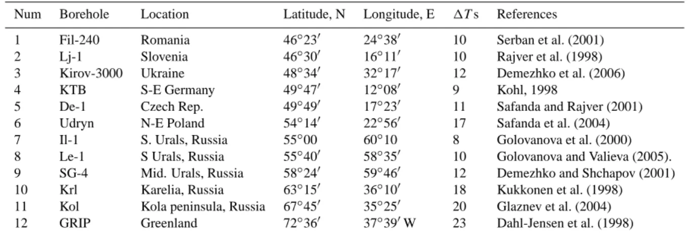
Table 1. The first group of estimates. Location of boreholes, PHW amplitude 1Ts, references.
Num Borehole Location Latitude, N Longitude, E 1T s References 1 Fil-240 Romania 46◦23′ 24◦38′ 10 Serban et al. (2001) 2 Lj-1 Slovenia 46◦30′ 16◦11′ 10 Rajver et al. (1998) 3 Kirov-3000 Ukraine 48◦34′ 32◦17′ 12 Demezhko et al. (2006) 4 KTB S-E Germany 49◦47′ 12◦08′ 9 Kohl, 1998
5 De-1 Czech Rep. 49◦49′ 17◦23′ 11 Safanda and Rajver (2001) 6 Udryn N-E Poland 54◦14′ 22◦56′ 17 Safanda et al. (2004) 7 Il-1 S. Urals, Russia 55◦00 60◦10 8 Golovanova et al. (2000) 8 Le-1 S Urals, Russia 55◦40′ 58◦35′ 10 Golovanova and Valieva (2005). 9 SG-4 Mid. Urals, Russia 58◦24′ 59◦46′ 12 Demezhko and Shchapov (2001) 10 Krl Karelia, Russia 63◦15′ 36◦10′ 18 Kukkonen et al. (1998)
11 Kol Kola peninsula, Russia 67◦45′ 35◦25′ 20 Glaznev et al. (2004) 12 GRIP Greenland 72◦36′ 37◦39′W 23 Dahl-Jensen et al. (1998)
Fig. 1. Locations of the geothermal estimates of Pleistocene-Holocene warming (PHW) amplitude. Numbers next to the esti-mates are the same as in Table 1.
Fig 2. The spatial distribution of the geothermal estimates of PHW amplitude in Northern
Fig. 2. The spatial distribution of the geothermal estimates of PHW
amplitude in Northern Eurasia (K). Solid lines represent the main pattern the distribution follows; dashed lines show local anomalies.
amplitude on the surface of the Greenland Ice Sheet. For those datasets that include a detailed ground surface tem-perature history, we estimated the PHW amplitude as the difference in average temperatures over the periods of 30–
15 thousand years before present (Late Pleistocene) and 8-0 thousand years before present (Holocene).
The second group of geothermal estimates (Table 2) char-acterizes the changes in surface temperature in the north-ern part of Westnorth-ern Siberia, and in Yakutia (Duchkov and Balobaev, 2001). In these regions, non-stationary melting of Pleistocene permafrost has a significant impact on heat transfer. The slow rate of heat transfer in permafrost allows us to neglect the time derivative term in the non-steady one-dimensional heat equation. As a result, the Stefan’s condition at the lower boundary of the permafrost may be considered an ordinary differential equation with respect to permafrost thickness
λ∂T
∂z − q0= Q dH
dt
Here, q0denotes the heat flow in the bedrock; Q is the
melt-ing heat per unit volume; H (t ) is the permafrost thickness at time t ; λ denotes thermal conductivity, which is consid-ered equal for permafrost and bedrock. The solution of the equation allows a calculation of the change in permafrost thickness, 1H, during the PHW and the associated ground surface temperature change, 1Ts(Balobaev, 1991; Duchkov and Balobaev, 2001).
3 Spatial distribution of PHW amplitude
The range of temperature change estimates – from –2 K in the lower Lena River to +23 K on the Greenland Ice Sheet – points to significant and variable changes in the surface temperature between the Pleistocene and Holocene epochs. The spatial distribution of PHW amplitudes (Fig. 2) has the following features. (1) In the Urals and west of them the amplitude increases in the northwest direction. Isoanomaly
1Ts=+10 K descends from 65◦N at the 80◦E meridian to 57◦N and 47◦N at the 60◦E and 20◦E meridians, respec-tively. East of the 80◦meridian the 1Ts=+10 K isoanomaly
D. Y. Demezhko et al.: Spatial distribution of Pleistocene/Holocene warming 561
Table 2. The second group of estimates. Location of boreholes, PHW amplitude 1T s, permafrost thickness change 1H . (Duchkov and
Balobaev, 2001).
Num Borehole Latitude, N Longitude, E 1Ts, K 1H , m
Western Siberia 1 Urengoy-1 66 79 10.4 150 2 Urengoy-2 66 79 12.3 160 3 Urengoy-3 66 80 10.3 125 4 Medvezhje-1 66 74 12.5 135 5 Medvezhje-2 66 74 12.7 170 6 Ermakovskaya 66 86 7.8 125 7 Kostrovskaya 66 86 8.8 145 8 Russkoye 67 80 9.2 100 9 Pestsovoye 67 75 10.2 120 10 Yamburg 68 75 8.7 105 11 Novy Port 68 72 2.5 35 12 Soleninskoye 69 82 5.3 45 13 Messoyakha 69 82 3.7 45 14 Arkticheskoye 70 70 0 0 15 Neytinskoye-1 70 70 4.5 35 16 Neytinskoye-2 70 70 3.5 45 17 Kharasavey 71 67 0 0 18 Kazantsevskaya 70 84 9.1 150 19 Dzhangodskaya 70 88 9.1 80 Yakutia 20 Yakutsk 62 130 8.3 218 21 Kenkeme 62 129 8 210 22 Namtsy 63 130 7.2 100 23 Orto-Surt 63 125 8 95 24 Kyz-Syr 64 124 10.3 107 25 Nedzheli 64 126 11.8 127 26 Sobo-Khaya 64 127 9.9 270 27 Balagatchi 65 124 8.6 60 28 Bakhynay 66 123 7.4 70 29 Viluisk 64 123 10.7 130 30 Promyshlenny 64 126 7.6 210 31 Govorovo 71 127 –2.3 –40 32 Dzhardzhan 68 124 13.3 50 33 Ust-Viluy 64 126 7.6 210 34 Sr.-Viluy 64 124 9.8 83 35 Oloy 63 126 9.8 140 36 Borogontsy 63 132 7.2 100
stays practically flat. Isoanomaly 1Ts=+20 K encircles Fennoscandia in the Southeast and tends northwest toward Greenland. (2) The regular pattern is violated by some of the Western Siberia and Yakutia estimates, for which the am-plitude decreases northward of 68◦N. The amplitude falls to 3–0 K at the Yamal peninsula and becomes negative, – 2 K, in the lower Lena River (i.e. here the surface tempera-ture dropped and the permafrost thickness increased by 40 m since the glaciation period, see Table 2). We believe that the origin of this deviation is unrelated to climate and that there was likely another warming factor at work for a long time.
The isoanomalies in Fig. 2 are very imprecise: for the small sample of data used, their shape depends considerably on the interpolation method. Clearly, however, the isoanoma-lies have a saturation point – a center of warming that appears to be located in the North Atlantic. The coordinates of this hypothetical center can be estimated with higher precision if one adopts a parametric mathematical model for the distribu-tion of the warming. In the present paper we do not discuss any specific mechanisms of heat transfer; instead, we test several very simple models.
Table 3. The sample of PHW amplitude estimates prepared for the
model parameters determination.
Num Table num., Num of Location 1T s, K
data num estimates
1 1: 1 1 Romania 10 2 1: 2 1 Slovenia 10 3 1: 3 1 Ukraine 12 4 1: 4,5 2 Germany, 10 Czech Rep. 5 1: 6 2 Poland 17 6 1: 7,8 1 S.Urals 9 7 1: 9 1 Mid. Urals 12 8 1: 10 1 Karelia 18 9 1: 11 1 Kola peninsula 20 10 1: 12 1 Greenland 23 11 2: 1–3,8 4 W.Siberia 10.6 12 2: 4,5,9 3 W.Siberia 11.8 13 2: 6,7 2 W.Siberia 8.3 14 2: 23–30,33–35 11 Yakutia 9.2 15 2: 20–22,36 4 Yakutia 7.7
Consider functions of the form
1Ti(ri) = k1+ k2rim, ri = r(ϕ0, λ0, ϕi, λi), (1) where ri is the distance from the center of warming with co-ordinates ϕ0 (latitude) and λ0 (longitude) to a data point i
with coordinates ϕi , λi, (i=1,2. . . n) at which the warming amplitude 1Ti is reconstructed; k1and k2are constants;
ex-ponent m=1,–1,–2 determines the functional form. Exex-ponent
m=–1 has a physical interpretation: it describes the heat flow
from a point source in a thin flat layer with the temperature anomaly 1T linear in the flux. A similar linear relationship between the outgoing heat flux and the surface temperature was proposed by Budyko (1980). The optimal model param-eters (ϕ0, λ0, k1, k2) are found by minimizing the functional
M = 1 − R2→ min (2)
where R2is the square of the linear correlation coefficient between 1T and rmfor the chosen model. Functional
M=1-R2characterizes the unexplained share of the total dispersion
D, while (DM)1/2 describes the mean square deviation of the model residuals.
To estimate the warming center position, the following adjustments have been made in the initial sample: closely located estimates have been merged, and the data north of 68◦N were removed from the sample. The adjusted sample is shown in Table 3. The estimated results for the three models are shown in Table 4. The non-linear models S2 and S3 yield the minimal values of the functional M. The mean square de-viation (DM)1/2can be regarded as an accuracy measure for the geothermal reconstruction of the Pleistocene/Holocene warming amplitude. It is below 1.5 K for the non-linear mod-els, which compares well with Dahl-Jensen et al. (1998) who
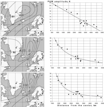
Fig 3. Isolevel surfaces of functional ( , ) (left panels), and the dependence of PHW
Fig. 3. Isolevel surfaces of functional M(ϕ0, λ0) (left panels), and
the dependence of PHW amplitude on the distance from the center of warming (right panels) for models S1–S3.
estimate the accuracy to be 2 K in their GRIP reconstruction. The differences among the nearest boreholes are also of the order of 2 K: De-1 (11 K) and KTB (9 K); Il-1 (8 K) and Le-1 (10 K), see Table 1.
Along with the optimal position of the center of warming and the value of functional M at its minimum, it is of interest to explore the shape of the minimal functional M(ϕ0, λ0) as
a function of the position. Figure 3 shows the isolevel lines of M(ϕ0, λ0) for M <0.5. Their elongated shape indicates
that the real source of warming was significantly different from a point source and looked more like a line source. The shape of this line approximately follows the pattern of warm currents in the North Atlantic. The Greenland point is most crucial in the dataset, which is spatially isolated from other estimates. If this point is eliminated from the dataset, the center of warming is shifted by 19 degrees east (Fig. 4 – red triangle). Nevertheless, even without the Greenland point, the spatial distribution of PHW amplitudes reveals asymme-try with respect to the North Pole and increases in the north-west direction. The statistical robustness of the warming cen-ter position can be tested by means of a bootstrap technique. We generated 600 subsamples with random replacement of PHW estimates (so that any data point can be sampled mul-tiple times or not sampled at all) and calculated the warming center position for each daughter subsample (for S2 model, Fig. 4 – little black circles). Most of the centers (>90%) are located in the submeridional zone that coincides with the M-functional minimum. Thus, the results suggest that dynamics
D. Y. Demezhko et al.: Spatial distribution of Pleistocene/Holocene warming 563
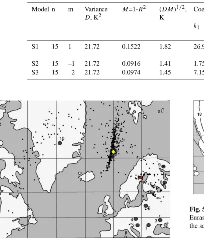
Table 4. Parameters of the model of PHW amplitude spatial distribution.
Model n m Variance
D, K2
M=1-R2 (DM)1/2, K
Coefficients Coordinates of the center
k1 k2 Latitude, N Longitude, W S1 15 1 21.72 0.1522 1.82 26.91 –4.6230 10−3 74.94◦ 12.32◦ S2 15 –1 21.72 0.0916 1.41 1.75 2.7141 104 71.12◦ 0.31◦ S3 15 –2 21.72 0.0974 1.45 7.15 2.9999 104 69.05◦ 0.80◦
Fig. 4. Bootstrapping the data. Yellow rhombus – PHW warming
center position for the initial sample; red triangle – the same for the sample with eliminated Greenland estimate; little black circles – PHW warming center position for the randomly generated sub-samples.
in the North Atlantic region could be a source of the PHW. Sufficiently far from the source, e.g., in Yakutia, the warming amplitude drops to 7–9 K. Here, most likely, the warming is not directly related to changes in the Atlantic, but determined by the reaction of the planetary climate system to the initial regional warming.
The results of our modeling can also be useful for tradi-tional geothermal problems, in particular, for finding paleo-climatic corrections to the measured heat flow density. The PHW distorts the heat flow for depths of up to ∼2.5 km. For depths up to ∼500 m this distortion is complemented by Holocene climate changes. Therefore, the distribution of PHW amplitudes shown in Fig. 5 can be used to calculate the paleoclimatic corrections in the interval 500–2500 m. This dependence may be disturbed at coastal regions or in the ar-eas covered by glaciers in the Late Pleistocene (we discuss the reasons of this below). Using the obtained dependence for paleoclimatic corrections in these areas should be con-sidered as unreliable.
Fig 5. The spatial distribution of PHW amplitudes (K) in Northern Eurasia Fig. 5. The spatial distribution of PHW amplitudes (K) in Northern
Eurasia according the model S2. Numbers next to the estimates are the same as in Table 3.
4 Deviation from the regular pattern
A number of geothermal PHW estimates for Western Siberia and Yakutia deviate significantly from the regular pattern identified (Fig. 2). The anomalously low PHW values are lo-calized spatially and can be reliably identified (see the dashed 10 K lines in Fig. 2) even after we take noise into account. The warming amplitudes decrease to 3–0 K at the Yamal Penisula and to –2 K in the lower Lena River. Thus, the Late Pleistocene surface temperatures in these regions were only slightly below and, in some cases, even above the tem-perature today. This observation points to the existence of a warming source that was affecting the surface for a long time.
One possible source of the warming effect is the influ-ence of Late Pleistocene ice sheets. According to the Panar-ctic Ice Sheet hypothesis (Hughes et al., 1977; Grosswald, 1996), Arctic Eurasia was covered by a continuous chain of glaciers during the Late Pleistocene. The Kara’s and East-Siberian Ice Sheets were part of this region (Fig. 6 – blue area). According to another hypothesis of limited Pleistocene glaciation (Velichko, 2002) there was no continental Late Pleistocene glaciation in Western Siberia and Yakutia (Fig. 6 – brown areas). However, the following question arises: if the influence of speculated Siberian glaciers can be so easily
Fig. 6. Late Pleistocene Ice Sheets in Northern Eurasia. Blue area
– according to the Panarctic Ice Sheet hypothesis (Hughes et al., 1977, Grosswald, 1996): Sc – Scandinavian, K – Kara’s, ES – East Siberian. Brown areas – according to the limited Pleistocene glacia-tion hypothesis (Velichko, 2002).
traced in today’s temperature field, why is there no similar trace of the well-established Scandinavian Ice Sheet? The unexpectedly high geothermal estimates of PHW amplitudes for holes on the Kola peninsula (Kol, 1T =20 K, Glaznev et al., 2004), in Karelia (Krl, 1T =18 K, Kukkonen et al.,1998), and in Poland (Udryn, 1T =17 K, Safanda et al., 2004) con-tain no indication of glacier-related warming.
It should be mentioned here that we have not included in our analysis some estimates from the vicinity of the Kola super-deep borehole (Rath and Mottaghy, 2006) and from Outokumpu, Finland (Kukkonen and Safanda, 1996), which show moderate PHW amplitudes of about 4–7 K. The ampli-tudes of reconstructed climatic events in the first case may be essentially suppressed by the Tikhonov’s regularization - the higher the regularization parameter the smoother the objec-tive function. The result from Outokumpu may be also irrel-evant as it was obtained for shallow boreholes (790–1100 m) and under 2-D heat transfer conditions. Our analysis shows that insufficient depths may lead to underestimation of pa-leotemperature changes (Golovanova et al., 2002; this effect was also mentioned in Majorowicz et al., 2002, 2006). How-ever, it must not be ruled out that comparatively low PHW amplitudes in these sites reflect the spatial temperature vari-ations at the base of the Scandinavian Ice Sheet. In fact, a glacier’s influence on the ground surface temperature is complex. Several factors contribute to changes in the tem-perature under a glacier: geothermal heat flow and friction lead to temperature increases, while vertical ice flow leads to decreases. Surface temperature changes, in turn, affect me-chanical properties of the ice. Numerical model simulations (Payne et al., 2000) show that an interplay of all these factors may lead to a thermomechanical instability, which makes it impossible to predict the basal temperature distribution.
We estimated the influence of the glacier on ground sur-face temperatures using a simple one-dimensional stationary model, which also takes into account the role of snow cover,
an additional factor that we believe to be significant. With-out a glacier, the mean annual ground surface temperature is determined by the air temperature and the warming influ-ence of snow cover. This warming influinflu-ence increases with the snow cover height and with the amplitude of the seasonal air temperature variation, and decreases with the increasing mean annual air temperature (Demezhko, 2001). The glacier eliminates this effect and somewhat cools the ground surface. Consider heat transfer in an instantly emerged glacier of a finite height h, which covers a semi-infinite massif of bedrock. Let the thermal properties of the ice and the rock be constant but different. Further, let the velocity of the vertical ice flow at the glacier surface be equal to the accumulation rate, and hence the height h is constant. With the vertical axis
z directed downward and the origin at the flat impenetrable
ice/rock contact surface, the system of one-dimensional heat equations can be written in the form
∂2T i ∂z2 − Viz(z) ai ∂Ti ∂z = 1 ai ∂Ti ∂t , −h ≤ z ≤ 0 ∂2T0 ∂z2 = 1 a0 ∂T0 ∂t , z > 0 Viz(z) = −Vsz/ h. (3)
Here, subscripts i and 0 refer to the glacier and the rock, re-spectively; a denotes thermal diffusivity; Viz(z) is the verti-cal component of the ice flow velocity that linearly decreases with depth from its maximal value Vsat the glacier surface to zero at the ice/rock boundary. The flow velocity at the glacier surface, Vs=Viz(−h), coincides with the accumulation rate. We assume that the temperature at the glacier surface, Tis, and the geothermal heat flow, q0, are independent of time,
Ti(−h, t) = Tis,
λ0∂T∂z0 = q0 for z → ∞
, (4)
and that the temperatures and heat flows in the two media are equal to each other at the ice/rock contact surface,
Ti(z, t ) = T0(z, t )andλi
∂Ti
∂z=λ0 ∂T0
∂z at z=0. (5)
For times significantly exceeding the penetration time of the fastest “temperature signal” in the glacier,
t >>min(h/Vs, h2/4ai), the temperature distribution will become stationary everywhere:
Tist(z) = Tis+ G0hλλ0 i √ π 2 erf (√P em)+erf (√P em(z/ h)) √ P em T0st(z) = Tis+ G0hλλ0 i √ π 2 erf (√√P em) P em + G0z, (6)
Here, erf(u) is the error function, λ denotes thermal conduc-tivity, G0= q0/λ0is the geothermal gradient in the rocks
cor-responding to the geothermal heat flow q0; Pem = Vimh/ai is the ice Peclet number determined by the average flow ve-locity in the glacier Vim= Vs/2.
We tested the model using modern data on the temperature distribution, ice height, accumulation rates and surface tem-perature of the Greenland Ice Sheet (http://www.nsidc.org/
D. Y. Demezhko et al.: Spatial distribution of Pleistocene/Holocene warming 565
Fig. 7. Comparison of measured (blue) and calculated (dashed red)
temperature-depth profiles in the Greenland Ice Sheet. Measured data were taken from (Dahl-Jensen et al., 1998 – Dye-3) and (GRIP Temperature Profile: http://www.nsidc.org/data/gispgrip/data/grip/ physical/griptemp.dat, access: 12 July 2001).
data/gisp grip/data/grip/physical/griptemp.dat, Dahl-Jensen et al., 1998). Figure 7 shows the comparison between mea-sured and calculated (according to the model) temperature-depth profiles in the Greenland Ice Sheet. Here we used the following initial conditions: the accumulation rate (equal to the vertical ice flow velocity) at the glacier surface is 0.23 (GRIP) and 0.49 (Dye) m/year (Dahl-Jensen et al, 1998); thermal conductivity of the ice is 2.17–2.23 W m−1K−1; geothermal gradient in the base of the glacier is 0.027 (GRIP) and 0.013 (Dye) K/m; vertical air temperature gradient is 0.006 K/m; and ice sheet thickness is 3029 m (GRIP) and 2037 m (Dye-3). The model yields vertical temperature vari-ations that agree well with the temperature-depth profiles. The difference between the calculated and real GRIP profiles between approximately –3000 to –1500 m is due to paleocli-matic changes. The glacier near Dye-3 has lower thickness,
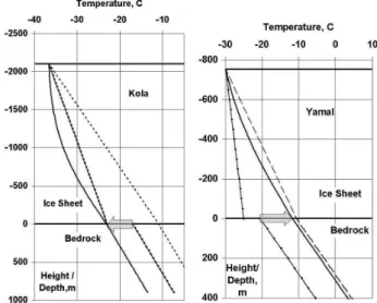
Fig. 8. The Influence of Late Pleistocene ice sheets on the basal
temperature. The solid lines with points show the initial tempera-ture distribution; the dashed lines show the stationary temperatempera-ture distribution with no vertical ice advection; the solid lines show the stationary temperature distribution with vertical ice advection.
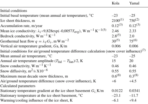
while the vertical ice flow is larger; therefore, here the pa-leoclimatic anomaly (mainly from the PHW) is “smeared” towards larger depths, including the rock. Extrapolation of the modern glacier surface temperature (–35.1◦C for GRIP and –20.3◦C for Dye-3) with the vertical air temperature gra-dient 0.006 K/m on the bedrock surface, gives the hypotheti-cal bedrock surface temperature without the glacier (–16.9◦C for GRIP and –8.1◦C for Dye-3). Observed temperatures at the base of the glacier are –8.4◦C for GRIP and –13.2◦C for Dye-3. Thus, near GRIP the glacier warms up the rock by 8.5 K, while near Dye-3 it cools the rock down by 5.1 K due to a higher ice flow velocity. As a result, the basal tempera-ture near GRIP is 4.8 K higher than that near Dye-3, though GRIP is situated 800 km farther north. Thus, the presence of a glacier does not necessarily lead to a temperature in-crease at its base: a fast enough vertical ice flow can transfer low temperatures down from the outer surface. We calcu-lated the warming influence of the Scandinavian and Kara’s Ice Sheets for two regions: the Kola Peninsula (near the Kol hole, 67.8◦N) and the Yamal Peninsula (near the holes Arc-tic, Nejtinsk-1 and Nejtinsk-2, 70◦N). We used the initial pa-rameters of the ice cover (thickness and accumulation rates) obtained within the QUEEN initiative (Quaternary Environ-ment of the Eurasian North, Hubberten et al., 2004), which combined a number of numerical experiments and indirect paleoclimatic data sources. The initial data and our results are shown in Fig. 8 and Table 5.
The warming influence of the glacier was calculated rel-ative to the average temperature of the upper layer of the rocks, which exceeds the surface air temperature due to the warming influence of snow cover. Low heat flow on the Kola
Table 5. Initial conditions and calculated ice-sheet temperatures.
Kola Yamal Initial conditions
Initial basal temperature (mean annual air temperature),◦C –23 –25 Ice sheet thickness, m 2100(1) 750(2) Accumulation rate, m/year 0.12(3) 0.12(3) Mean ice conductivity: λi=9,828exp(–0,0057Tavg), W m−1K−1(5) 2.46 2.33
Bedrock conductivity, W m−1K−1 2.8(5) 2.0 Geothermal heat flow q = λIGi, m W m−2 30(5) 75(6)
Vertical air temperature gradient, Ga, K/m 0.006 0.006 Initial conditions for air/ground temperature difference calculation (snow cover influence)(7) Mean annual air temperature,◦C –23 –25 Annual air temperature amplitude (TJul− TJan)/2, K 15 20 Snow conductivity, W m−1K−1 0.46 0.46 Snow diffusivity, m2/s X10−6 0.55 0.55 Maximum mean decade snow thickness, m 0.6(8) 0.3(8) Air/ground temperature difference (snow cover influence), K +6 +4.5 Calculated parameters
Stationary temperature gradient at the ice sheet basement Gi,K/m 0.0122 0.0341 Stationary temperature at the ice sheet basement,◦C –23.1 –11.7 Warming/cooling influence of the ice sheet, K –6.1 +9.4
Comments:
(1)The maximal value of the ice sheet thickness obtained from the models ISM (Siegert et al., 2001) and AGCM (Hubberten et al., 2004)
was used.
(2)From the model AGCM (Hubberten et al., 2004).
(3)The minimal value of the accumulation rate from the model AGCM (Hubberten et al., 2004). (4)Tarasov and Peltier (2003)
(5)Glaznev et al. (2004)
(6)Temperature, permafrost. . . , (1994).
(7)The algorithm proposed by Demezhko (2001).
(8)Contemporary values of maximum mean decade snow thickness were used.
Peninsula (30 mW/m2) causes cooling of the upper layer of
the rocks by 6.1 K, even though the accumulation rate is low, 0.12 m/year. On Yamal, with the same accumulation rate but a heat flow of 75 mW/m2, the base of the glacier could warm up by 9.4 K. Although this number is close to the deviations of the PHW amplitude in the holes Arctic, Nejtinsk-1 and Nejtinsk-2 from the global distribution (12.8, 8.3 and 9.3 K, respectively), it hardly proves that the deviation from the reg-ular pattern in the PHW amplitude distribution at the Arctic coast of Western Siberia is related exclusively to the warming influence of the Kara’s Ice Sheet. The temperature changes caused by the glacier could leave a significant trace in the modern temperature field only if they persisted for several tens of thousands of years – a period comparable to the time elapsed after the decay of the glacier. Besides, several tens of thousands of years are needed to reach stationary condi-tions. At the same time, modern data show that the Kara’s Ice Sheet was most developed during the Early and Middle Weichselian (90–60 thousand years before present), and its decay occurred at the peak of the last glaciation period
(Kara-banov et al., 1998; Saarnisto, 2001; Velichko, 2002). The “glacier hypothesis” is even less convincing at explaining the Late Pleistocene warming in the lower Lena River. Most researchers agree that there was no developed Pleistocene glaciation in that region. We therefore further explore an ex-planation for the deviations from the observed PHW patterns in the Discussion and Conclusion section of this manuscript.
5 Discussion and conclusion
Our main conclusion is that information extracted from geothermal data is a sufficiently reliable and new data source that is independent from the existing set of paleoclimatic in-dicators. The climate system of the Earth will be understood better if all such indicators, including the geothermal ones, are jointly taken into account. We have used the geother-mal data to identify two features in the spatial distribution of Pleistocene/Holocene warming amplitudes: (i) The ampli-tudes increase in the northwest direction; and (ii) The latitude
D. Y. Demezhko et al.: Spatial distribution of Pleistocene/Holocene warming 567 dependence of the estimates in Western Siberia and Yakutia
north of the 68-th parallel exhibits inversion.
The first, and major, feature could be described by a model that assumes that the warming was spreading from a hypo-thetical center with an amplitude that is a nonlinear func-tion of the distance from the center. According to the model there exists a warming source (most likely an extended line source) located northeast of Iceland. An alternative to this simple model could be a more complex parametric model, or a detailed non-parametric analysis, both of which are not possible presently due to the small sample size. We believe that the model we have chosen is the simplest possible model that is still adequate given the quality and the quantity of the available data. High explanatory power of the model (the un-explained share of the total variance in model S2 is only 9%) also speaks in its favor.
The elongated shape of the PHW source follows the pat-tern of warm currents in the North Atlantic. In the Late Pleis-tocene there was no such anomaly, and probably no Gulf-stream, North-Atlantic and Norwegian currents causing it, at least in their modern form. Our geothermal inference sup-ports the famous idea of a key role played by the North At-lantic currents in the development of the ice ages (see Stew-art, 2006). Nevertheless, we cannot exclude other warming mechanisms that might explain the distribution of PHW am-plitudes. For instance, Seager et al. (2002) proposed that the principal cause of the temperature anomaly is advection by the mean winds.
Our second finding – the inversion of the latitude depen-dence of the estimates in Western Siberia and Yakutia north of the 68-th parallel - is also quite remarkable. The low esti-mates of PHW amplitudes for Arctic Siberia point to the exis-tence of a non-climatic warming factor, the origin of which is not entirely clear. The relevant source of warming should be more powerful than the geothermal heat flow, and its duration longer than the lifetime of the ice sheets. One such source could be explained by the hypothesis of Karnaukhov (1994), according to which giant ice dams were formed in the mouths of the Ob, Yenisey and Lena Rivers during the ice ages. The ice broke up on these rivers in the South and accumulated in their mouths in the North forming the dams. The dams interrupted drainage and large regions were flooded. The warming effect of this must have been significant because the flood water was already warmed in the South. Similar but smaller-scale dams and floods occur now as well, their du-ration and scale increasing when the temperature drops and the latitude gradient of the mean annual temperature rises. Ice-damming of lakes is mentioned also in the Panarctic Ice Sheet model (Hughes et al., 1977; Grosswald, 1996). In both hypotheses, a large-scale flooding of entire Western-Siberian lowlands was assumed. This could indeed be the case, but only during a relatively short (in the geothermal sense) pe-riod of time – less than 10 thousand years. As for the pepe-riod comparable to the duration of an ice age, about 70 thousand years, the flooding (continuous or periodic) only occurred in
a small region within the identified anomalies of geothermal estimates, i.e. north of the 68-th parallel.
Acknowledgements. We are grateful to J. Smerdon for his
con-structive suggestions and improvements of the text, as well as to J. Safanda, and two anonymous reviewers for their critical com-ments. This research was financially supported by the Integrated Project between the Ural and Siberian Branches of the RAS, “Reconstruction of the spatial distribution of Pleistocene-Holocene warming amplitudes in Northern Eurasia by geothermal data” and RFBR grant 06-05-64084.
Edited by: J. Smerdon
References
Balobaev, V. T.: Geothermics of permafrost zone of the lithosphere of Northern Asia. Novosibirsk, Nauka, 194 pp., (in Russian), 1991.
Budyko, M. I.: Climate in the past and future. Leningrad, Gidrom-eteoizdat, 352 pp. (in Russian), 1980.
Dahl-Jensen, D., Mosegaard, K., Gundestrup, N., Clow, G. D., Johnsen, S. J., Hansen, A. W., and Balling, N.: Past temperature directly from the Greenland ice sheet, Science, 282, 268–271, 1998.
Demezhko, D. Y. and Shchapov, V. A.: 80 000 years ground sur-face temperature history inferred from the temperature-depth log measured in the superdeep hole SG-4 (the Urals, Russia), Global and Planetary Change, 29(3–4), 219–230, 2001.
Demezhko, D. Y.: Geothermal method for paleoclimate reconstruc-tion (examples from the Urals, Russia), Russian Academy of Sci-ence, Ekaterinburg: Urals Branch, 143 pp. (in Russian), 2001. Demezhko, D. Y., Utkin, V. I., Shchapov, V. A., and Golovanova, I.
V.: Variations in the Earth’s Surface Temperature in the Urals during the Last Millennium Based on Borehole Temperature Data, Doklady Earth Sciences, 403(5), 764–766, 2005.
Demezhko, D. Y., Utkin, V. I., Duchkov, A. D., and Ryvkin, D. G.: Geothermic Estimates of the Amplitudes of Holocene Warming in Europe, Doklady Earth Sciences, 407(2), 259-261, 2006. Duchkov, A. D. and Balobaev, V. T.: Evolution of a thermal and
phase condition of Siberian permafrost, in: Global changes of the natural environment – 2001, edited by: Dobretsov, E. L. and Ko-valenko, V. I., Novosibirsk, Publishing house SB RAS, Branch “GEO”, 79–104 (In Russian), 2001.
Velichko, A. A. (Ed.): Dynamics of terrestrial landscape compo-nents and inner marine basins of the Northern Eurasia during the last 130 000 years, Atlas-monograph, GEOS, Moscow, 296 pp. (in Russian), 2002.
Glaznev, V. N., Kukkonen, I. T., Raevskii, A. B., and Jokinen, J.: New Data on Thermal Flow in the Central Part of the Kola Peninsula. Transactions (Doklady) of the Russian Academy of Sciences, Earth Science Section, 2004, 396(4), 512–514, 2004. Golovanova, I. V., Selezneva, G. V., and Smorodov, E. A.:
Recon-struction of the warming after glaciation in the South Urals by the temperature measurements in boreholes, Geologitheskiy sbornik, 1, IG UB RAS, Ufa, 113–116 (in Russian), 2000.
Golovanova, I. V., Demezhko, D. Y., Shchapov, V. A., and Se-lezniova, G. V.: Paleoclimatic analysis of geothermal data. Dif-ferent approaches (II). Proceedings of the Int. Conf. “The Earth’s
thermal field and related research methods”, Moscow, 79–81, 2002.
Golovanova, I. V. and Valieva, R. Y.: New estimates of paleoclimate change in the South Urals by the geothermal data, Proceedings of the III-d Scientific Readings in Memory of Yu.P.Bulashevich, Ekaterinburg. IGF UB RAS, 86–87 (in Russian), 2005. Grosswald, M. G.: Evidence for a glacial invasion of the
East Siberian coasts from the adjacent Arctic shelf, Doklady Akademii Nauk., 350(4), 535–540, 1996.
Huang, S., Pollack, H. N., and Shen, P. Y.: Late Quaternary temper-ature changes seen in world-wide continental heat flow measure-ments, Geophys. Res. Lett., 24, 1947–1950, 1997.
Hubberten, H., Andreev, A., Astakhov, V., et al.: The periglacial climate and environment in northern Eurasia during the Last Glaciation, Quaternary Science Reviews 23, 1333–1357, 2004. Hughes, T. J., Denton, G. H., and Grosswald, M. G.: Was there a
late W¨urm Arctic Ice Sheet?, Nature, 266, 596–602, 1977. Karabanov, E., Prokopenko, A/, Williams, D., and Colman, S.:
Ev-idence from Lake Baikal for Siberian Glaciation during Oxygen-Isotobe Substage 5d, Quart. Res., 50, 46–55, 1998.
Karnaukhov, A. V.: Dynamics of glaciations in Northern Hemi-sphere as the process of self-oscillation and relaxation, Bio-physics, 39(6), 1094–1098 (in Russian), 1994.
Kohl, T.: Palaeoclimatic temperature signals – can they be washed out?, Tectonophysics, 291, 225–234, 1998.
Kukkonen, I. T. and Safanda, J.: Palaeoclimate and structure: the most important factors controlling subsurface temperatures in crystalline rocks. A case study from Outokumpu, eastern Fin-land’, Geophys. J. Int. 126, 101–112, 1996.
Kukkonen, I. T., Gosnold, W. D., and ˇSafanda, J.: Anomalously low heat flow density in eastern Karelia, baltic Shield: a possible paleoclimate signature, Tectonophysics 291, 235–249, 1998. Kukkonen, I. T. and Joeleht, A.: Weichselian temperatures from
geothermal heat flow data, J. Geophys. Res., 108(B3), 2163, doi:10.1029/2001JB001579, 2003.
Majorowicz, J., Safanda, J., and Scinner, W.: East to west retar-dation in the onset of the recent warming across Canada inferred from inversions of temperature logs, J. Geophys. Res., 107(B10), 2227, doi:10.1029/2001JB000519, 2002.
Majorowicz, J., Grasby, S. E., Ferguson, G., Safanda, J., and Skin-ner, W.: Paleoclimatic reconstructions in western Canada from borehole temperature logs: surface air temperature forcing and groundwater flow, Clim. Past, 2, 1–10, 2006,
http://www.clim-past.net/2/1/2006/.
Payne, A. J., Huydrechts, P., Abe-Ouchi, A., et al.: Results from EISMINT model intercomparison: the effects of thermomechan-ical coupling, J. Glaciology, 46(153), 227–238, 2000.
Pollack, H. N., Hurter, S. J., and Johnson, J. R.: Heat flow from the Earth’s interior: Analysis of the global data set, Rev. Geophys., 31, 267–280, 1993.
Rath, V. and Mottaghy, D.: Paleoclimate on the Kola Peninsula (Russia) from inversion of subsurface temperatures, Geophys. Res. Abstr., 7, 03224, 2005.
Rajver, D., Safanda, J., and Shen, P. Y.: The climate record inverted from borehole temperatures in Slovenia, Tectonophysics, 291, 263–276, 1998.
Saarnisto, M.: Climate variability during the last interglacial-glacial cycle in NW Eurasia. /PAGES - PEPIII: Past Climate Variabil-ity Through Europe and Africa, August 27–31, Aix-en-Provence, France, (http://atlas-conferences.com/c/a/h/i/79.htm), 2001. Safanda, J. and Rajver, D.: Signature of the last ice age in
the present subsurface temperatures in the Czech Republic and Slovenia, Global Planet Change, 29(3–4), 241–258, 2001. Safanda, J., Szewczyk, J., and Majorowicz, J.: Geothermal
evidence of very low glacial temperatures on a rim of the Fennoscandian ice sheet, Geophys. Res. Lett., 31, L07211, doi:10.1029/2004GL019547, 2004.
Seager, R., Battisti, D. S., Yin, J., Gordon, N., Naik, N., Clement, A. C., and Cane, M. A.: Is the Gulf Stream responsible for Europe’s mild winters?, Quart. J. Royal Meteorol. Soc., 128, 2563–2586, 2002.
Serban, D. Z., Nielsen, S. B., and Demetrescu, C.: Long wavelength ground surface temperature history from continuous temperature logs in the Transilvanian Basin, Global Planet Change, 29(3–4), 201–218, 2001.
Siegert, M. J., Dowdeswell, J. A., Hald, M., and Svendsen, J.-I.: Modelling the Eurasian Ice Sheet through a full (Weichselian) glacial cycle, Global Planet. Change, 31, 367–385, 2001. Stewart, R. H.: Introduction to Physical Oceanography.
On-line textbook, 2006 (http://oceanworld.tamu.edu/resources/ ocng textbook/PDF files/book pdf files.html).
Tarasov, L. and Peltier, W. R.: Greenland glacial history, borehole constraints, and Eemian extent, J. Geophys. Res., 108(B3), 2143, doi:10.1029/2001JB001731, 2003.
Duchkov, A. D., Balobaev, V. T., Volodko, B. V., et al.: Temper-ature, permafrost and radiogenic heat production in the Earth’s crust of Northern Asia, UIGGM SB RAS, Novosibirsk, 141 pp. (in Russian), 1994.