Supporting information
S1 TextLinear stability analysis
We performed some further analysis to differentiate the four prototypical models by exposing their steady states and related stability properties, following a classical method (Murray, 2011). These structural properties show that the first two models (activating and inhibiting) exhibit similar behaviors, while the two mixed situations possess very different features. Recall that the systems of interest are given by equations (1-3) in the Main Text, which have the following form,
{ 𝜕𝐴(𝑡,𝑥) 𝜕𝑡 = 𝐹𝐴(𝐴, 𝐼, 𝑆) + 𝐷𝑎∇ 2 𝐴 𝜕𝐼(𝑡,𝑥) 𝜕𝑡 = 𝐹𝐼(𝐴, 𝐼, 𝑆) + 𝐷𝑖∇ 2 𝐼 𝜕𝑆(𝑡,𝑥) 𝜕𝑡 = 𝐹𝑆(𝐴, 𝐼, 𝑆) (S1)
Diffusive-driven instability occurs when a steady state, linearly stable in the absence of diffusion, turns unstable, if diffusion is present. First, the eigenvalues of the Jacobian 𝐽(𝐴, 𝐼, 𝑆) of the system at steady state are studied in absence of diffusion. The Jacobian is the matrix of the partial derivatives of 𝐹𝐴, 𝐹𝐼, and 𝐹𝑆 with respect to the state variables 𝐴, 𝐼, and 𝑆. In other words,
𝐽(𝐴, 𝐼, 𝑆) = ( 𝜕𝐹𝐴 𝜕𝐴 𝜕𝐹𝐴 𝜕𝐼 𝜕𝐹𝐴 𝜕𝑆 𝜕𝐹𝐼 𝜕𝐴 𝜕𝐹𝐼 𝜕𝐼 𝜕𝐹𝐼 𝜕𝑆 𝜕𝐹𝑆 𝜕𝐴 𝜕𝐹𝑆 𝜕𝐼 𝜕𝐹𝑆 𝜕𝑆 )
Where partial derivatives are evaluated at (𝐴, 𝐼, 𝑆). A fixed point (steady state) of the system (S1) with no diffusion is called linearly stable, if all real parts of the eigenvalues of 𝐽(𝐴𝑠, 𝐼𝑠, 𝑆𝑠) are strictly
negative. For simplicity, we assume here that 𝑟𝑣(𝑡) ≡ 1 and that 𝑑𝑎= 𝑑𝑖 = 𝑑𝑠= 𝑑 > 0. Moreover,
we consider 𝜎𝑎2= 𝜎𝑖2= 0, i.e. there is no stochastic process in the system. We are interested in
steady states. From equation (3), we set
0 = 𝑑𝑆(𝑡, 𝑥)
𝑑𝑡 = 𝑟𝑣(𝑡) ∙ (𝑏𝑠
(𝐴/𝐼)2
𝐾 + (𝐴/𝐼)2 − 𝑑𝑠 𝑆(𝑡, 𝑥) + 𝑟𝑝 ).
Since 𝑟𝑣(𝑡) > 0 for all 𝑡, this leads to
𝑆𝑠= 𝑏𝑠 𝑑 ∙ (𝐴𝑠/𝐼𝑠)2 𝐾 + (𝐴𝑠/𝐼𝑠)2 +𝑟𝑝 𝑑
To simplify notations, we do not write explicitly the dependence of 𝑆𝑠, 𝐴𝑠, and 𝐼𝑠 on 𝑥.
I) Activating situation. Recall that in this case we use 𝑓(𝑠) = 𝑔(𝑠) = 𝑠. As such, the system to
be solved at steady state is the following
{𝑏𝑏𝑎𝑆𝑠− 𝑑 𝐴𝑠 = 0
𝑖𝑆𝑠− 𝑑 𝐼𝑠= 0
Plugging 𝑆𝑠 into this system of equations leads to the following unique fixed-point solution, i.e. the
system has only one single steady state:
𝐴𝑠 = 𝑏𝑎 𝑑 𝑆𝑠, 𝐼𝑠= 𝑏𝑖 𝑑𝑆𝑠, 𝑆𝑠= 𝑏𝑖2 𝐾 𝑟𝑝+ 𝑏𝑎2∙ (𝑏𝑠+ 𝑟𝑝) 𝑑 ∙ (𝑏𝑖2 𝐾 + 𝑏 𝑎2)
Now, we compute the Jacobian of the system, taking the partial derivative of the system’s equations (1-3) from the Main Text, which is given by
𝐽(𝐴, 𝐼, 𝑆) = ( −𝑑 0 𝑏𝑎 0 −𝑑 𝑏𝑖 2𝑏𝑠𝐾 (𝐴𝑠2+ 𝐼𝑠2𝐾)2 𝐴𝑠𝐼𝑠2 − 2𝑏𝑠𝐾 (𝐴2𝑠+ 𝐼𝑠2𝐾)2 𝐴𝑠2𝐼𝑠 −𝑑 )
and whose eigenvalues (𝜆1, 𝜆2, and 𝜆3) at the fixed point (𝐴𝑠, 𝐼𝑠, 𝑆𝑠) are all equal and given by
𝜆1= 𝜆2= 𝜆3= −𝑑 < 0.
As such the system’s steady state is linearly stable. It has been computed with the software Mathematica 10 (Wolfram Research, USA).
Now, we go one step further and ask about diffusion-driven instability, as originally done by Turing in the study of his reaction-diffusion system (Turing, 1952). The basic idea is that adding diffusion in the system can produce a sufficient disturbance to generate patterns. To do so, consider the system (S1) with diffusion terms and linearized around the steady state. This problem is equivalent to the following eigenvalues/eigenfunctions problem (see Chapter 2 in Murray’s book (Murray, 2011), for all details) 𝜆 𝑊𝑘 = 𝐽(𝐴𝑠, 𝐼𝑠, 𝑆𝑠) 𝑊𝑘− ( 𝐷𝑎 0 0 0 𝐷𝑖 0 0 0 0 ) 𝑘2 𝑊𝑘,
where 𝑊𝑘 is the eigenfunction, 𝜆 the eigenvalue, and 𝑘 is the wave number. This is thus equivalent
to study the eigenvalues of the following matrix,
𝐽∗(𝐴𝑠, 𝐼𝑠, 𝑆𝑠) = 𝐽(𝐴𝑠, 𝐼𝑠, 𝑆𝑠) − (
𝐷𝑎 𝑘2 0 0
0 𝐷𝑖 𝑘2 0
0 0 0
),
And find some 𝑘, so that at least one eigenvalue has a positive real part, leading to diffusion-driven instability. To do so, we will apply the Routh-Hurwitz test (See in the book entitled “An Introduction to Mathematical Biology Chapter 4.5 (Allen, 2007)). In our case, the characteristic polynomial 𝑝(𝜆) is of degree three,
𝑝(𝜆) = 𝑎3𝜆3+ 𝑎2𝜆2+ 𝑎1𝜆 + 𝑎0
Since we are interested in its roots, i.e. 𝑝(𝜆) = 0, we can normalize it so that 𝑎3= 1. In this case,
the Routh-Hurwitz test states that the roots of 𝑝(𝜆) have all negative real parts, if and only if 𝑎2> 0,
𝑎0> 0, and 𝑎2𝑎1> 𝑎0. For our problem, it thus suffices to find one condition that is not satisfied.
After normalization, the coefficients are as follows,
𝑎2= 3𝑑 + (𝐷𝑎+ 𝐷𝑖) 𝑘2> 0
𝑎1= 3𝑑2+ 2𝑑(𝐷𝑎+ 𝐷𝑖) 𝑘2+ 𝐷𝑎𝐷𝑖𝑘4> 0
𝑎0= 𝑑3+ (𝑑2(𝐷𝑎+ 𝐷𝑖) − 𝜒(𝐷𝑖− 𝐷𝑎)) 𝑘2+ 𝑑𝐷𝑎𝐷𝑖 𝑘4
Where we define for convenience the positive quantity
𝜒 = 2𝑏𝑎
2𝑏
𝑖2𝑏𝑠𝑑2𝐾
(𝐴𝑠2+ 𝐼
𝑠2𝐾)2∙ (𝑏𝑖2𝐾𝑟𝑝+ 𝑏𝑎2∙ (𝑏𝑠+ 𝑟𝑝))
The coefficients 𝑎1 and 𝑎2 are positive with our assumptions (all parameters in the system are
positive). However, 𝑎0(𝑞) is a quadratic function in 𝑞 = 𝑘2. It is convex since 𝑑𝐷𝑎𝐷𝑖 > 0. There
exists thus some 𝑘2 such that 𝑎0 is negative whenever 𝑎0(𝑞) possesses two roots. This is the case, if
the discriminant is positive, i.e. our (sufficient) condition for diffusion-driven instability is as follows, (𝑑2(𝐷𝑎+ 𝐷𝑖) − 𝜒(𝐷𝑖− 𝐷𝑎))
2
− 4𝑑𝐷𝑎𝐷𝑖> 0
and the roots of 𝑎0(𝑞) are positive (since they are of the form 𝑘2). Knowing that 𝑎0(0) > 0 and that
𝑎0 is a parabola, we can, for example, impose that 𝑎0′(0) < 0. Our sufficient condition for
diffusion-driven instability is thus
(𝑑2(𝐷𝑎+ 𝐷𝑖) + 𝜒(𝐷𝑎− 𝐷𝑖)) 2 − 4𝑑𝐷𝑎𝐷𝑖 > 0 with 𝑑2(𝐷 𝑎+ 𝐷𝑖) + 𝜒(𝐷𝑎− 𝐷𝑖) < 0.
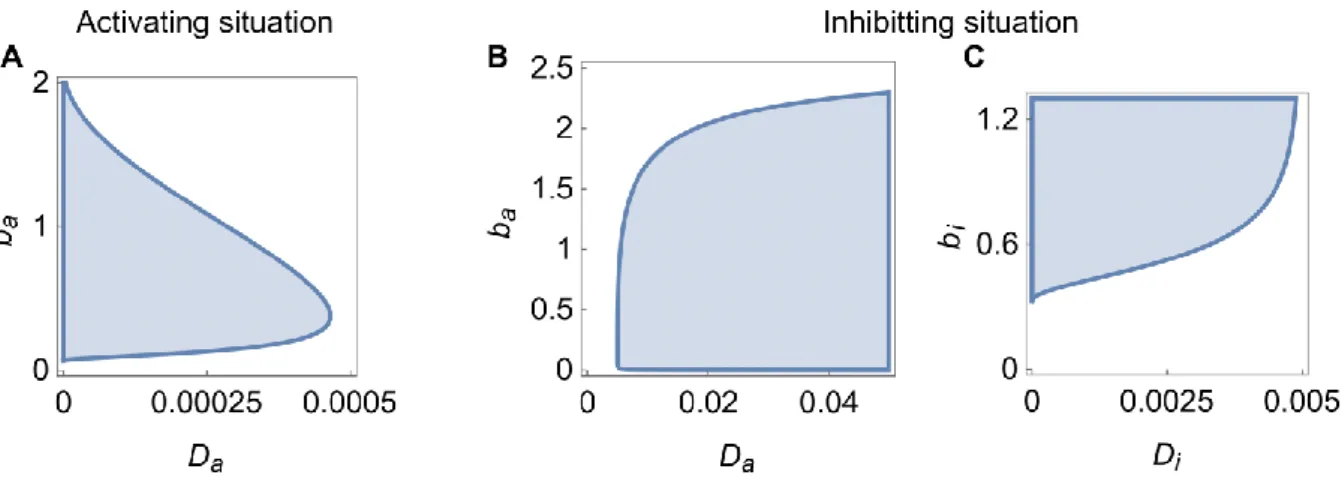
Note that this last condition implies 𝐷𝑎< 𝐷𝑖. More precisely, 𝐷𝑎< 𝐷𝑖 𝜒−𝑑2
𝜒+𝑑2. We plotted this
condition for diffusion-driven instability in Fig. S1A as a function of the parameters 𝑏𝑎 and 𝐷𝑎 (all
other parameters as in Fig. 2A-C from the Main Text).
II) Inhibiting situation. Recall that in this case we use 𝑓(𝑠) = 𝑔(𝑠) = 1/𝑠. As such, the system to be
solved at steady state is as follow
{ 𝑏𝑎 1 𝑆𝑠 − 𝑑 𝐴𝑠= 0 𝑏𝑖 1 𝑆𝑠 − 𝑑 𝐼𝑠= 0
Plugging 𝑆𝑠 into this system of equations lead to the following (unique) solution,
𝐴𝑠= 𝑏𝑎 𝑑 1 𝑆𝑠 , 𝐼𝑠= 𝑏𝑖 𝑑 1 𝑆𝑠 , 𝑆𝑠= 𝑏𝑖2 𝐾 𝑟𝑝+ 𝑏𝑎2∙ (𝑏𝑠+ 𝑟𝑝) 𝑑 ∙ (𝑏𝑖2 𝐾 + 𝑏𝑎2)
Now we compute the Jacobian of the system, 𝐽(𝐴, 𝐼, 𝑆) = ( −𝑑 0 −𝑏𝑎 𝑆𝑠2 0 −𝑑 −𝑏𝑖 𝑆𝑠2 2𝑏𝑠𝐾 (𝐴𝑠2+ 𝐼𝑠2𝐾)2 𝐴𝑠𝐼𝑠2 − 2𝑏𝑠𝐾 (𝐴𝑠2+ 𝐼𝑠2𝐾)2 𝐴𝑠2𝐼𝑠 −𝑑 )
whose eigenvalues at fixed point (𝐴𝑠, 𝐼𝑠, 𝑆𝑠) are all equal and given by 𝜆1= 𝜆2= 𝜆3= −𝑑 < 0. As
such the single system’s steady state is linearly stable. We adopt now the same technique as for the activating situation to derive a sufficient criterion for diffusion-driven instability with the help of the Routh-Hurwitz test. Let
𝜒̃ = 2𝑏𝑎
2𝑏
𝑖2𝑏𝑠𝑑3𝐾 ∙ (𝐴𝑠2+ 𝐼𝑠2𝐾)
(𝑏𝑖2𝐾𝑟𝑝+ 𝑏𝑎2∙ (𝑏𝑠+ 𝑟𝑝)) 3> 0
Then diffusion-driven instability occurs when
(𝑑2(𝐷𝑎+ 𝐷𝑖) + 𝜒̃(𝐷𝑖− 𝐷𝑎)) 2
− 4𝑑𝐷𝑎𝐷𝑖> 0
with
𝑑2(𝐷𝑎+ 𝐷𝑖) + 𝜒̃(𝐷𝑖− 𝐷𝑎) < 0
Again, this last inequality can hold only, if 𝐷𝑖 < 𝐷𝑎. More precisely, 𝐷𝑖< 𝐷𝑎 𝜒̃−𝑑2
𝜒̃+𝑑2. Fig. S3B shows
these conditions as a function of the parameters 𝑏𝑖 and 𝐷𝑖 (other parameters as in Fig. 2E-G from
the Main Text). Note also that these sets of conditions show how similar the activating and inhibiting situations are. Their steady states are of the same nature (linearly stable without diffusion) and the conditions for Turing instability are analogous. The parameter space leading to Turing instability is larger in the inhibiting situation (compare Fig. S1 A and B).
III) Mixed I situation. We show here that the case producing piebald patterns is much richer than the
two previous ones in terms of steady states and local stability, but also trickier to handle analytically. Therefore, numerical simulations are provided. In this case, the functions 𝑓 and 𝑔 are 𝑓(𝑠) = 𝑠 and 𝑔(𝑠) = 1/𝑠. The system required to be solved with no diffusion is
{ 𝑏𝑎𝑆𝑠− 𝑑 𝐴𝑠 = 0 𝑏𝑖 1 𝑆𝑠 − 𝑑 𝐼𝑠= 0
This system possesses multiple roots, which can also be complex. The bifurcation diagram of Fig. S2A shows the number of roots of this system as a function of the parameter 𝑏𝑖. All other parameters are
the standard ones used to produce Fig. 2H-G in the Main Text; represented is the value(s) of 𝐴𝑠. For
𝑏𝑖 ∈ ]0 ; 4.5[ the system possesses three real roots. Interestingly, two of them (blue traces) are
stable in absence of diffusion (even if it has the diffusion-driven instability property). To obtain such a plot, we solved numerically the system for each parameter value and tested linear stability and diffusion-driven instability with the matrices 𝐽 and 𝐽∗. In the last case we iterated the squared wave number 𝑘2 until one eigenvalue was positive or some threshold was attained.
Depending on the initial conditions, a particular trajectory of the process in one particular cell falls into one of the two locally linearly stable steady states, while the diffusion tends to homogenize the whole pattern. This explains the transient nature of piebald patterns in our model. Fig. S2B illustrates the basin of attraction of the two different linearly stable steady states. To obtain such a figure we started a one-cell process from different initial conditions 𝐴(0), 𝐼(0), and 𝑆(0), and tracked to which steady state it converges. The parameters are the ones of Fig. 2I in the Main Text and give information on the attainability of the two steady states. The size of one basin is indeed significantly smaller than the other one. Initial conditions being (uniformly) random, the chance to reach the corresponding steady state is thus also smaller.
For larger 𝑏𝑖, the system possesses only one (stable) steady state. Such a choice would produce color
tones like the ones observed in the Mixed-II situation.
IV) Mixed II situation. In this case, the functions 𝑓 and 𝑔 are 𝑓(𝑠) = 1/𝑠 and 𝑔(𝑠) = 𝑠, and the
system reads {𝑏𝑎 1 𝑆𝑠 − 𝑑 𝐴𝑠= 0 𝑏𝑖𝑆𝑠− 𝑑 𝐼𝑠 = 0
If its form is similar to the Mixed I situation, the solutions here consist of a single (real) steady state, which is linearly stable. However, there is no diffusion-driven instability, as illustrated in Fig. S3 for the parameters of Fig. 2L-M of the Main Text. This explains the color tones obtained within this framework.
Adiabatic simplification
Modeling explicitly the third substance 𝑆 has obviously its own importance on the dynamics of the process. Assuming that the corresponding chemical reactions for 𝑆 occur at a faster rate, one may consider a simplification of the model described in the Main Text by assuming S at quasi steady state. This leads to a two-component system. This model simplification consists of considering no temporal variation in 𝑆 and thus we have only differential equations for 𝐴 and 𝐼. As such we assume that the reactions concerning 𝑆 are fast with 𝑏𝑠, 𝑑𝑠≫ 0 and, in particular, larger than the other
production/degradation rates of substances 𝐴 and 𝐼. From equation (3), we set
0 = 𝑑𝑆(𝑡, 𝑥)
𝑑𝑡 = 𝑟𝑣(𝑡) ∙ (𝑏𝑠
(𝐴/𝐼)2
𝐾 + (𝐴/𝐼)2 − 𝑑𝑠 𝑆(𝑡, 𝑥) + 𝑟𝑝 ).
𝑆𝑠(𝑡, 𝑥) = 𝑏𝑠 𝑑𝑠 ∙ (𝐴/𝐼) 2 𝐾 + (𝐴/𝐼)2+ 𝑟𝑝 𝑑𝑠 .
This quantity is now replaced in equations (1) and (2). To this extent we need to compute 𝑓(𝑆𝑠(𝑡, 𝑥)) and similarly 𝑔(𝑆𝑠(𝑡, 𝑥)) for the different functions 𝑓 and 𝑔 considered. Denote the
function of interest by ℎ. For ℎ(𝑠) = 𝑠, we obtain
ℎ(𝑆𝑠(𝑡, 𝑥)) = 𝑏𝑗 𝑏𝑠 𝑑𝑠 (𝐴/𝐼)2 𝐾 + (𝐴/𝐼)2+ 𝑏𝑗 𝑟𝑝 𝑑𝑠
with 𝑗 ∈ {𝑎, 𝑖}. We observe that the small random rate of TFs always transported to the nucleus 𝑟𝑝
is now transferred into the differential equation for the activator 𝐴 or the inhibitor 𝐼. Moreover, we recognize here a positive feedback of the ratio 𝐴/𝐼 in the newly obtained differential equation. Taking now ℎ(𝑠) = 1/𝑠 leads after some simplifications to one negative and one positive feedback of the ratio 𝐴/𝐼. Indeed,
ℎ(𝑆𝑠(𝑡, 𝑥)) = 𝑏𝑗𝑑𝑠𝐾
1
𝑟𝑝 𝐾+(𝑟𝑝 +𝑏𝑠)(𝐴/𝐼)2+ 𝑏𝑗𝑑𝑠
(𝐴/𝐼)2
𝑟𝑝 𝐾+(𝑟𝑝 +𝑏𝑠) (𝐴/𝐼)2. (S2)
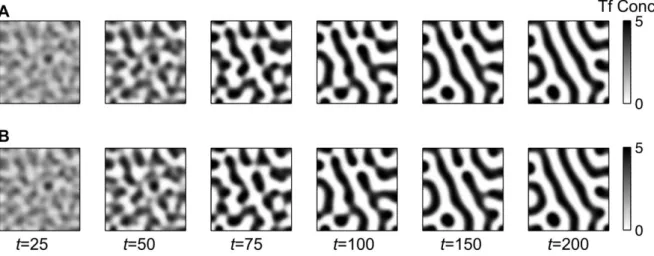
We illustrate this reduction in two situations. For the first, Activating situation, Fig. S4A represents the comparison of the pattern evolution at different time steps and with the same initial conditions. In the first row, the three-components model from the Main Text is used, while in the second row, the corresponding model reduction is illustrated. We observe that the pattern stabilizes with time in both cases in a similar manner (Fig. S4A vs. S4B).
In the third, Mixed I situation, however, we notice a particular phenomenon that highlights very well the transient nature of piebald patterns. In this situation, recall that 𝑓(𝑠) = 𝑠 and 𝑔(𝑠) = 1/𝑠. Assuming that 𝑆 has reached a quasi steady state makes the process faster. As such piebald patterns tend to disappear rapidly with time as illustrated in Fig. S5B vs. Fig. S5A. We may recover the results obtained with the two-components reduction when taking the initial condition 𝑆(0, 𝑥) at steady state in the three-components model (Fig. S5C).
To conclude and in the perspective of the application, a two-components reduction works well in generating classical Turing patterns, but may fail to represent precisely piebald phenomena, because of its sensitivity to initial conditions. Again, the main effect of this reduction is the loss of the factor 𝑟𝑣(𝑡). With the parameter 𝑟𝑣, seen as a scaling of the activation levels of the TF,
we can regulate the speed of the pattern formation. Moreover, such a reduction, with some parameters assumed to be large would also change the manner of estimating potentially important parameters and consequently the manner of understanding the biological phenomenon itself.
Regular patterns (Activating and Inhibiting situations) end up in a quasi-stationary, non-changing pattern at the infinite time point. The L2 norm of the discrete time-derivative, which is defined for the 𝑆 quantity tends to zero in these cases. This denotes
lim
𝑇𝑛→𝑇∞
||𝑆𝑇𝑛− 𝑆𝑇𝑛−1|| = 0
Figure S1. Linear stability analysis in the Activating and Inhibiting situations. (A) In the activating situation, the domain leading to the formation of Turing patterns is represented in blue as a function of the parameters 𝐷𝑎 and 𝑏𝑎; all other parameters are as in Fig. 2A-C, of the Main Text with 𝜎𝑎=
𝜎𝑖 = 0. (B-C) The same framework as in (A), but in an inhibiting case; see parameters of Fig. 2E-G of
the Main Text with 𝑏𝑖 = 1 and 𝐷𝑖 = 0.005 fixed in (B) and 𝑏𝑎= 0.9 and 𝐷𝑎= 0.005 fixed in (C) for a
similar framework as in Fig. 2E-G from the Main Text.
Figure S2. Bi-stability in the Mixed I situation and random initial conditions lead to piebald patterns. (A) Bifurcation diagram for the model leading to piebald patterns. The value of 𝐴𝑠 is computed
numerically and highlighted in blue, if linearly stable and in red, if instable as a function of the production rate 𝑏𝑖; all other parameters are as in Fig. 2H-J from the Main Text. For a certain range of
𝑏𝑖 values two linearly stable steady states coexist. (B) The basin of attraction of the steady state
𝐴𝑠 = 0.1, 𝐼𝑠= 124, 𝑆𝑠 = 0.01 as a function of the initial conditions on 𝐴, 𝐼, and 𝑆. Results were
Figure S3. Monostability in the Mixed II situation leads to color tones. A bifurcation diagram shows here that one unique (linearly stable) steady state is found within this framework. Parameters are as in Fig. 2L-M with 𝜎𝑎= 𝜎𝑖 = 0. This result was obtained by using Wolfram Mathematica 10.
Figure S4. Two-components and three-components models show a similar behavior in the Activating
situation. The parameters are set as in Fig. 2B of the Main Text, except that 𝑏𝑠= 20, 𝑑𝑠= 2, and
𝜎𝑎= 𝜎𝑖 = 0. (A) Representation of 𝑆(𝑡, 𝑥) simulated with the three-component model as reported
in the Main Text at different times 𝑡 until stabilization is attained and with 𝑆(0, 𝑥) ≡ 1. (B) Representation of 𝑆𝑠(𝑡, 𝑥) simulated with the reduced two-component model at the same time
Figure S5. The two-components and three-components model show quasi-similar behaviors in the
Mixed I situation with appropriate initial conditions. The parameters are set as in Fig. 2I of the Main
Text, except that 𝑏𝑠= 20, 𝑑𝑠= 2, 𝐷𝑎= 0.00005, 𝐷𝑖= 0.0000008, and 𝜎𝑎= 𝜎𝑖 = 0. (A)
Representation of 𝑆(𝑡, 𝑥) simulated with the three-components model as reported in the Main Text at different times points 𝑡 until stabilization and with 𝑆(0, 𝑥) ≡ 1. (B) Representation of 𝑆𝑠(𝑡, 𝑥)
simulated with the reduced two-components model at the same time points. The initial conditions for 𝐴 and 𝐼 are identical to the ones used in (A). (C) The same framework as in (A) but with initial conditions 𝑆(0, 𝑥) = 𝑆𝑠(0, 𝑥) for all 𝑥 in the domain.
Figure S6. Pattern stability in time. L2 norm of the time difference in values of S quantity tends towards zero both in the Activating and in Inhibiting situations.