HAL Id: hal-02333260
https://hal.archives-ouvertes.fr/hal-02333260
Submitted on 25 Oct 2019
HAL is a multi-disciplinary open access
archive for the deposit and dissemination of
sci-entific research documents, whether they are
pub-lished or not. The documents may come from
teaching and research institutions in France or
abroad, or from public or private research centers.
L’archive ouverte pluridisciplinaire HAL, est
destinée au dépôt et à la diffusion de documents
scientifiques de niveau recherche, publiés ou non,
émanant des établissements d’enseignement et de
recherche français ou étrangers, des laboratoires
publics ou privés.
Pairing GIS and distributed hydrological models using
Matlab 2
Sleimane Hariri, Sylvain Weill, Jens Gustedt, Isabelle Charpentier
To cite this version:
Sleimane Hariri, Sylvain Weill, Jens Gustedt, Isabelle Charpentier. Pairing GIS and distributed
hydrological models using Matlab 2. CAJG - 2nd Conference of the Arabian Journal of Geosiences,
Nov 2019, Sousse, Tunisia. �hal-02333260�
Pairing GIS and distributed hydrological models using
1
Matlab
2
Sleimane Hariri1, Sylvain Weill2, Jens Gustedt1,3, Isabelle Charpentier1 3
1
ICube UMR 7357, Université de Strasbourg&CNRS, 67412 Illkirch, France
4
2
LHyGeS UMR 7517, Université de Strasbourg&CNRS, 67000 Strasbourg, France
5 3 INRIA, France 6 [email protected] 7
Abstract. Observed data are required to carry out hydrological simulations
8
in a watershed for use by policy makers. Hydrological simulations thus require
9
a large interdisciplinary knowledge about modeling, computer sciences,
data-10
bases, GIS. A Matlab preprocess prior to the hydrological modeling is presented
11
for educational purposes and an easy uptake by non-GIS users. Moreover, this
12
allows for parallel computing. This pre-process builds on two renowned and
13
freely available Matlab toolboxes providing GIS and mesh functionalities.
Ad-14
ditional functionalities allow for a decomposition of watersheds with respect to
15
parameterized constraints, including the meshing of the subdomains and the
16
construction of an oriented flow graph. The method is exemplified on a
sub-17
basin of the Saar River.
18
Keywords: Hydrology, Domain decomposition method, GIS modelling.
19
1
Introduction
20
Data – topography, climate, land cover, soil properties – are required to carry out 21
hydrological simulations in a watershed for use by policy makers. These data are of 22
different nature and usually provided with their own standard data format. Topogra-23
phy and land cover are freely available from national agencies or transnational pro-24
jects like Copernicus or CORINE Land Cover. Climate data are scarcer in both time 25
and resolution. Fortunately, simulations can be performed using reanalyzes [1]. Soil 26
and geology parameters are usually unknowns and calibrated using climate data, dis-27
charge data and hydrological models. 28
Digital Elevation Models (DEM) store projected topographic information in a 29
gridded format and constitute fundamental data to hydrological studies [2]. Spatial 30
heterogeneities can be accounted by mean of a decomposition of the watershed into 31
smaller geographical units. Conceptual models preferably deal with sub-watersheds to 32
facilitate routing. River analyses are carried out using a one- or two-dimensional par-33
tial differential model discretized by meshing the major bed and splitting it longitudi-34
2
nally. Watershed simulations, surface and underground flows, involve more complex 35
meshes and numerical methods. Domain decomposition has another major advantage 36
since it offers the opportunity to run simulations on a parallel platform. 37
Only basic interdisciplinary knowledge in GIS, hydrology or computer sciences is 38
usually insufficient to carry out numerical simulations because pairing GIS tools, 39
database and computer models is not an easy task. QGIS and GMSH are loosely inter-40
faced by means of Python and shapefiles read/write. The Python-based open-source 41
framework PIHMgis [3] goes one step further by managing the coupling of GIS tools, 42
data and distributed hydrological modeling through pre- and post-processes. Although 43
a user interface exists and the program code is available, further developments require 44
a good knowledge of GIS tools, Python, and the programming language of the hydro-45
logical model under study. 46
To overcome this shortfall, Matlab is chosen as a framework for pairing GIS and 47
parallel/distributed hydrological models. Thereby, it enable to take advantage of exist-48
ing toolboxes [4,5]. This short paper presents a pre-processor written in Matlab that 49
allows for the management of DEMs with regards to hydrological structures, hydro-50
logical modeling and parallel computing. 51
2
Methods
52
The approach is to propose a user-friendly upgradeable open-source interface imple-53
mented in a classical language in sciences and educational communities. Matlab 54
meets these requirements and, additionally, it provides visualization functionalities. A 55
number of free toolboxes, namely TopoToolbox [4] and mSim[5], offer particular GIS 56
operations and mesh generation (through GMSH), respectively. Working in a non-57
GIS scientific computing framework rather than in a GIS or Python environment may 58
facilitate the uptake by engineering students. 59
The pre-process workflow ranges from the DEM read to watershed decomposition 60
and sub-mesh generation, carried out with respect to user’s constraints. 61
62
2.1 Domain decomposition 63
The watershed decomposition can be organized such that it fulfills parameterized 64
user-defined constraints: 65
1. the account for important hydrological structures (dams/ponds/discharge station) 66
or bridges that can create logjams. are “primary checkpoints”; 67
2. the partition of the domain into more sub-watersheds by placing “secondary 68
checkpoints” on the stream; 69
3. the design of sub-watersheds with similar areas, typically a few km². The inter-70
est is threefold: (i) assigning homogeneous data (soil and climate) at the sub-71
watershed level to account for spatio-temporal variability, (ii) dealing with hydro-72
logical sub-models of similar size, (iii) balancing the computational load on a par-73
allel platform. 74
All these checkpoints are inlets or outlets of the sub-watershed they delineate. At 75
surface level, these flow interfaces are located on the stream. Domain decomposition 76
functionalities are implemented by building on [4, 5] and Matlab. 77
78
2.2 Preprocess workflow 79
A graphical user interface (not shown here) articulates GIS and meshing operations as 80
follows: (1) read the DEM [4], (2a) define user outlets as suggested by the first con-81
straint, (2b) automatically insert additional outlets to satisfy the third constraint, (3) 82
partition the watershed by delineating drainage basins with respect to these outlets [4], 83
(4) format the partition as a shapefile for plotting purposes (shapewrite and shaperead 84
of the “mapping Matlab toolbox”), (5) mesh the subdomains [5], (6) determine inlet 85
and outlet faces, (7) order subdomains to build an upstream to downstream graph. 86
The files generated (sub-domain mesh and oriented flow graph) are used as input file 87
for the hydrological model. 88
3
Results
89
For the sake of clarity in the figures, the small watershed (89 km²) of the Mutterbach 90
stream near to the city of Sarralbe (Région Grand-Est, France) is used. To serve as a 91
defense waterline in 1940, 6 ponds and 5 dams were built to supply water and to con-92
trol the floods in the valley. These constitute a set of 11 primary checkpoints allowing 93
for water management. In Figure 1.b, the decomposition is carried out with respect to 94
these hydrological structures (marked with red squares). To anticipate parallel compu-95
ting, secondary checkpoints have been added to fulfill the third constraint. Figure 1.c 96
displays a decomposition into 58 subdomains, the areas of which range from 1 km² to 97
2.5 km² with an average value of 1.54 km². The numbers of nodes/elements in the 98
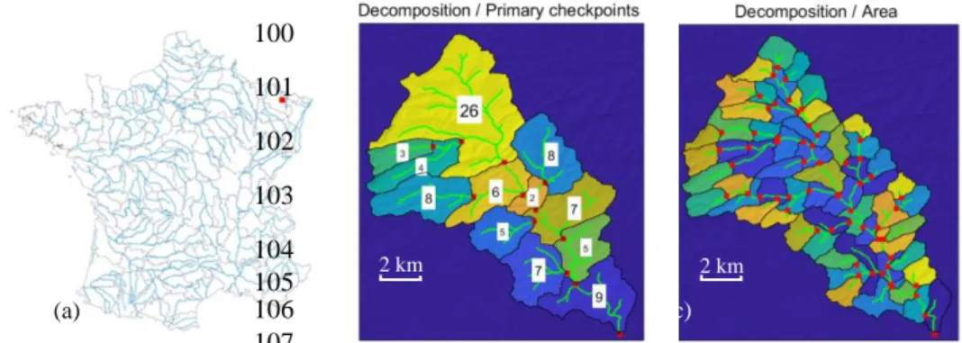
sub-meshes are equal to 1260/2200 on average, respectively. 99 100 101 102 103 104 105 (c) 106 107
Fig. 1. (a): Location in France (red point); (b): Decomposition/checkpoints; (b)
Load-108
balanced refined decomposition.
109
2 km 2 km (a)
4
4
Discussion
110
Hydrological simulations require a large interdisciplinary knowledge about modeling, 111
computer sciences, databases, GIS… For educational purposes and an easy uptake by 112
non-GIS users, our interdisciplinary team (hydrologists, computer scientists and 113
mathematicians) work on Matlab pre- and post-processes to the hydrological model-114
ing. These build on two renowned and freely available Matlab toolboxes [4,5] provid-115
ing GIS and mesh functionalities, respectively. Note that both were designed in a 116
hydrological context and come with user guides. 117
For the sake of reproducibility, proposed domain decomposition functionalities 118
(parameterized constraints, watershed decomposition and oriented flow graph) will be 119
exhaustively described and documented in a future work. Then, Matlab codes will be 120
made freely available to serve as a basis to implement other decomposition con-121
straints. Complementary tests were performed on the Saar watershed partly located in 122
France and Germany. 123
This hydrology-targeted Matlab-GIS framework is intended to be useful not only 124
for education purposes or for a first contact with GIS tools for hydrology modeling, 125
but also as a common basis for interdisciplinary studies with non GIS users. Moreo-126
ver, it benefits from the numerous toolboxes already developed in and for Matlab. 127
5
Conclusion
128
The Matlab-GIS interface builds on two renowned and freely available Matlab 129
toolboxes providing GIS and mesh functionalities. It has been designed for an easy 130
uptake by non-GIS users and modelers in hydrology. Resulting watershed decomposi-131
tion can be interfaced with a conceptual model or with a parallelized finite element 132
model for watershed simulations by using the oriented flow graph for routing. 133
References
134
1. Caillouet, L., Vidal, J.-P., Sauquet, E., Graff, B., Soubeyroux, J.-M: SCOPE Climate: a
135
142-year daily high-resolution ensemble meteorological. reconstruction dataset over
136
France. Earth System Science Data 11(1), 241–260 (2019).
137
2. McDonnell, R.A.: Including the spatial dimension: Using Geographical Information
Sys-138
tems in hydrology. Progress in Physical 20(2), 159–177 (1996).
139
3. Bhatt, G., Kumar, M., Duffy, C.J.: A tightly coupled GIS and distributed hydrologic
mod-140
eling framework. Environmental Modelling & Software 62(), 70–84(2014).
141
4. Schwanghart, W., Kuhn, N.J.: TopoToolbox: A set of Matlab functions for topographic
142
analysis. Environmental Modelling & Software 25(6), 770–781(2010).
143
5. Kourakos, G., Harter, T.: Vectorized simulation of groundwater flow and streamline
144
transport. Environmental Modelling & Software 52, 207–221 (2014).