Education and health care in developing countries

Education and Health Care in Developing Countries

by

Trang V. Nguyen

B.A. Economics and Mathematics

Brandeis University, 2003

Submitted to the Department of Economics

in partial fulfillment of the requirements for the degree of

Doctor of Philosophy

at the

MASSACHUSETTS INSTITUTE OF TECHNOLOGY

September 2008

©2008 Trang V. Nguyen. All rights reserved.

The author hereby grants to MIT permission to reproduce and to distribute publicly paper

and electronic copies of this thesis document in whole or in part in any medium now

known or hereafter created.

Signature of Author...

Department of Economics

August 1, 2008

Certified by...

...

Esther Duflo

Abdul Latif JamM, Professor of Poverty Alleviation and Development Economics

Thesis Supervisor

Certified by...

Abhijit Banerjee

Ford International Professor of Economics

Thesis Supervisor

Accepted by....

Peter Temin

Elisha Gray II Professor of Economics

Chairman, Departmental Committee on Graduate Studies

Education and Health Care in Developing Countries

by

Trang V. Nguyen

Submitted to the Department of Economics on August 15, 2008, in partial fulfillment of the

requirements for the degree of Doctor of Philosophy

Abstract

This thesis is a collection of three essays on education and health in developing countries.

Chapter 1 shows that increasing perceived returns to education strengthens incentives for schooling when agents underestimate the actual returns. I conducted a field experiment in Madagascar to study alternative ways to provide additional information about the returns to education. I randomly assigned schools to the role model intervention, the statistics intervention, or a combination of both. I find that providing statistics reduced the large gap between perceived returns and the statistics provided. As a result, it improved average test scores and student attendance. For those whose initial perceived returns were below the statistics, test scores improved by 0.37 standard deviations. Seeing a role model of poor background has a larger impact on poor children's test scores than seeing someone of rich background. The key implication of my results is that households lack information, but are able to process new information and change their decisions in a sophisticated manner.

Chapter 2, joint work with Gerard Lassibille, evaluates several interventions in Madagascar that sought to promote top-down and local monitoring of the school to improve education quality. Randomly selected school districts and subdistricts received operational tools to facilitate their supervision tasks. Randomly selected schools in these treated districts were reinforced with teacher tools and parent-teacher meetings centered around a school report card. We find little impact of targeting district and sub-district administrators. Meanwhile, the intervention implemented at the school level improved some of the teachers' behaviors and student attendance. Student test scores also improved by 0.1 standard deviations after two years. These results suggest that beneficiary monitoring is more effective than mediated control in the hands of

government bureaucrats in this context.

Chapter 3 studies informal payments to doctors and nurses for inpatient health care in Vietnam. Exploiting within-hospital variation, I find that acute patients, despite having a presumably higher benefit of treatment, are 8 percentage points less likely to pay bribes, and pay less, than non-acute patients. One plausible interpretation is that doctors might face existing incentives against neglecting acute cases. I find that the differential payment by acute status is larger in central locations (expected to be well-monitored) and at facilities that receive more audit visits. Overall, these findings may be a sign of bureaucrats responding to incentives, even in a highly corruptible environment.

Thesis Supervisor: Esther Duflo

Title: Abdul Latif Jameel Professor of Poverty Alleviation and Development Economics Thesis Supervisor: Abhijit Banerjee

Acknowledgments

I am very grateful to my advisors, Esther Duflo, Abhijit Banerjee, and Tavneet Suri. Their passion for development economics and continual support have inspired and guided me throughout my graduate studies, by much more than what can be expressed here.

This thesis has benefited from discussions with the faculty and students at MIT and other institutions. David Autor, Suman Basu, Jim Berry, Miriam Bruhn, Quoc-Anh Do, Quy-Toan Do, Rachel Glennerster, Michael Greenstone, Rick Hornbeck, Rob Jensen, Cinthya Kinnan, Ben Olken, Rob Townsend, and participants of the MIT development and applied micro lunches have provided very valuable suggestions. My research in Madagascar would not have been possible without the diligent and excellent work by the AGEMAD team at the Madagascar Ministry of Education, Jee-Peng Tan, Comelia Jesse, and Gerard Lassibille. I am grateful to Greg Fischer and Raymond Guiteras for their comments, everyday encouragements, and ready hands of help. I thank especially Maisy Wong for sharing her kind support, insights, and friendship.

I have been fortunate to receive generous financial support from the World Bank, AFD, UNICEF, and the TOTAL Fellowship for part of the research in this dissertation.

I would like to thank all my friends and family for their optimism and understanding during the past five years. Having Tatiana Didier, Chris Smith, and Tom Wilkening as classmates and housemates made graduate school an enjoyable experience. My partner Duc, my brother Quan, and my Murray family made me laugh and kept my life balanced during tough times.

I dedicate this dissertation to my parents, Nguyen Xuan Phuc and Nguyen Thi Thuy Van. Their love and belief in me make it a worthwhile path through every challenge and success.

Contents

1 Information, Role Models and Perceived Returns to Education:

Experimental Evidence from Madagascar 9

1.1 Introduction 9

1.2 A Model of Schooling with Uncertainty about the Return to Education 13

1.2.1 Model Setup 14

1.2.2 Updating Based on Statistics 16

1.2.3 Updating Based on Role Models 17

1.2.3.1 Individual's Problem 18

1.2.3.2 Government 19

1.2.3.3 Equilibrium Concept (Benchmark Model) 20

1.2.4 Statistics and Role Models 21

1.2.5 Discussion 22

1.3 Study Design 23

1.3.1 Description of the Intervention 23

1.3.2 Sample and Evaluation Design 26

1.4 Data and Experimental Validity 27

1.4.1 Data 27

1.4.1.1 Background Data 27

1.4.1.2 Perception of Returns to Education 28

1.4.1.3 Schooling Outcomes 30

1.4.2 Experimental Validity 30

1.5 Estimation Strategy and Results 32

1.5.1 Baseline Perceived Returns to Education 32

1.5.2 Estimation Strategy 33

1.5.3 Impact on Perceived Returns 35

1.5.3.1 Impact of Statistics on Perceived Returns 35 1.5.3.2 Impact of Role Models on Perceived Returns 37

1.5.4 Impact on Education Investment 38 1.5.4.1 Impact of Statistics on Education Investment 38 1.5.4.2 Impact of Role Models on Education Investment 40

1.5.5 External Validity 40

1.6 Conclusion 41

2 Improving Management in Education:

Evidence from a Randomized Experiment in Madagascar 59

2.1 Introduction 59

2.2 Primary Education System in Madagascar 63

2.3 The AGEMAD Interventions 65

2.3.1 Description and Structure of the Program 65

2.3.2 Why Might We Expect These Interventions to Work? 69

2.4 Evaluation 70

2.4.1 Data Collection 70

2.4.2 Descriptive Statistics 72

2.4.3 Attrition 72

2.5 Estimation Strategy and Results 73

2.5.1 Intermediate Outcomes at School 74

2.5.1.1 Impact of CISCO and ZAP Interventions on

Intermediate Outcomes 74

2.5.1.2 Impact of School Intervention on Intermediate Outcomes 76

2.5.2 Behaviors of ZAP and CISCO Heads 77

2.5.3 Student Attendance and Dropouts 79

2.5.4 Learning 81

2.6 Conclusion 81

3 Incentives against Corruption in Acute Health Care in Vietnam 100

3.1 Introduction 100

3.2 A Model of Side Payment and Illness Condition 104

3.3 Background and Data 107

3.3.2 Informal Payment ₁₀₈

3.3.3 Data 109

3.4 Estimation Strategy and Results 111

3.4.1 Acute Conditions ₁₁₃

3.4.2 High-Bribe Locations 114

3.4.3 Interpretation ₁₁₅

3.4.4 High-Incentive Locations 117

Chapter 1

Information, Role Models and Perceived Returns to

Education: Experimental Evidence from Madagascar

1.1

Introduction

Universal primary enrollment is one of the Millennium Development Goals, and many countries, especially those in Africa, have devoted substantial efforts to attaining this objective. Nonetheless, low schooling persists even though market returns to education appear to be high and direct costs are low.' For example, in Madagascar, the estimated returns to one extra year in primary and secondary school are 5% and 12%, respectively. Primary education is free; yet, 40% of children entering first grade actually complete five years of primary school. Only half of those children who complete primary school continue on to secondary school. Even when children are enrolled, low learning, as reflected in the 63% pass rate at the primary-cycle examination, is an important concern (Tan 2005). In addition to low achievements, widespread student absenteeism during the school year suggests low effort on students' part.

While there can be several explanations for low schooling such as credit constraints, high dis-count rates, or low school quality,2 I focus on another possibility: an information gap between perceived returns to schooling (what people consider to be the returns) and actual returns. Such a gap can exist due to costly gathering of information in isolated areas of developing countries. My paper documents this information gap in rural Madagascar. Households appear to have imperfect information about earnings associated with different levels of education, even in the presence of heterogenous returns. They will choose low education when they think the return is low (Foster and

'Psacharopoulos (1985) and Psacharopoulos (1994) estimate the returns to be high in many developing countries.

2

For example, Oreopoulos (2003) explores the possible role of high discount rates in the decision of high-school dropouts. See Glewwe and Kremer (2005) for a more complete review.

Rosenzweig (1996) and Bils and Klenow (2000)). Thus, we would expect that increasing perceived returns can strengthen incentives for schooling for those who may have initially underestimated the returns.

Once we know there is imperfect information about the returns to education, the next important step is to examine how to provide useful additional information. One straightforward way is to

provide statistics. The downside of this approach is that a largely illiterate population may not effectively process statistical numbers. An alternative way of informing households of the benefits of education is through a "role model," i.e. an actual person sharing his success story. This policy choice has been more popular than presenting numbers (for example, UNICEF has role model programs in various developing countries). Role models can be effective simply because stories are powerful, or because they contain information. Wilson (1987) proposes that role models bring back missing information about the upside distribution of returns to education. The impact of observing a role model will depend on how households update their beliefs based on the information the role model brings. Ray (2004) suggests that role models might be powerful only when they come from a similar background and, therefore, carry information relevant to the audience.3

My paper sheds further light on how to provide additional information about the returns to education. I ask the following three questions: (i) Are households' perceived returns to education different from the estimated average return, due to heterogeneity entirely or also imperfect infor-mation? (ii) How do households update beliefs when presented with statistics about the average return or with a specific role model? (iii) How do children adjust their efforts in response to the change in perceived returns? To address these questions, I first administered a survey in rural Madagascar to measure parents' perceived returns for their child and perceived returns for the average person in the population.4 I then conducted a field experiment in 640 primary schools, in

3

Discussions on role models have featured both in the policy environment and in the academic literature. Most of the evidence to date focuses on a "mentoring" role model; for example, a teacher of the same race has a positive impact on a student's test scores (Dee 2004). My work studies a role model's informational effect, i.e. how people update beliefs based on the information the role model brings.

4

conjunction with the Madagascar Ministry of Education. The experimental design was motivated by a model of schooling decisions with heterogeneous returns and uncertainty about the return to education. When an agent is presented with the statistics, he updates his belief about the average return. When presented with a role model, he infers that heterogeneity in the returns to education is high, making the statistical estimate of the average return less relevant. Thus, role models will undermine the impact of the statistics intervention. The agent also infers from the role model's background that individuals from this background receive relatively high returns to education on average.

To test the theory's key predictions, I randomly assigned schools into three main treatment groups. In the "statistics" schools, teachers reported to parents and children the average earnings at each level of education, as well as the implied gain. The second intervention sent a role model to share with students and families his/her family background, educational experience, and current achievements. To investigate the proposition that a role model from the same background carries relevant information, I randomly assigned a role model of poor or rich background to different schools. The third treatment combines both the statistics and role model interventions together, investigating the possibility that role models may undermine statistics. I collected endline data on perceived returns, student attendance, and test scores to evaluate the impact of the interventions on beliefs and on effort at school roughly five months later.

I find that parents' median perceived return matches the average return estimated from house-hold survey data. Nonetheless, there is a lot of dispersion in both perception of the average return and perception of the child's own return. There are two possible explanations for dispersion in perception of the child's own return: heterogeneity in the actual returns and imperfect informa-tion. I argue that while heterogeneity plays a role, some extent of imperfect information exists, as

(1992) first brought this topic to attention by proposing that youths infer the returns from their sample of observations. Several papers have surveyed college students in the US for their perceptions of incomes associated with different educational levels: Betts (1996), Dominitz and Manski (1996), Avery and Kane (2004). Most find that American students estimate quite well the mean earnings for a cohort, and think they would earn slightly better than the mean.

reflected in the larger dispersion in perception than in the real distribution of earnings.

The main results of the experiment match the model's predictions. Participants who received the statistics intervention updated their perceived returns. Providing statistics significantly de-creases the gap between perceived returns and the estimated average return provided. This result holds for both perception of the average return and perception of one's own return. It suggests that part of the dispersion in perceived returns comes from imperfect information. Once house-holds update their perceived returns, schooling decisions consequently respond. The statistics intervention improved average test scores by 0.2 standard deviations, only a few months later. For those whose initial perceived returns were below the statistics, test scores improved by 0.37 stan-dard deviations. Student attendance in statistics schools is also 3.5 percentage points higher than attendance in schools without statistics.

The role model interventions offer very interesting results. By themselves, role models have small effects on average, but people seem to care about the information the role model brings. In particular, consistent with the theory, the role model's background matters. The role model from a poor background improved average test scores by 0.17 standard deviations, while the role model from a rich background had no impact. Moreover, this positive impact of poor-background role models on average test scores mainly reflects their influence on the poor (0.27 standard deviations). Again as the theory predicts, combining a role model with statistics undoes the effects of statistics. The role model may indicate high underlying heterogeneity in individual returns, implying that the statistics were imprecisely estimated. Thus, households do not update as much based on the statistics as they would otherwise.

These results have strong implications. First, households update their perception in a sophis-ticated way based on the information provided. Second, schooling investment seems responsive to changes in perceived returns. Third, in terms of policies to improve education in developing countries, providing statistical information can be a cost-effective instrument to enhance children's efforts at school, in contexts where individuals underestimate the returns. A quick

back-of-the-envelope calculation using my results shows that the statistics intervention would cost 2.30 USD for an additional year of schooling and 0.04 USD for additional 0.10 standard deviations in test scores (cheaper than any prior programs evaluated with a randomized design). Lastly, when households do have correct perception of the returns on average, the results from this paper suggest that mar-ket interventions to improve the overall returns are an important way to increase school attendance and test scores.

Some existing evidence already shows that the provision of information may affect individual behaviors, such as Dupas (2006). In particular, Jensen (2007) demonstrates from a field experiment in the Dominican Republic that providing students with mean earnings by education led to a 4 percentage point increase in the probability of returning to school the following year. My work builds on this result along two fronts. First, I test whether statistics given to the parents affects the intensive margin of schooling-student attendance and test scores. Second, in terms of the research question, I study whether role models are effective in changing behaviors, either through their success story or through the relevance of their information. Addressing this research question would provide more depth to our understanding of how people update their belief.

The rest of this paper is organized as follows. Section 1.2 discusses a model of schooling decisions under Bayesian updating of perceived returns. In Section 1.3, I describe the field experiment: the statistics and role model programs, as well as the evaluation design. Section 1.4 discusses the data. Section 1.5 gives an overview of perceived returns to education at baseline, and then presents the estimation strategy and results. The final section concludes.

1.2

A Model of Schooling with Uncertainty about the Return to

Education

To assess the conditions under which the statistics and role model programs may plausibly affect decisions, this paper integrates a simple framework of schooling with Bayesian updating about

the return to education. This theory builds on the standard Card (1999) model of school choice with heterogeneity in individual returns to education. Here I formalize the possibility that agents measure their own return as well as the average return with errors. As a result, I explore two features of learning.

First, this section models learning about the average return to education. I show that agents update their estimate after observing the government's statistic on the average return. How much they update depends on their belief about the precision of the government's estimate. When there is high heterogeneity in individual returns in the population, the government's estimate of the average return is less precise. In that case, agents should put less weight on this statistic.

Second, an agent also learns about the relationship between his type and his return to education, above and beyond the population's average return. He infers this information from observing the government's choice of role model programs. School investment decisions are then made based on the posterior belief about the return to education.

1.2.1

Model Setup

Consider individual schooling choice under heterogeneous returns to education. An individual i has the following preferences5

EU = Ei In yi(ei) - ci(ei) (1.1)

where log earnings is a linear function of education Inyi(ei) = ai + biei and ci(ei) denotes an increasing and convex cost function of education. In the standard model of investment in human capital, ei represents years of schooling. Here I examine effort behaviors of children already enrolled in school. I refer to ei as child effort in schooling, but the general intuition from the standard

5I abstract from risk aversion here. Modeling log earnings as concave in the return to education bi does not change the nature of updating perception.

model remains. The optimal choice of effort solves the first-order condition

Ei[bi] = c:(ei) (1.2)

Given that marginal cost is increasing in ei, the optimal choice of effort will increase if the individual expects higher returns.

The individual's true return to education is determined by the actual average return in the population and by some heterogeneity factors (observable and unobservable characteristics)

bi = b + Xi/ + Ei (1.3)

where b denotes the actual average return in the population; for example, when the whole economy is doing better, everyone has higher returns. Xi is some observable characteristic that affects one's own return, such as parental wealth (rich or poor background). The last term ei captures any heterogeneity unobserved to others and only known by the individual, such as ability. Let ei be normally distributed ei - N(O, a ).

Uncertainty about one's own return comes from two sources: imperfect knowledge of the av-erage return (b) and that of the relationship between his characteristics and his own return (y). First, assume as in the Bayesian approach that the individual's belief can be described as a prior distribution on the actual average return b - N(bo, C ). His perceived average return is Ei[b] =- bo =

b + ±i. Second, he does not perfectly observe y either: Ei[7] =

y

Ei [b]

=

Ei [b]

+ Ei[Xi7] +

ei

(1.4)

Perceived Self Perceived Average

=

(b + Xiy + E) + (i + Xi?)

(1.5)

With this framework in mind, the next subsection models how individuals update their perceived return after the statistics and role model interventions.

1.2.2

Updating Based on Statistics

Suppose the government receives a noisy signal about the average return bc = b + (G. The government's noise is normally distributed (G - N(0, o-2), i.e. the precision of its signal is 1/.g The government provides this statistic be to all agents. As the individual sees the government statistic about the average return, he will update his estimate of the average return toward that number. Bayesian updating leads to a normal posterior distribution (DeGroot 1970), with the following mean and variance

aE b bo=+ 2 b (1.6) 2 2

E[baIbG]

(1.7)

Vari[blbG]=

2 G2

(1.

The individual's posterior perceived average return is a weighted average of his prior and the government statistic. The weight depends on the precision of the government's signal: if U2 is small, the posterior becomes very close to the statistic. To elaborate, suppose the government's signal bG comes from random sampling of n observations in the population. The variance of its estimate is 2G = -, where s2 is an estimate of the population variance. That is, the government's signal is less precise when there is high underlying heterogeneity in the population. I will return to this point later when I discuss heterogeneity in more detail.

According to expression 1.4, agents will also update their own expected return toward the statistic. For people who had initially underestimated the average return (bo < bc), their perceived

return increases, resulting in higher effort e. However, one's relative position to the average Ei [XX<] + ei is still unchanged.

1.2.3

Updating Based on Role Models

The next step is to examine how individuals update their belief after seeing a role model. The role model is simply one observation from the distribution and should not affect beliefs unless this person carries a signal about the return to education. I need to model explicitly what an individual thinks the role model is supposed to signal and why the government chooses to send information in this way. A useful framework in which role models might plausibly affect behaviors is a game between the government and an individual. I formalize individuals' beliefs about the programs and their behaviors in a Perfect Bayesian equilibrium. Recall that each agent is uncertain about the relationship between his characteristics and his own return (-y). Here a welfare-maximizing government receives a signal about this relationship. Through its role model programs, it conveys the information to people.

First, let me specify the observable characteristic Xi to be the individual's type. Suppose there is a continuum of agents of measure 1. There are 2 types H and L (born rich and poor). One's type is unknown to other individuals but observable to the government. Perceived return in expression 1.4 can now be written as

Ei[bi] = Ei[b] + E(QH) * H + E( yL) * L + Ei (1.8)

where H and L are dummies for each corresponding type. Without loss of generality, I look at an L-type individual throughout the rest of the model. He does not observe 'YL perfectly.

There are 3 states of nature with varying individual return. The "low heterogeneity" state occurs with probability 1 - q, in which case returns to education do not depend on one's type, i.e. YH =- L = 0. I call this state "low heterogeneity" since heterogeneity in individual returns in the population comes solely from unobservable (a,) rather than from both observable and unob-servable characteristics. Alternatively, when there is high heterogeneity (with probability q), this heterogeneity favors one type. In the good state ("good" from the L-type's point of view), being of

type L affects the return positively 'YL = 72 > 0 while being of type H affects the return negatively

'H '71 < 0. Symmetrically, in the bad state, 7L = 71 < 0 and TH = 72 > 0. There is uncertainty about the state. The probability of high heterogeneity is q , and the probability of the good state given high heterogeneity o0.

Definition 1 After the payoff is realized, anyone with income above a threshold y is considered to be successful ("role model").

Consider a static game between 2 players: a welfare-maximizing government and a low-type individual. The timing is as follows. Nature first decides on low or high heterogeneity. Under high heterogeneity, nature decides which type has the higher return (good or bad state for the L-type). The government knows exactly which state it is. The government decides whether to send a role model-example of success, and which type to send. The individual sees the government's action and infers information about the state. He then updates beliefs about the return using Bayes' rule, and chooses the optimal level of effort. The extensive form of the game is displayed in Appendix Figure 1.

1.2.3.1 Individual's Problem

Given the prior beliefs, a low-type individual's expected rate of return is

Ei[bi] = Ei [b] + 4q0

7

q(1

+

His choice of e solves

eo = arg max{[Ei[b] + qfoz0 2 + q(1 - Po)71 + ei]e - ci(e)} (1.10)

In the low heterogeneity state:

elowhet = arg max{ [Ei [b] + ei]e - ci(e)} (1.11)

In the good state:

egood = arg max{[E [b] + + ei]e - ci(e)} (1.12)

In the bad state:

ead = arg max{[Ei [b] + -y + ei]e - ci (e)} (1.13)

1.2.3.2 Government

The welfare-maximizing government receives a fully informative signal of what the state is. It wants to choose an action to signal to the low-type agent about the state so that he can make the efficient choice of effort. The government wants the individual's choice to be as close as possible to the efficient choice. Consider the government's set of possible strategies g E {Nobody, L, H}, which represents sending nobody, sending a low-type role model, or sending a high-type role model.

Given a signal status s E {Lowhet, Good, Bad}, the government's objective function is

minle(g) - e*(s)I (1.14)

g(s)

where e(g) is the response function of the low-type after observing the government's action g. e*(s) is the efficient effort level under each of the government's information sets

e*(Lowhet) = eh• = argmax{[Ei[b] + ei]e

-

ci(e)}

(1.15)

e*(Good) - e*ood = argmax{[Ei[b] + 72 + ei]e - ci(e)} (1.16)

e*(Bad) -

ead = argmax{[Ei[b] +1 + ei]]e - ci(e)}

(1.17)

1.2.3.3 Equilibrium Concept (Benchmark Model)

Proposition 2 The following strategies and beliefs constitute a (pure-strategy) Perfect Bayesian equilibrium.

Government's strategy g(s): g(Lowhet) = Nobody, g(Good) = L, g(Bad) = H Low-type individual's strategy e(g): e(Nobody) = elowhet, _{e(L) = egood, e(H) = ead} Individual beliefs at his decision node:

probability[Lowhetlg = Nobody] = 1

probability[Goodlg = L] = 1 probability[Badlg = H] = 1

Proof. We need to show that each strategy is the best response given the other party's strategy, and the beliefs are consistent with Bayes' rule.

At the final decision node, the low-type individual updates his belief on the state after observing the government's move. Given the government's strategy, seeing g = Nobody means that the government signals the low heterogeneity state. Given the government's equilibrium strategy, the individual's posterior belief is probability[Lowhetlg = Nobody] = 1. The solution to his maximization problem is elowhet (see expression 1.11). Seeing g = L implies that the state is good, so the individual updates

prob[goodlg = L] (1.18)

p[LIgood] * q _(1.19)

p[Llgood]qpo + p[LJbad]q(1 - po) + p[Lllowhet](1 - q)

S1 * qpo _(1.20)

1 * ql-o + 0 * q(1 - po) + 0, (1 - q)

= 1 (1.21)

This is good news (also better news than seeing nobody) since he now thinks his return is Ei[b] +

model is bad news to the low-type individual, and leads to ead.

Given the individual's strategy, the government solves its minimization problem as in expression 1.14. It would not deviate from the equilibrium strategy since that would cause the individual to deviate from the efficient choice of effort. n

1.2.4

Statistics and Role Models

This subsection summarizes the predictions of updating based on statistics and on role models from the previous two subsections, taking into consideration the effect of the combined interventions. Now in equilibrium, sending role models implies high underlying heterogeneity in the population. Recall that the government's statistic bc is less precise under high heterogeneity. As a consequence, the individual puts less weight on the government's statistic when the government also sends a role model.

The equilibrium strategies in the previous benchmark model can be extended to the following. Government's strategy:

1. No signal about the average return, low heterogeneity state: do nothing

2. Noisy signal about the average return, low heterogeneity state: provide statistics alone

3. No signal about the average return, high heterogeneity state: send low-type role model if good state, send high-type role model if bad state

4. Noisy signal about the average return, high heterogeneity state: provide statistics, and a role model as in strategy 3.

Low-type individual's strategy:

1. Government does nothing: infer that it is the low heterogeneity state and choose effort ac-cordingly

2. Statistics alone: update perceived returns Ei[b] and Ei [bi], infer that it is the low heterogeneity state, and change effort

3. Low-type role model: infer that it is the good state and increase effort

4. High-type role model: infer that it is the bad state and decrease effort

5. Statistics and low-type role model: update perceived returns, infer that it is the good state but put less weight on the statistics, and change effort

6. Statistics and high-type role model: update perceived returns, infer that it is the bad state and put less weight on the statistics, and change effort

These strategies give us a set of predictions for individual behaviors under the government's statistics and role model programs explored empirically in this paper.

1.2.5

Discussion

There are three important numbers here that will be relevant throughout the rest of the paper. The government has a signal bc about the actual average return b, and this is the statistic it provides. People initially do not know b and have a perceived return for the average Ei[b] - bo = b + (j. Each individual also has expected return for his own type, i.e. a perceived return to education for himself as in expression 1.4.

When mapped to the empirical setting, this model carries three main insights. First, it predicts that everyone updates toward the statistic about the average return. In particular, this statistic has the same effect for two individuals of different types who start with the same prior about the average return. Second, seeing a role model of the same type (initial background) is good news since this role model reveals to the agent that the heterogeneity is favorable to him. Meanwhile, seeing a role model from a different type is bad news. Third, combining statistics with a role model may signal high heterogeneity in the returns and undermine the impact of statistics.

The sections that follow will explore how people behave empirically when they receive the statistics and role model programs from the government.

1.3

Study Design

Imperfect knowledge of the return, as described in section 1.2's framework, is arguably common in many areas in developing countries. Most of rural Madagascar lies in secluded areas with limited access to outside information, and information on earnings is not covered by the media (radio). According to a pilot study by the Ministry of Education and UNICEF in November 2006, many local parents have difficulties estimating the income associated with various educational attainments. From my survey data, 73% of the respondents report that it is difficult to learn about their peers and neighbors' income; 53% say there are frequent incidences of educated people out-migrating from the village. These observations suggest that rural households might have considerable uncertainty about the returns to education.

1.3.1 Description of the Intervention

To learn about behavioral responses to role models and to returns to education statistics, I designed a field experiment to be carried out by the Ministry of Education (MENRS), with support from the French Development Agency (AFD), UNICEF, and the World Bank. This experiment was implemented as a government program, and households presumably responded in this context. The government programs evaluated here were launched at mid-school year, in February 2007 (the academic calendar in Madagascar runs from September to June).

One important feature of the design was that all participating schools organized a parent-teacher meeting. In the comparison group, parents and parent-teachers discussed during this meeting any typical topics of the school.6

In the other program schools, in addition to these discussions,

6

This placebo treatment allows me to avoid confounding the effects of meetings mandated by the government with the effects of statistics or role models. For example, I control for the potential impact coming from teachers

Grade 4 students and their parents received either the "statistics" intervention, the "role model" intervention, or both during this meeting.

First, the "statistics" intervention sought to inform parents of the average returns to education, calculated from the nationwide population. In this treatment, school teachers first presented a few simple statistics based on the 2005 Madagascar Household Survey (Enquite aupres des M6nages) to all Grade 4 students and their parents at a school meeting. For each education level, the audience learned about the distribution of jobs by education, and the mean earnings of 25 year-old Malagasy females and males by levels of education. Then the teacher explained the magnitude of increased income associated with higher educational levels, therefore implying percentage gains or returns to education. Discussion on these statistics lasted about 20 minutes. Parents also received a half-page information card featuring mean earnings by gender and by education, and a visual demonstration of the percentage gain (see sample card in the Appendix Figure 2). I refer to these statistics as the estimated average returns to education (bG in the model). The numbers reported to families are predicted values from a Mincerian regression of log wage on education levels, age, age squared, and gender. These estimates are robust to adding region of birth fixed effects, but they may be biased due to potential endogeneity problems. Within the experiment, people should still respond to the new information provided that these estimates differ from their prior perception.

Second, the role model program mobilized three types of local role models to share their life story at treated schools. In this context, a "role model" is an educated individual with high income,

who grew up in the local school district.7 Motivated by the theoretical proposition that role models from different backgrounds carry different information, I randomly assigned a role model of poor or rich background to different schools. In practice, it was important to also have a role model of moderate income, possibly the relevant level of success for certain areas. The exact types are

suddenly becoming concerned that the government is paying attention to them, or any motivation to parents from being involved in the school.

7_{Existing definitions of role models vary. A broader definition of a role model refers to any example of success that}

defined as follows:

* Role Model type LM (low to medium): a role model of low-income background similar to many students in the audience (the father and mother were farmers, the role model went to the village school, for example) who is now moderately successful (generating high productivity on farm, or owning a profitable shop)

* Role Model type LH (low to high): a role model of low-income background similar to many students in the audience, who is now very successful (government official or manager of a big enterprise, earning high income).

* Role Model type HH (high to high): a role model of high-income background (father works for government, mother is a school teacher, the role model went to a private preparatory school, for example) who is now very successful.

Through a local committee consisting of the school district head, a local NGO leader, and community leaders, MENRS identified and recruited 72 role models of different types between December 2006 and January 2007. This recruitment made no explicit distinction in terms of gender (and it turned out there were 15 female role models). UNICEF Communication Sector provided two days of training on communication skills to the chosen role models so that they could reflect on their personal experiences, write an abbreviated script and practice an oral presentation. This training only guided the stories to cover at least three bases of information: background, educational experiences, and current job and standard of living. These role models then visited selected schools (one visit per school) and shared their life stories with all 4th-graders and their parents at a school meeting. After the role model's speech (about 20 minutes), the meeting proceeded to questions and answers, and open discussions. According to field reports, the topics of discussions were mostly to clarify the role model's story, but the parents also expressed their doubts. They sometimes cited examples of teenagers in their village with a high school degree but without a permanent job.

Most frequently, they justified the difficulties of sending children to schools during periods of food shortages.

Finally, in the combined treatment schools, both of the above interventions took place at the same school meeting. The school teacher first explained returns to education statistics, followed by the role model's exposition.8 The school meetings were well-attended throughout my study sample.

1.3.2 Sample and Evaluation Design

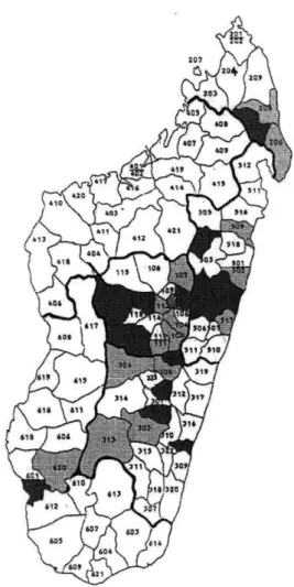
The study sample consists of 640 public primary schools in 16 districts throughout rural Madagascar (see the map in Figure 1). To arrive at this study sample, I had excluded from the Ministry's roster a few schools that are too far away and extremely difficult to access. These 640 schools were divided into 8 groups of 80 each, to receive different combinations of the aforementioned "statistics" intervention, role model interventions and their combinations. Treatment assignment into the 8 groups was random, stratified by students' baseline test score and AGEMAD treatment status. AGEMAD is an on-going experiment aimed at improving management in the educational system, which also covered all the schools in my sample (Nguyen and Lassibille 2007).9

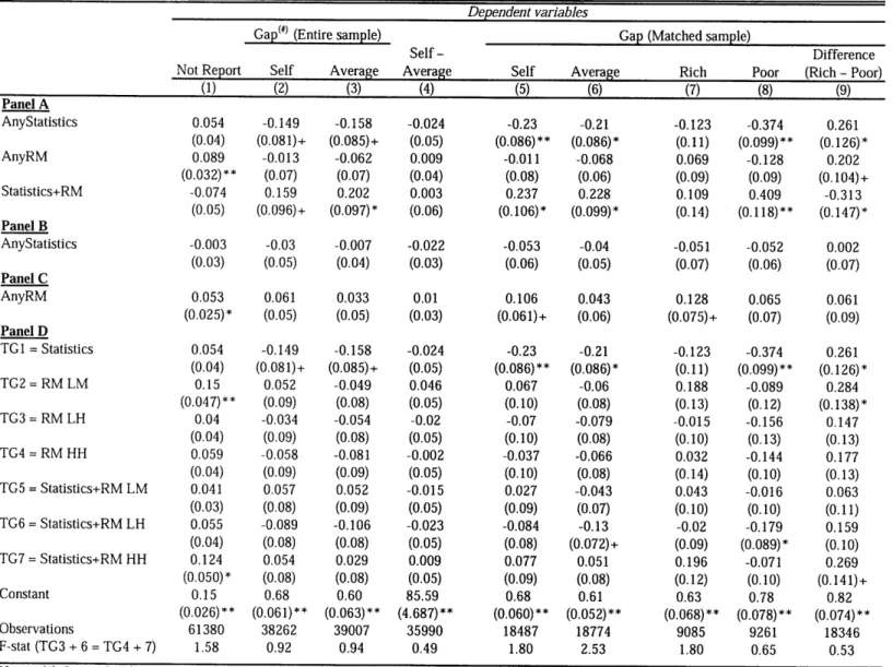
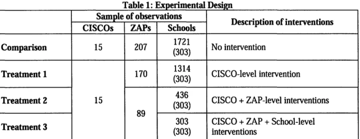
Table 1 describes the precise treatment design and distribution of program components. There are 8 treatment groups (TGO to TG7). The columns represent the "role model" interventions by type (TG2, TG3, and TG4 received a role model only). The second row represents the "statistics" intervention (TG1 received statistics only). I define "Any Statistics" as the second-row groups of 320 schools, and "Any RM" as the 480 schools in the last three columns. TG5, TG6, and TG7 refer to the combined treatment schools, who received both the statistics and role model treatments. In

8

Discussion on the statistics took place first to help mitigate the possibility that it might be overshadowed by the role models.

9

The AGEMAD packaged intervention provides (i) operational tools and training to administrators and teachers, (ii) report cards and accountability meetings with a purpose to improve the alignment of incentives. This cross-cutting design does not a priori restrict external validity since I do not expect any interactions between AGEMAD and the treatments explored in this paper. Indeed, when I test for this interaction, the treatment effects of statistics

all program schools, Grade 4 (aged 9-15) is the only treatment cohort. Other cohorts may have been indirectly affected since, for example, parents often have more than one child in the same primary school.

As mentioned earlier, the comparison group (TGO) still received the placebo meeting, but neither the statistics nor the role model interventions. Aside from the design table, 69 other schools were randomly chosen to be "pure control". Those schools did not come into contact with any announcement of the program, nor any baseline survey administered, nor any school meeting organized by the program. I will compare test scores in those schools (the only data available for this group) to those of the regular comparison group to detect any potential effect of simply participating in the experiment: answering survey questions and attending a meeting.

This evaluation design allows me to address the main questions in this paper concerning how individuals respond to information about the returns to education. First, TG1 versus TGO tells us to what extent providing pure statistical information changes one's perceived returns and schooling decisions. Second, I can measure whether role models are overall effective in changing behaviors, or only someone of the same type has a positive impact on effort. Third, the combined treatment schools help us understand what happens to the impact of statistics when extra information such as a role model is also presented.

1.4 Data and Experimental Validity

1.4.1

Data

1.4.1.1

Background Data

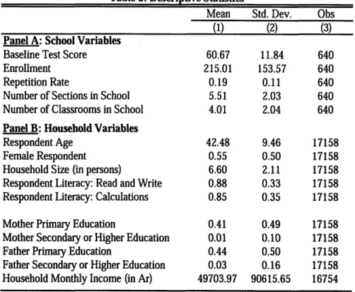
Background information on the schools is available from administrative data collected by the Min-istry of Education. In addition, I collected some information on household characteristics in a parent survey in all the schools of my sample. Table 2 presents descriptive statistics at baseline

for the sample of schools and households in this study. The average primary school has around 215 students in total enrollment for Grades 1-5, and 30 students in Grade 4. From the baseline test scores, the average student can reach 60% of the competency level they are expected to master. Their families are mostly poor, but I will refer to the top half of income as the relative "rich" in this sample. Less than half of the parents finished primary school, despite their high level of self-reported literacy.

1.4.1.2 Perception of Returns to Education

Evaluation of the statistics and role model interventions rests on three main data sources collected during the experiment: parent surveys, school attendance data, and Grade 4 students' test scores. The first one is subjective data on beliefs, while the latter two give objective measures of schooling. All data, except attendance, were collected for my entire sample at baseline (mid-school year) and ex-post (at the end of the school year). The actual sample turned out to be slightly fewer than 640 schools since some did not have Grade 4 during the study period.

I designed a parent survey to measure the first outcome of interest-perceived returns to educa-tion. This data allows us to gain a better understanding of the potential information gap at the household. At the beginning and the end of this project, surveyors visited the homes of Grade 4 students and interviewed either parent of the child (55% of the respondents were mothers). My survey approach follows Jensen (2007) and previous literature to elicit each individual's perceptions of the returns to education, both for the average and for oneself. We want to measure these two numbers since dispersion in perceived returns for oneself reflects both heterogeneity in the actual returns and possible misperception. Dispersion in perceived average returns, on the other hand, would reflect misperception (unless parents do not fully understand the survey question).

The exact survey question on perceived average earnings is as follows:

without a primary school degree"

The same question repeats for other scenarios of educational attainment. There are four scenar-ios in total: no primary education, only primary education, only lower-secondary education, and only high school education. Respondents also gave an estimate of their own child's (the Grade 4 student) income in hypothetical cases of various educational attainments, in response to two consecutive questions:

"Suppose, hypothetically, that your child were to leave primary school without ob-taining the CEPE [primary school degree] and not complete any more schooling. What types of work do you think he/she might (be offered and) choose to engage in when he/she is 25 years old?"

"How much do you think he/she will earn in a typical month at the age of 25?"

The answer to the first question is perceived job type by education. The answer to the second question is perceived earnings by education. From respondents' perceived earnings by education, I calculate the corresponding proportional gain in earnings due to education. I call this proportional gain "perceived returns to education." For each child, there are three levels of perceived returns: additional gain from primary education, lower-secondary education, and high school. For example, the perceived return to lower-secondary school is defined as

Perceived Earnings(Secondary) - Perceived Earnings(Primary) Perceived Earnings(Primary)

In this paper, I refer to respondents' estimates of the average returns as "perceived returns for average," and those of the child as "perceived returns for self." I measure for each individual at baseline his perceived returns for self and for average. Endline perceived returns to education is individual-level data, and is name-matched to the baseline perceived returns at 75% match rate.

1.4.1.3 Schooling Outcomes

Attendance rate is measured by the ratio of students present to total enrollment, at the school-grade level. This attendance data was collected by surveyors during unannounced school visits (one visit per school). It is available for only a random subset of schools in the study sample. This variable indicates whether the role model and statistics interventions entice students to exert more effort to attend school.

Lastly, I examine students' achievement through individual test scores. The baseline and post-tests measure children's competency in three materials: mathematics, French, and Malagasy. The baseline test took place in February 2006, and the post-test was administered to the same children (in Grade 4) in June 2007, as part of the AGEMAD project. Due to administrative constraints, only a random sub-sample of 25 students maximum per school took the test. These tests were developed from existing PASEC exams.10 They cover basic calculations and grammar questions in French and Malagasy, at the level that the students are supposed to master at this stage. These tests are achievement rather than ability tests, so performance can be improved by increasing effort. Test scores are calculated as the percentage of correct answers. Throughout the paper, I report test scores normalized by the control group mean and standard deviation for easier comparisons across different scales. Test score data is name-matched to the baseline perceived returns at 50% match rate.

1.4.2

Experimental Validity

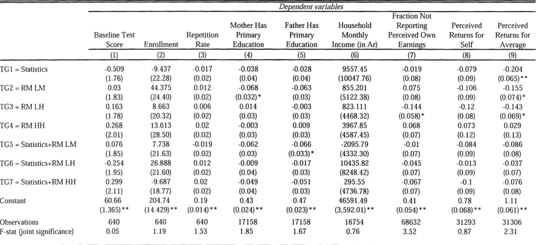
First, as expected given the randomized design, Table 3 shows that baseline test scores, school size, and repetition rate are statistically indistinguishable across the treatment groups and the comparison group. Columns 4 to 6 reassure that pre-existing differences in household data are mostly insignificant as well, with low point estimates. Only baseline perceived returns for average

'OPASEC (Programme d'Analyse des Systemes Educatifs de la CONFEMEN) is a program in 15 francophone countries that studies elements of learning for students.

seem to be different in the statistics and role model LM and LH groups.

Second, to minimize the potential bias caused by differential attrition, I tried to measure out-come variables for all the original participants of the program. Both the baseline and endline surveys were administered at the homes of the students just a few months apart. Any attrition is likely to be due to practical constraints of conducting the survey, such as unfavorable weather, rather than endogenous reasons related to the treatments themselves.

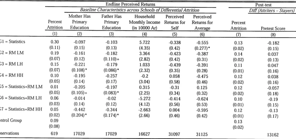
Column 1 of Table 4 presents mean attrition rates from the parent survey in all the treatment groups. While the statistics treatment schools have quite high attrition, the differences in mean attrition are not statistically significant. Columns 2 to 6 examine whether the differences in baseline characteristics of schools with high and low attrition vary across treatment groups. These columns report coefficient estimates from regressing each baseline characteristic on attrition rate interacted with treatment group dummies. Only parental education appears different for schools of different attrition rates across some treatment groups.

The post-test was administered to as many of the baseline children as possible. The school director had asked children who no longer attended school to come at the day of the test; and test administrators tried to find the absent students at home. As shown in column 7 of Table 4, attrition rate in test score data is around 0.12 and similar across treatment groups. Column 8 shows that pretest score differences between attriters and stayers are also similar across treatment groups, implying that attrition is not likely to be selected in terms of the pretest.

Due to time and budget constraints, attendance data is available for only a random sub-sample of 176 schools. While the small sample size prevents very precise estimation, there should not be any attrition bias since this sub-sample was randomly chosen.

1.5

Estimation Strategy and Results

The objective of this paper is first to understand better the distribution of initial perceived returns to education, and how perceived returns for self and for average compare to the estimated average return. Then, it examines the effects of statistics and different kinds of role models on perceived returns to education and schooling outcomes. I present the findings below in that order.

1.5.1

Baseline Perceived Returns to Education

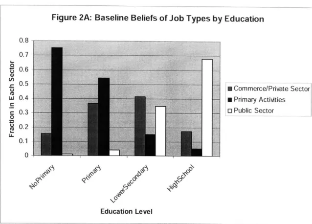
I exploit survey data on perceived jobs and perceived earnings as described in section 1.4.1.2. Figure 2A shows the fraction of the respondents who thought their children, with various education levels, would work in a certain sector. If everyone has the correct perception, these fractions should match the empirical job distribution. Most parents associate higher education with jobs in the public sector. In reality, only 33% of high school graduates work for the government while 40% work in commerce and the private sector, a sharp contrast from the beliefs shown in this figure.

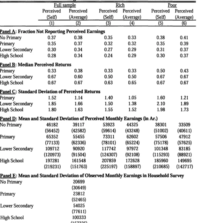
Answers to the survey question on perceived earnings reveal huge variation in parents' estimates of the returns at baseline. First, roughly one third of the respondents do not report perceived earnings, answering "Don't Know" to the survey question (even though almost everyone could predict the job type and report his household income). Panel A of Table 5 presents the fraction of the sample not knowing perceived earnings for self and for average at baseline. More respondents claim to know earnings for higher education, perhaps since they can perceive the standard salaries for public sector jobs but not the variable incomes in agriculture. The poor appear somewhat

more likely to answer "Don't Know" perceived earnings (also true for the less educated).

Second, conditional on knowing, perceived returns are dispersed; however, the median percep-tion is close to the estimated average return (Mincer estimates from household survey data). Figure 2B plots the kernel densities of the empirical distribution of perceived returns. The wide dispersion in perceived returns for self may reflect both heterogeneity in returns and imperfect information.

It is important to note that perception about the average returns also varies widely, revealing some extent of misperception. Differences between perceived return for self and that for average, i.e. an individual's relative position to the average, are mostly concentrated around zero.

Interestingly, in all cases, the median perceptions are well aligned with the estimated average returns. Despite large dispersion in perceived returns, the median of each distribution is quite close to the vertical line denoting the estimated average return in all the graphs of Figure 2B. Panels B and C of Table 5 report the median perceived returns and standard deviation. For example, the median person in the full sample thinks his marginal return to lower-secondary education is 0.67, i.e. 67% gain in income compared to completing just primary school. It is interesting to note that the poor have higher median perceived returns, though the standard deviation is also higher. These differences in perceived returns reflect underlying differences in perceived earnings. For all education levels, the poor's perceived earnings are consistently lower than those of the rich (see Panel D). Still, the poor expect to gain more from education. Poor people think they earn very little with lower education levels but can increase earnings substantially with higher education. The relatively rich people in my data think they can earn a fair amount even with little education. Third, dispersion in perception appears larger than dispersion in the actual earnings recorded in household survey data. Panels D and E of Table 5 display the mean and standard deviation of perceived and observed earnings. The mean perceived earnings are higher, which might be reasonable if parents already take into account growth and inflation in estimating children's earnings in the future. The standard deviation in perception is always larger than that in the survey data, for all levels of education. This evidence again suggests some extent of imperfect information about the returns to education.

1.5.2 Estimation Strategy

I first ask whether the statistics program as a whole has an impact on perception and schooling by pooling the "statistics only" and "statistics with role model" schools to be the "any statistics"

treatment. I ask the same question about the role model program as a whole. I also discuss the impact of statistics by itself, role model program by itself, and both interventions together. The main specifications are of the following form:

Ysi = a + "yo * AnyStat, + 6X,i + esi (1.22) Ysi = a + "y * AnyRM, + 6Xi + esi (1.23)

Ysi = a + "Y2 * AnyStat, + "73 * AnyRM, + 74 * StatRM, +

6Xi + esi

where Yi is an outcome variable for individual i in school s. AnyStat is a dummy equal to 1 if school s receives any statistics treatment, and similarly AnyRM for any role model treatment. StatRM is an indicator for the schools that received the combined interventions, i.e. the intersection of AnyStat and AnyRM. -y's are the coefficients of interest, to be interpreted as the average treatment effect. For example, Y2 in equation 1.24 is the difference between average Y in statistics (only) schools and that of the comparison schools. '2 + y3 + 74 is the effect of receiving both interventions relative to the comparison schools. Standard errors are clustered at the school level. Observations are weighted by the probability of selection, i.e. sampling weights, so that the coefficients of interest are estimated for the population. Xi refers to control variables in some specifications. In most cases, I control for the baseline value of the dependent variable, which is likely to have good explanatory power for the dependent variable and improve precision of the coefficient estimates.

For comparison and to evaluate the impact of role models by type, results from the complete specification of all treatment groups are also presented:

Ysi = + Ey k _{* TGk + 6Xsi + esi (1.25)}

k

where TGk are indicators for whether school s belongs to treatment group k (k=1 to 7) as defined in the design Table 1. Since treatment assignment was random, the errors esi are orthogonal to

treatment group dummies.

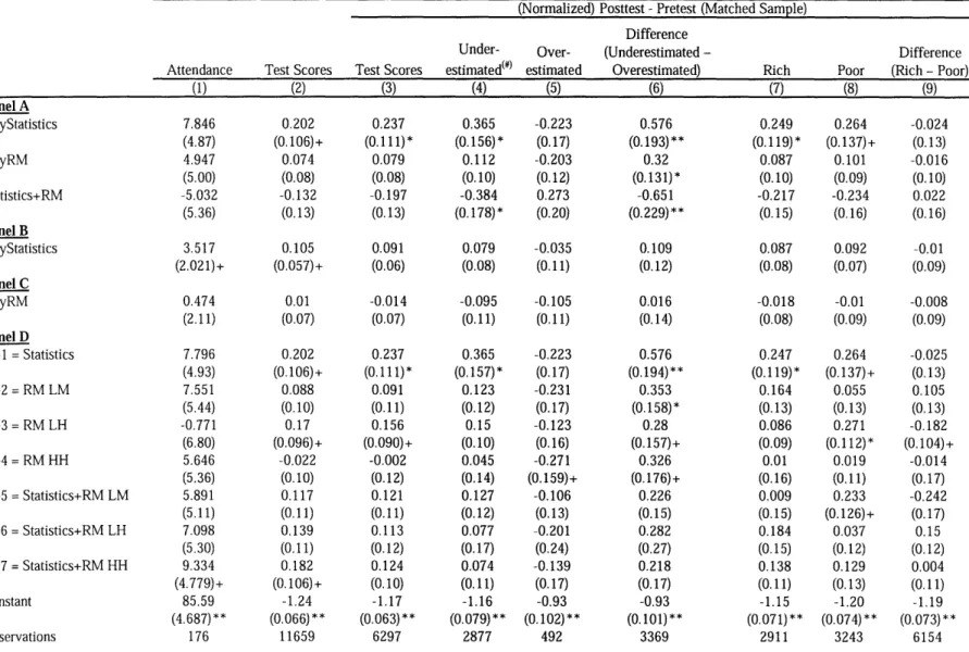
Motivated by the model's predictions, I also investigate the treatment effects by initial percep-tion and by type (rich vs. poor). In particular, any schooling improvement due to the statistics treatment should come from individuals whose initial perceived returns were below the estimated average returns (I call this "underestimate"). I test this prediction by running the following regression:

(Posttest - Pretest),i = a + yAnyStat, + ' 2AnyRM, + y3StatRM, + 5Pretest8i(1.26)

+AjAnyStat, 1l(Under),i + A2AnyRM, * 1(Under)si (1.27)

+A3StatRM, * 1(Under),i + 0 * l(Under) + ei (1.28)

where 1(under) is a dummy equal 1 if at baseline, the individual perceived the returns to be lower than the statistics provided. The coefficients of interest are A's on the interaction terms. A positive A would imply stronger treatment effects on those who had underestimated the returns. Moreover, we expect role model LH to increase the poor's schooling investment, but not the rich's. I run a regression similar to equation 1.26, with all the seven treatment dummies interacted with an indicator for (relatively) rich households. I will present these results in addition to the average treatment effects.

1.5.3

Impact on Perceived Returns

1.5.3.1

Impact of Statistics on Perceived Returns

I first discuss the impact of the statistics intervention on endline perception, as summarized in Table 6. The fraction of respondents not reporting perceived earnings decreased substantially from the baseline to the endline survey. Only 15% of respondents in the comparison group failed to report their perception (answering "Don't Know"), perhaps since the perception questions were