Eddy covariance fluxes and vertical concentration gradient measurements of NO and NO[subscript 2] over a ponderosa pine ecosystem: observational evidence for within-canopy chemical removal of NO[subscript x]

Eddy covariance fluxes and vertical concentration

gradient measurements of NO and NO[subscript 2] over

a ponderosa pine ecosystem: observational evidence

for within-canopy chemical removal of NO[subscript x]

The MIT Faculty has made this article openly available.

Please share

how this access benefits you. Your story matters.

Citation

Min, K.-E., S. E. Pusede, E. C. Browne, B. W. LaFranchi, and R.

C. Cohen. “Eddy Covariance Fluxes and Vertical Concentration

Gradient Measurements of NO and NO2 over a Ponderosa Pine

Ecosystem: Observational Evidence for Within-Canopy Chemical

Removal of NOx.” Atmospheric Chemistry and Physics 14, no. 11

(2014): 5495–5512.

As Published

http://dx.doi.org/10.5194/acp-14-5495-2014

Publisher

Copernicus GmbH on behalf of the European Geosciences Union

Version

Final published version

Citable link

http://hdl.handle.net/1721.1/89165

Terms of Use

Creative Commons Attribution

www.atmos-chem-phys.net/14/5495/2014/ doi:10.5194/acp-14-5495-2014

© Author(s) 2014. CC Attribution 3.0 License.

Eddy covariance fluxes and vertical concentration gradient

measurements of NO and NO

2

over a ponderosa pine ecosystem:

observational evidence for within-canopy chemical removal of NO

x

K.-E. Min1,*, S. E. Pusede2, E. C. Browne2,**, B. W. LaFranchi2,***, P. J. Wooldridge2, and R. C. Cohen1,2

1_{University of California at Berkeley, Department of Earth and Planetary Science, Berkeley, USA} 2_{University of California at Berkeley, Department of Chemistry, Berkeley, USA}

*_{now at: NOAA Earth System Research Laboratory and Cooperative Institute for Research}

in Environmental Sciences, University of Colorado, Boulder, USA

**_{now at: Department of Civil & Environmental Engineering, Massachusetts Institute of Technology, Cambridge, USA} ***_{now at: Lawrence Livermore National Lab, Center for Accelerator Mass Spectrometry (CAMS), Livermore, USA}

Correspondence to: R. C. Cohen (rccohen@berkeley.edu)

Received: 8 April 2013 – Published in Atmos. Chem. Phys. Discuss.: 14 May 2013 Revised: 16 March 2014 – Accepted: 22 April 2014 – Published: 4 June 2014

Abstract. Exchange of NOx(NO+NO2)between the

atmo-sphere and bioatmo-sphere is important for air quality, climate change, and ecosystem nutrient dynamics. There are few di-rect ecosystem-scale measurements of the didi-rection and rate of atmosphere–biosphere exchange of NOx. As a result, a

complete description of the processes affecting NOx

follow-ing emission from soils and/or plants as they transit from within the plant/forest canopy to the free atmosphere remains poorly constrained and debated. Here, we describe measure-ments of NO and NO2fluxes and vertical concentration

gra-dients made during the Biosphere Effects on AeRosols and Photochemistry EXperiment 2009. In general, during day-time we observe upward fluxes of NO and NO2with

counter-gradient fluxes of NO. We find that NOxfluxes from the

for-est canopy are smaller than calculated using observed flux– gradient relationships for conserved tracers and also smaller than measured soil NO emissions. We interpret these differ-ences as primarily due to chemistry converting NOxto higher

nitrogen oxides within the forest canopy, which might be part of a mechanistic explanation for the “canopy reduction fac-tor” applied to soil NOxemissions in large-scale models.

1 Introduction

The chemistry of nitrogen oxides is a major factor affect-ing the oxidative capacity of the atmosphere and the global burden of tropospheric ozone (Crutzen, 1973). Reactive ni-trogen oxides are also a nutrient (Sparks, 2009; Takahashi et al., 2004, 2005a; Teklemariam and Sparks, 2004; Lockwood et al., 2008) and interactions between available nitrogen in ecosystems and atmospheric nitrogen are many and com-plex, with exchange processes altering the patterns of nitro-gen availability in the biosphere (Townsend et al., 1996; Vi-tousek and Farrington, 1997; ViVi-tousek et al., 1997; Holland and Lamarque, 1997; Holland et al., 1997; Ollinger et al., 2002a, b; Hietz et al., 2011). Nitrogen is the limiting nutrient for plant growth in most regions outside the tropics (Hungate et al., 2003; Galloway et al., 2004; Hietz et al., 2011), thus nitrogen deposited to the surface after atmospheric trans-port can act as fertilizer contributing to enhanced carbon up-take (H. Morikawa et al., 2004; T. Morikawa et al., 2004; Takahashi et al., 2004, 2005a, b; Sparks, 2009; Norby et al., 2010). For example, Norby et al. (2010) found that the avail-ability of nitrogen was a major limiting factor for the CO2

fertilization effect in the FACE (Free-Air CO2Enrichment)

experiment. However, excess nitrogen deposition may im-pair ecosystem health (Hessen et al., 1997; Herman et al., 2001) by causing dehydration, chlorosis, or membrane dam-age from peroxy acetal nitrate (PAN) (Ordin et al., 1971;

Oka et al., 2004), or by inducing soil acidification and eu-trophication (Makarov and Kiseleva, 1995; Pawlowski, 1997; Gbondo-Tugbawa and Driscoll, 2002; Zapletal et al., 2003; Chen et al., 2004).

A comprehensive understanding of NOx exchange

be-tween the atmosphere and biosphere does not yet exist. Ex-perimental studies have primarily focused on NO emissions from soils to the atmosphere (e.g., Butterbach-Bahl et al., 2002; Gasche and Papen, 2002; Gut et al., 2002a, b; Rummel et al., 2002; van Dijk et al., 2002; Dorsey et al., 2004; Duyzer et al., 2004; Feig et al., 2008; Bargsten et al., 2010; Yu et al., 2010) or on the leaf-level transfer of NO and NO2

us-ing branch enclosures (Hereid and Monson, 2001; Chaparro-Suarez et al., 2011; Breuninger et al., 2013; and references therein). Studies at the canopy-scale often assume a sim-ple flux–gradient similarity relationship, meaning molecu-lar movement is always along the gradient of high to low concentration, to infer the rate of exchange from vertically resolved observations (Mayer et al., 2011 and references therein). Direct measurements of the direction and rate of exchange (the flux) at the canopy scale are few (Wesely et al., 1982; Wildt et al., 1997; Horii, 2002, 2004; Farmer et al., 2006; Neirynck et al., 2007; Li and Wang, 2009; Brummer et al., 2013).

The base conceptual model for biosphere–atmosphere ex-change of NOx is shown in Fig. 1. In this model, NO is

mainly emitted by soil microbial activity, is converted to NO2

by reaction with O3, and is then ultimately oxidized to nitric

acid (HNO3), which returns back to the biosphere via wet

and dry deposition. The timescale of NO to NO2conversion

by O3 and the photolysis of NO2 back to NO is typically ∼100 s in the daytime, set by the photolytic and chemical re-action rates, and is comparable to the turbulent mixing time (τturb)within and out of a forest canopy. The timescale for

NOxoxidation to HNO3via reaction of OH with NO2is 3–

10 h, long enough that NOxchanges by less than 1 % on the

canopy residence timescale from this loss process. The rapid interconversion between NO and NO2implies that the

indi-vidual fluxes of NO or NO2will not follow the form of fluxes

of a conserved tracer, such as water, heat, or carbon dioxide (Vila-Guerau de Arellano et al., 1993), but the long lifetime of the sum implies the flux of NOx, will follow that of

con-served tracers.

This model of NOx exchange is qualitatively supported

by ecosystem-scale observational studies. For example, NO is observed to decrease as air is transported up through a canopy from the forest floor (e.g., Rummel et al., 2002) and the low light levels within a shaded canopy reduce NO2

pho-tolysis and enhance the NO2to NOxratio. For these reasons,

downward NO fluxes and upward NO2fluxes in across the

canopy top at Harvard forest have been observed as expected (e.g., Horii, 2002).

Calculations of ozone by large-scale chemical transport models parameterized with measured NO soil fluxes over-predict O3concentrations in comparison to aircraft and tower

observations (e.g., Lerdau et al., 2000). To match obser-vations, these models invoke a canopy reduction factor of 25–80 % (Jacob and Wofsy, 1990; Yienger and Levy, 1995; Wang and Leuning 1998). This parameter removes soil NOx

exclusively before it escapes the canopy, thus preventing its contribution to atmospheric ozone formation. Typical param-eterizations use LAI (leaf area index) and SAI (stem area in-dex) as parameters controlling the removal of soil NOx. To

our mind these mechanisms are unphysical as they do not act on all NOxin the plant canopy – but only on soil NOx. One

motivation for our experiment is to quantify NOx removal

processes in order to develop a physically based model that treats all NOxidentically regardless of source.

At the same time, laboratory observations at the leaf scale indicate bi-directional exchanges of NOx by plant biota,

where the direction and rate of exchange is controlled by a so-called “compensation point” – a concentration above which vegetation takes up NO2and/or NO but below which

emissions occur (Sparks et al., 2001; Raivonen et al., 2009; Chaparro-Suarez et al., 2011; Breuninger et al., 2013); how-ever, a mechanism for the emissions remains to be discovered (Breuninger et al., 2013). Direct observations of the NO2

compensation point are analytically challenging (Raivonen et al., 2003) and evidence suggests that compensation behav-ior is not fixed but rather varies by plant species, plant life cycle, and environmental conditions (Raivonen et al., 2009). That said, compensation points have been measured in the range of ambient NO2 abundances and have been reported

from 0.05 to 3 ppb (Sparks et al., 2001; Raivonen et al., 2009; Chaparro-Suarez et al., 2011; Breuninger et al., 2013). Since the NO2concentration in remote continental regions is

typi-cally less than 1 ppb, these observations leave open the pos-sibility that the majority of forests on earth are a source of NOxfrom direct NO2emissions from plants, in addition to

any soil NO emissions. This is in direct contradiction with the need for canopy reduction factors that remove nitrogen oxides emitted from soils prior to its exit from plant canopies (Lerdau et al., 2000).

Recent field studies suggest the existence of rapid within-canopy chemistry affecting nitrogen oxides that is not included in the conceptual model of Fig. 1. Farmer et al. (2006) observed upward exchanges of total peroxynitrates (6RO2NO2) and HNO3 and interpreted this as the

forma-tion of these molecules within a forest canopy. In addiforma-tion, Wolfe et al. (2009) described the importance of chemical pro-cesses in speciated acyl peroxynitrate exchange, also find-ing observational evidence for within-canopy chemistry af-fecting observed fluxes. Several other experimenters have reported the occurrence of within-canopy chemistry affect-ing fluxes of biogenic volatile organic compounds (BVOCs) (Holzinger et al., 2005; Karl et al., 2005; Bouvier-Brown et al., 2009a, b; Park et al., 2014) and ozone (Kurpius and Gold-stein, 2003). Our own recent study of peroxynitrate fluxes (Min et al., 2012) supports this idea, providing experimen-tal evidence for upward fluxes of unidentified peroxynitrates

(FXPN) formed within the forest canopy. Taken together,

these studies emphasize the importance of rapid chemistry not only for determining the magnitude but also for the direc-tion of nitrogen exchange at the biosphere–atmosphere inter-face.

The Biosphere Effects on AeRosols and Photochemistry EXperiment (BEARPEX) included a component designed to provide comprehensive measurements of vertical concentra-tion gradients and fluxes of a wide suite of nitrogen oxides – NO, NO2, total and speciated peroxynitrates, total and

speci-ated alkyl (6RONO2)and multifunctional nitrates, HNO3,

and nitrous acid (HONO) – and therefore presented a di-rect opportunity to test our ideas about canopy-scale NOx

exchange. Analyses of peroxynitrate (Wolfe et al., 2009; Min et al., 2012) and HONO (Ren et al., 2011) fluxes have been reported elsewhere. Here we present observations of vertical concentration gradients and fluxes of NO2 and NO

measured with laser-induced fluorescence and chemilumi-nescence, respectively. Fluxes are derived using the eddy co-variance method. We describe relationships between gradi-ents and fluxes, present and interpret evidence for chemi-cal canopy reduction processes, and explore the significance of chemistry within the canopy to the import/export of NOx

from the canopy.

2 Research site and instrumentations

The data used in this work were obtained as a part of the BEARPEX 2009 experiment (15 June–31 July 2009). The experiment was conducted over a managed Pon-derosa pine plantation on the western slope of the Sierra Nevada Mountain range, 75 km downwind of Sacra-mento, California and near the University of Califor-nia Berkeley Blodgett Forest Research Station (UC-BFRS, 38◦53042.900N, 120◦3757.900W; 1315 m). Many of the re-sults from BEARPEX can be found in a special is-sue of Atmospheric Chemistry and Physics, http://www. atmos-chem-phys-discuss.net/special_issue89.html. A brief description of the field site and of the instrumentation rele-vant to this paper follows.

Analysis of the local meteorology by Choi et al. (2011) and Dillon et al. (2002) indicate that in the summer (May– September), winds at the BEARPEX site are characterized by daytime southwesterlies (210–240◦) and nighttime north-easterlies (30◦_{) with little variability. The major source of}

anthropogenic emissions in the region is the city of Sacra-mento and its suburbs. There is a line source of oak trees that are strong isoprene emitters aligned perpendicular to the flow between the urban center and the site. This source distribu-tion, in combination with the regular winds, results in low concentrations of trace gases with anthropogenic or isoprene sources early in the morning and higher concentrations in air transported from the west later in day (Dillon et al. 2002; Day et al., 2003; Murphy et al., 2007; Choi et al., 2011; LaFranchi

et al., 2011). The two sources arrive at distinct times; with air influenced primarily by isoprene arriving at approximately noon and the urban plume combined with the isoprene source arriving about 3–4 h later.

There were two sampling towers at the site: a 15 m walk-up tower on the south side of the site (hereafter south tower) and an 18 m scaffolding tower located 10 m north of the south tower (hereafter north tower). On the south tower, tem-perature, relative humidity, wind speed, net radiation, pho-tosynthetically active radiation (PAR), water vapor, carbon dioxide (CO2), and O3 were monitored at 5 heights (1.2,

3.0, 4.9, 8.75, and 12.5 m above the forest floor). At 12.5 m, fluxes of water vapor, CO2, and O3 were measured.

Ver-tical gradients of temperature, relative humidity, and wind speed were also measured on the north tower at 5 heights (1.2, 5.4, 9.2, 13.3, and 17.5 m above the forest floor). Mea-surements from the north tower or on an adjacent height-adjustable lift included NO, NO2, HONO, total peroxy

ni-trates (6PNs, RO2NO2), total alkyl and multifunctional

ni-trates (6AN, RONO2), HNO3, hydroxyl radical (OH),

hy-droxy peroxy radical (HO2), OH reactivity, O3, several

in-dividual PNs, several inin-dividual ANs, numerous volatile or-ganic compounds (VOCs) including many biogenic VOCs (BVOCs), formaldehyde (HCHO), glyoxal, methylglyoxal, organic peroxides, and aerosol chemical and physical prop-erties. Needle temperature, soil moisture, soil temperature, and soil heat flux were also monitored. All measurements were made at the 17.5 m level and many were additionally recorded at one or more of the following heights: 0.5, 1.2, 5.4, 9.2, and 13.3 m. For simplicity, we refer to these mea-surement heights as 0.5, 1, 5, 9, 13 and 18 m. In addition, soil NO measurements were made using dynamic chambers on 2 July (09:15, 13:40 and 18:10), 12 (08:25 and 16:20) and 30 (08:50 and 16:10) to provide an observational constraint on the soil NO emission at this site: soil NO flux from four different locations (15 min sampling each) were measured to represent morning, midday and the late afternoon time win-dow.

The upper canopy at this site was mainly Pinus pon-derosa L., with a few scattered Douglas fir, white fir, and incense cedar. The understory was primarily moun-tain whitethorn (Ceanothus cordulatus) and manzanita (Arc-tostaphylos species) shrubs (see Misson et al., 2005, for a more detailed site description and history). The mean tree height was 8.8 m and the leaf area index (LAI) was 3.7 m2m−2_{, based on a tree survey conducted on}

17 July 2009.

NO was measured using a custom-built two-channel chemiluminescence NO detection system (2ch-CL) and NO2

with two separate thermal-dissociation laser-induced fluores-cence (TD-LIF) systems. The sampling inlets for NO and NO2 were collocated at 0.5, 5, 9 and 18 m on the north

tower and represent the forest floor, mid-canopy, top canopy, and above canopy, respectively. At 18 m, fluxes of NO and NO2were monitored along with 3-D wind and temperature

Figure 1. Schematic of the various interactions involved in the exchange of nitrogen oxides between the atmosphere and the forest canopy.

Bold arrows in blue (downward) and red (upward) represent the direction of the flux of each species across the canopy surface.

from a sonic anemometer (Campbell Scientific CSAT3 3-D Sonic Anemometer). The measurements were combined to infer fluxes using an eddy covariance method (EC) (see Sect. 3). The sonic anemometer was pointing into the mean daytime wind stream with 0.02 m vertical displacement and 0.2 m horizontal displacement from the NO and NO2inlets.

The 2ch-CL system for the NO flux and vertical gradient measurements was based on the standard O3

chemilumines-cence method. A detailed description of the operating prin-ciple can be found elsewhere (Drummond et al., 1985 and references therein). Briefly, ambient NO is combined with an excess of O3generated by electric discharge in O2. The

re-action of NO and O3produces excited-state NO2molecules,

which then fluoresce. Two gold-plated detection cells were used for simultaneous flux and vertically resolved concen-tration measurements. The signals from photocathodes (flux channel: EMI 9658B, gradient channel: Hamamatsu H7421-50) were acquired at 5 Hz. The cell pressures were main-tained at 8–8.7 Torr with pressure restricted at the inlet and a fluorinated oil-sealed rotary vane pump. During the sampling mode, 100 % of the ozone flow was added directly into the detection cell to monitor the ambient NO concentration (for 24 s). The background signal was monitored by adding 50 % of the O3 to the sampling air prior to the detection cell to

titrate ∼ 90 % NO (for 6 s). Incomplete titration of NO was employed to limit interferences from fluorescence of vibra-tionally excited OH molecules produced in the reaction of ozone with alkenes (Drummond et al., 1985). The other 50 % of the ozone was added directly to the cell to minimize flow changes within the reaction cell between the sampling and the background mode. Our own laboratory experiments con-firm that a wide variety of terpenes react with ozone to effi-ciently produce vibrationally excited OH and we configured the instrument to minimize detection of this signal.

Two TD-LIF systems were used for simultaneous flux and vertical gradient measurements of NO2and the higher

nitro-gen oxide species 6PNs, 6ANs and HNO3. Details of LIF

detection of NO2(Thornton et al., 2000), thermal

dissocia-tion of higher nitrogen oxides (Day et al., 2002), and

appli-cation to EC flux measurement (Farmer et al., 2006) are de-scribed elsewhere. Briefly, thermal dissociation of each class of higher oxide generates NO2and a companion radical at the

characteristic temperatures ∼ 180◦C for 6PNs, ∼ 350◦C for

6ANs, and ∼ 600◦C for HNO3, (Day et al., 2002). The

ther-mal dissociation is followed by detection of NO2by LIF. In

both TD-LIF systems, excitation at 585 nm was provided by frequency doubled Nd:YAG (Spectra Physics, average power of 2 W at 532 nm, 30 ns pulse length) pumping a custom-built tunable dye laser operating at 8 kHz. The wavelength of the dye laser beam was tuned to a specific, narrow rovibronic feature of NO2 by rotating an etalon within the dye cav-ity. We alternated the laser frequency between a strong NO2

resonance (8 s) and the weak continuum adsorption (4 s) to maintain a frequency lock on the spectral feature of interest. By adapting a supersonic expansion technique, we acquired

∼10-fold higher sensitivity to NO2 (Cleary et al., 2002).

The fluorescence signal 700 nm long was collected and im-aged onto a red sensitive photocathode (Hamamatsu H7421-50). Gated photon counting techniques (Stanford Research Systems, SRS 400) were employed to discriminate against prompt background signals. Laboratory measurements and comparison in the field showed the two TD-LIF instruments to have calibrations that were identical to within 4 % (slope: 1.0 ± 0.10, R2: 0.92). Allowing the intercept to vary from zero did not change the slope or R2.

Cell pressures in the flux system were reduced to 0.17– 0.19 Torr to achieve the high expansion ratios for the su-personic jet cooling by using Lysholm twin screw blowers (Whipple model 2300 superchargers) backed by an oil-sealed rotary vane pump. The jet nozzles and this pump system combined to maintain a 580–700 sccm flow through each of the four cells (total flow of 2300 sccm). To reduce high fre-quency damping of turbulent eddies and interference from secondary chemistry in the heated section of the inlet and sampling lines (30 m), we added a diaphragm bypass pump and maintained the total flow of a 13 000 sccm. For the gradi-ent system, critical orifices as pressures restrictors (AirLogic, F-2815-251-B85, 0.025” orifice diameter) were placed at the

39

1

2

Figure 2. Data collection scheme for fluxes of NO (a: 2ch-CL) and NO

(b: TD-LIF) and

3

vertical gradient (c) measurements. Colors represent the different measurement heights: 18m

4

(black), 9m (blue), 5m (green), and 0.5m (gray). Yellow periods are calibration cycles and

5

white periods represent times when diagnostics were collected.

6

7

Figure 2. Data collection scheme for fluxes of NO (a: 2ch-CL) and NO2(b: TD-LIF) and vertical gradient (c) measurements. Colors represent the different measurement heights: 18 m (black), 9 m (blue), 5 m (green), and 0.5 m (gray). Yellow periods are calibration cycles and white periods represent times when diagnostics were collected.

end of the inlet manifold to reduce the pressure along the sampling line.

Calibrations in the field were repeated once (gradient mea-surement of NO and NO2and flux measurement of NO) or

twice (flux measurement of NO2)per hour. NO2 standard

gas (4.9 ± 0.2 ppm Noxin N2, PRAXAIR) was diluted to 3–

20 ppb in zero air and added to system at the inlet tip. For NO, 2.25–6.7 ppb of NO (5.4 ppm ± 5 % NO in N2,

PRAX-AIR) was diluted with zero air and added at the inlet. Both cylinders were referenced to a library of calibration stan-dards maintained in our laboratory. The mixing ratios were corrected (< 2 %) for quenching by water using north tower RH measurements. To evaluate the background counts due to cell scatter and photocathode dark noise, we flowed excess zero air into the inlet once/twice per hour. The diagnostics for the NO and NO2flux instruments (calibration and

zero-ing) were completed within the first 3 min of every 30 min (Fig. 2a). Flux data for both species were collected at 18 m during the first 27 min, from the 3 to the 30 min, and for the last 27 min, from the 33 to the 60 min each hour (Fig. 2a). NO and NO2at the lower levels were measured by

switch-ing between the 9, 5, and 0.5 m heights and samplswitch-ing at each height for 2 min (Fig. 2b); the first 5 s for data of each level after the valve switching from another height were deleted to insure the measurement corresponded to the height in ques-tion. Calibrations and zeros were completed in the last 4 min from 56 to 60 min of every hour for both gradient systems (Fig. 2b).

Data affected by exhaust plumes from a nearby propane electrical generator (mostly at night) and the infrequent wafts of car exhaust were removed prior to analysis. These spikes were defined as variations in the NO or NO2 concentration

in excess of 3 times the standard deviation of the 10 min run-ning mean. A few remairun-ning spikes were identified through correlations with CO and removed by hand. Over the cam-paign, the NO2 detection limit (defined as S/N = 2) was ∼45 ppt for 1 s corresponding to 1.3 ppt for a 30 min av-erage for the flux system, and was ∼ 10 ppt 1 min (4.0 ppt for 30 min) for the gradient system. The NO detection limit for flux cell was ∼ 58 ppt for 1 s (1.6 ppt for 30 min aver-ages) and for the gradient cell, ∼ 29 ppt for 1 min (11.5 ppt for 30 min averages) at midday (12:00–14:00, local time).

3 Eddy covariance calculation

The flux (Fc)of an atmospheric constituent (c) (i.e., the

tur-bulent mass transport of c through a vertical reference layer) can be evaluated from the covariance between the concen-tration of c and the vertical wind (w) in a method known as eddy covariance (EC) and is represented mathematically by Eq. (1) (e.g., Foken, 2006; Lee et al., 2004; McMillen, 1988).

Fc= t Z t0 w0c0dt =1 n n X i=1 (wi−w)(ci−c) = w0c0 (1)

In Eq. (1), primes represent the deviation from the mean, subscripts i refer to individual high-time resolution measure-ments (NO or NO2), and bars indicates the mean over the

averaging interval. In this work, the flux of NOx, FNOx, is de-fined as the sum of the separately calculated FNOand FNO2. We checked this calculation by comparing with FNOx, cal-culated by first adding the NO and NO2concentrations and

found the two methods agree to within 18 %, which is smaller then propagated errors of FNOx estimated (Table 1) from the sum of FNOand FNO2.

We used 5 Hz data for the flux calculations and aver-aged for ∼ 30 min, a timescale that spanned the range of the major flux-carrying eddies at this site (e.g., Wolfe et al., 2009; Farmer et al., 2006). Prior to calculating fluxes, we rotated the wind measurements to ensure that the vertical winds were normal to the shear plane (Baldocchi et al., 1988; McMillen, 1988). We also de-spiked and de-trended the con-centration data, where spikes were defined as data greater than 3 times the standard deviation of the 10 min running mean, and where the 10 min running mean was also used for de-trending.

To synchronize the timing of wind and concentration measurements, the lag was determined from the maximum in covariance of the deviation from the mean of vertical wind speed and concentration; the cross-correlation between scalar and vertical wind were calculated for every 30 min and then averaged with multiple time windows (i.e., morn-ing: 10:00–12:00, midday: 12:00–14:00, afternoon: 14:00– 16:00) to determine the precise lag time. We did not find any

Table 1. Estimated flux analysis errors.

Source of error FNO FNO2 FNOx

Systematic error Data acquisition scheme < 2 % < 3 % < 4 %

(unbiased) (unbiased) (unbiased)

Sensor separation and <2 % <2 % <3 %

High frequency damping (underestimated) (underestimated) (underestimated)

Instrumental response time < 0.2 % < 0.7 % < 0.7 %

(underestimated) (underestimated) (underestimated)

Absolute concentration estimation < 7 % < 5 % < 9 %

(unbiased) (unbiased) (unbiased)

Total < 8 % < 6 % < 10 %

Random error Instrument noisea < 20 % < 10 % < 23 %

(unbiased) (unbiased) (unbiased)

Detection limit conceptb < 25 % < 21 % < 33 %

(unbiased) (unbiased) (unbiased)

a_{Errors over half an hour.}b_{Estimated form the ratio of covariances at true lag and several lag times far from the true lag (±230–250 s).}

40 1 -200 0 200 -0.5 0 0.5 1 1.5  [sec] C o rr e la ti o n (a) -200 0 200 -0.5 0 0.5 1 1.5  [sec] (b) -200 0 200 -0.5 0 0.5 1 1.5  [sec] (c) 2

Figure 3.Lag calculation of (a) w’T’, (b) w’NO’ and (c) w’NO2’. Highest normalized 3

correlation between wind and temperature, NO or NO2 were observed as expected; 0 second 4

for wind and temperature, 1.4 and 2.6 second for NO and NO2. 5

6

Figure 3. Lag calculation of (a) w0T0, (b) w0NO0and (c) w0NO0₂. Highest normalized correlation between wind and temperature, NO or NO2were observed as expected; 0 s for wind and temperature, 1.4 and 2.6 s for NO and NO2.

change in lag time with time of day. We compared the lag times in the different periods of the experiment and found no drift over the duration of the experiment. Three periods were tested, 18–30 June, 1 –15 July and 16–30 July, and each calculated lag time agreed within 1 data point (0.2 s) for both NO and NO2. Figure 3a–c show the lag correlation

between wind and temperature, NO, and NO2, respectively.

The data plotted in Fig. 3 are the averaged midday (12:00– 14:00) lag over the whole field campaign and are represen-tative of lag correlation plots throughout the experiment. As expected, zero lag was observed between vertical wind speed and temperature as both quantities are synchronously mea-sured by the same instrument, the sonic anemometer. Lag times for NO and NO2 were measured to be 1.4 and 2.6 s,

times that were consistent with transport times in the tubing (< 0.8 s) plus the time difference between sonic anemometer computer and computers for 2ch-CL and TD-LIF.

To assure that each 30 min flux was representative of the average surface exchange over the sampling period, we tested the calculated fluxes for stationarity (Farmer et al., 2006; Fo-ken 2006; Wolfe et al., 2009). To do this, five equally di-vided subsets of each 30 min flux period, Fsub, were averaged

and compared with that of the full period, F30 min. If Fsub

differed from F30 min by more than 30 % then that

measure-ment period was defined as non-stationary and that half-hour excluded from further analysis (Foken and Wichura, 1996). Also, the calculated flux data with a tilt angle greater than 5◦ from the wind rotation (Lee et al., 2004) and with a friction velocity smaller than 0.1 m s−1or larger than 1.5 m s−1 (Fo-ken 2006) were excluded for further analysis. We tested this using friction velocity in the range 0.05–0.2 m s−1as filter-ing criteria. Changes in this range do not affect our conclu-sion, which is consistent with previously reported analyses of fluxes at this site (Farmer et al., 2006).

Approximately 2/3 of the daytime and half of the night-time data remained after application of these filters. We es-timate the total uncertainty in FNOx by combining the sys-tematic and random error terms in FNOand FNO2 flux esti-mations following Moore et al. (1986) and Massman (1991). Each of the individual elements is summarized in Table 1 and detailed procedures are described in Farmer et al. (2006) and Wolfe et al. (2009).

The total systematic uncertainties for FNOand FNO2 (< 8 and < 6 %, respectively) are calculated from the root mean square of errors from instrument calibration (7 and 5 % for NO and NO2, respectively; see Day et al., 2002), sensor

separation and inlet dampening (< 2 % for both FNO and FNO2), instrument time response (< 0.2 % and < 0.7 % for daytime FNO and FNO2, respectively) and data acquisition sequencing (i.e., laser line-locking cycling for TD-LIF tem: < 3 % or frequent background checking for 2ch-CL sys-tem: < 2 %, estimated from the sensible heat flux calculation

41 10-2 10-1 100 10-8 10-6 10-4 10-2 100 Frequency [ Hz ] C o s p e c tr a l D e n s it y (a) wT s wNO₂ wNO wNO X f-7/3 f-5/3 10-2 10-1 100 0 0.05 0.1 0.15 0.2 0.25 Frequency [ Hz ] N o rm a li ze d c o s p e c tr u m (b) 10-2 10-1 100 0 0.1 0.2 0.3 0.4 0.5 0.6 0.7 0.8 0.9 1 Frequency [ Hz ] C u m u la te iv e C o s p e c tr u m (c) 1

Figure 4.Equally spaced logarithmic averaged (150 bins) absolute cospectral density (a), 2

frequency weighted cospectrum (b), and normalized cumulative distributions of the cospectra 3

of temperature (magenta) NO (green), NO2 (blue) and NOX (yellow) (c) with vertical wind

4

from 11:00-12:00 through out the whole field campaign when the chemical perturbation is 5

small. Closed triangles represent the absolute value of the negative cospectral density, which 6

has the opposite sign to the general flux direction. The black dotted lines in (a) are lines with 7

slopes of −7/3 and −5/3 (see related text). 8

9

Figure 4. Equally spaced logarithmic averaged (150 bins) absolute cospectral density (a), frequency weighted cospectrum (b), and

normal-ized cumulative distributions of the cospectra of temperature (magenta) NO (green), NO2(blue) and NOx(yellow) (c) with vertical wind from 11:00–12:00 through out the whole field campaign when the chemical perturbation is small. Closed triangles represent the absolute value of the negative cospectral density, which has the opposite sign to the general flux direction. The black dotted lines in (a) are lines with slopes of −7/3 and −5/3 (see related text).

using temperature data coincident with the NO or NO2data.

The gaps in the data acquisition sequence are replaced by the mean concentration for 27 min.)

Two different methods were used to estimate the preci-sion (random errors) of the flux measurements: (1) estimates based on the finite precision of photon counting and (2) the variance of the flux calculation with lag determination. The precision estimates based on photon-counting statistics fol-low Farmer et al. (2006) and are 0.08 ppt m s−1 (20 %) and 0.14 ppt m s−1(10 %) for FNO and FNO2, respectively, over half an hour. This estimate is similar to but slightly smaller than the precision of 25 % (0.10 ppt m s−1for FNO)and 21 %

(0.29 ppt m s−1 for FNO2)estimated from the flux variance over a range of lag times far from the true lag (Ruuskanen et al., 2011), indicating the presence of other sources of random error in the measurement in addition to photon counting. One common measure of the flux detection limit is 2 times the standard deviation of the covariance within the time window far from the peak covariance. We use ±230 ∼ 250 s during the daytime (09:00–18:00) (Table 1). The value is not signif-icantly different if we use smaller time windows. For cases such as ours, where fluxes are bi-directional, an alternative approach to estimating a detection limit based on the absolute cross-correlation has been proposed by Park et al. (2013). By either metric the fluxes we report are well above the noise.

Spectral analyses of the fluxes are shown in Fig. 4 and in-clude the cospectral density (Fig. 4a), the normalized cospec-trum (Fig. 4b), and the absolute value of the normalized cu-mulative cospectrum (Fig. 4c) for temperature, NO, NO2and

NOx. We show each measurement averaged for the time

in-terval 11:00–12:00 throughout the whole field campaign. By analyzing the NOx(yellow) cospectrum, rather than the

spec-tra of NO (green) and NO2(blue) separately, we are

insensi-tive to the effects of the rapid chemical conversion between NO and NO2. The absolute values of the negative cospectral

density were plotted as closed triangles in Fig. 4. The figures show that we capture the full range of eddies that contribute to the flux.

The spectral analysis of NOxprovides additional evidence

that our instruments for NO and NO2observe the full range

of flux-carrying eddies at this site. We see in Figure 4a that the observed cospectral density of sensible heat, w0T0, de-creases in the inertial sub-range (above 0.003 Hz) with a linear slope between that predicted by surface layer theory (−5/3) (Kaimal and Finnigan, 1994) and the slope for sen-sible heat observed previously at this site (−7/3) (Farmer et al., 2006; Wolfe et al., 2009). Because the cospectral den-sity of the vertical wind speed and NO, NO2 and NOx are

parallel to that of sensible heat, we have confidence that our sampling interval and data acquisition time resolution were sufficient to capture the flux-carrying eddies. Addition-ally, the comparable behavior observed in the w0T0, w0NO0,

w0NO0 2, and w

0_NO0

xcospectrum confirm that those

frequen-cies characteristic of our instruments’ sampling and operative cycles (e.g., regular patterns in on/off sampling sequencing in both NO and NO2)do not interfere with the measurements

of fluxes. The parallel slopes of w0T0, w0NO0, w0NO0₂, and

w0NO0_x in the inertial sub-range (above 0.003 Hz), demon-strates that measured fluxes were not significantly dampened by the transport along the sampling lines. Finally, we note that we observe both positive and negative cospectral den-sity for NO, NO2and NOxfluxes at different frequencies. In

Fig. 4a–c triangles refer to negative and solid lines to posi-tive cospectral density. Few studies report sign changes in a scalar cospectrum other than that of momentum flux (Wolfe et al., 2009; DiGangi et al., 2011; Park et al., 2014). Details of the cospectral analysis along with sign changes and the discussion of their underlying physical mechanisms will be presented elsewhere (Min et al., 2014). Briefly, we find that chemical reactions forming higher oxides of nitrogen from

42 0 3 6 9 12 15 18 21 24 20 30 40 50 60 70 O3 [ p p b ] C

above Ctop Cmid Cbottom

0 3 6 9 12 15 18 21 24 100 200 300 400 500 600 NO X [ p p t] 0 3 6 9 12 15 18 21 24 0 20 40 60 80 100 120 N O [ p p t] Time of Day [hr] 0 3 6 9 12 15 18 21 24 100 200 300 400 500 NO 2 [ p p t] Time of Day [hr] 1

Figure 5.Diurnal patterns of O3 (south tower), NOX, NO, and NO2. The data are one-hour 2

mean values and the error bars represent the variation defined as the observed variability (± 3

1σ) divided by square root of the number of measurements in that time bin. Colors represent 4

the measurement heights: above canopy (18 m) in black, top canopy (9 m) in blue, middle 5

canopy (5 m) in green, and forest floor (1.5 m for O3 and 0.5 m for NO and NO2) in magenta. 6

7

Figure 5. Diurnal patterns of O3 (south tower), NOx, NO, and NO2. The data are 1-hour mean values and the error bars represent the variation defined as the observed variability (±1σ ) divided by square root of the number of measurements in that time bin. Colors represent the measurement heights: above canopy (18 m) in black, top canopy (9 m) in blue, middle canopy (5 m) in green, and forest floor (1.5 m for O₃and 0.5 m for NO and NO₂)in magenta.

NOxare one possible cause of frequent sign change only in

the scalar cospectrum.

The normalized cospectrum, shown in Fig. 4b, indicates the fraction of the total flux at each frequency. It is calcu-lated as the cospectra multiplied by the frequency and di-vided by the covariance of temperature, NO, NO2 or NOx,

with the vertical wind, which is the integrated value under the curve. Generally, the shape of the normalized cospectrum of w0NO0, w0NO0₂, and w0NO0_x are similar to that of w0T0

with a maximum in the range 0.005–0.1 Hz (200–210 s), val-ues consistent with previous observations at this site (Farmer et al., 2006; Wolfe et al., 2009; Park et al., 2014). A steeper falloff at high frequencies (> 0.01 Hz) for w0NO0_xand w0NO0₂ (especially in the afternoon, not shown) than for w0T0 was reported in previous studies of PAN at this site (Wolfe et al., 2009), in a Loblolly pine forest (Turnipseed et al., 2006), and for HCHO in a ponderosa pine forest in Colorado (DiGangi et al., 2011) as well as for a variety of BVOCs at this site (Park et al., 2014). The peaks and valleys in w0_NO0

2seen at

frequencies of 0.002, 0.005 and 0.015–0.03 Hz are associated with valleys and peaks of w0NO0, which may be an indication of chemical conversion between NO and NO2during

trans-port.

Figure 4c shows the absolute value of the normalized cumulative distributions of the cospectra of w0T0, w0NO0,

w0NO0₂, and w0NO0_x. The cumulative distribution for w0T0

approaches a horizontal asymptote at both ends of the

spec-trum, providing additional confirmation that the sampling in-terval and time resolution was both long enough and fast enough to capture all the important flux-carrying eddies. The patterns of w0NO0_xas well as w0NO0, w0NO0₂are generally comparable to that of w0T0, except for frequencies in the ranges 0.1–1 Hz, where cospectra signs are changing. Here, we use the the absolute magnitude frequency weighted nor-malized cospectra of w0NO0, w0NO0₂, and w0NO0_x for the cumulation noting that the frequencies of w0NO0, w0NO0₂, and w0NO0_xthat have a negative cospectrum vary with time of day, suggesting they are not internally generated, but are rather the result of time-of-day-dependent atmospheric pro-cesses. Detailed discussion of these features will be pre-sented elsewhere (Min et al., 2014).

4 Gradients and fluxes

The diurnal variations in the concentrations of O3, NOx, NO,

and NO2averaged over the whole field campaign, except the

short time periods during rain events on 2 and 11 July, are shown in Fig. 5 and are similar to previous observations at this site (Day et al., 2003; Farmer et al., 2006). There is no significant difference between mean and median values, in-dicating the data has little skew. The patterns are affected by transport from the city of Sacramento, local emission, depo-sition, and chemistry. O3, NOx, and NO2increase as air is

transported in from the west, carrying the remnants of emis-sions from Sacramento, and reach a maximum after sunset between 18:00 and 21:00. Generally, NO can be thought of as controlled by the amount of soil NOx and local

photo-chemistry. In the morning, we observe an enhancement in NO and NO2and a decrease in O3. We observe the highest

NO concentrations above the canopy, decreasing NO within the forest, and increasing NO concentrations again near the forest floor – except in the late afternoon when turbulent mix-ing is strongest and dry soils result in NO emissions that are at their daily minimum. This pattern is consistent with our soil flux measurements, showing the lowest signal in late af-ternoon. At night there is some local contamination from the propane generator at the site.

Typical NO mixing ratios above the canopy during BEARPEX 2009 ranged from 10 to 100 ppt with a daytime (09:00–18:00) mean (median) ±1σ of 45 (39) ± 19 ppt. This concentration is ∼ 20 % lower than observed at this site dur-ing the same time of year in 2001 (Day et al., 2003). The highest NO concentration near the forest floor was 270 ppt, following rainfall on the evening of 11 July. The mixing ratio of NO2 above the canopy varied from 80 to 550 ppt,

with a daytime mean concentration of 188 (176) ± 86 ppt. This is a 65 % decrease from the 533 ppt mean observed in 2001 (Day et al., 2003) and is in agreement with previously reported NOx decreases in upwind Sacramento of

43 1 -50 0 50 0 5 10 15 20  NO x [ ppt ] (c) -50 0 50 0 5 10 15 20  NO [ ppt ] H e ig h t [ m ] (a) 0 50 100 0 5 10 15 20  NO2 [ ppt ] (b) 6:00-9:00 9:00-12:00 12:00-14:00 14:00-18:00 18:00-24:00 24:00-6:00 2

Figure 6.Vertical gradients of NO, NO2, and NOX. Dot and whiskers represent means and

3

standard errors of the mixing ratio enhancement at each height. The colors represent the 4

enhancement at 6 different times of day through the complete diurnal cycle: early morning 5

(6:00-9:00, blue), late morning (9:00-12:00, cyan), midday (12:00-14:00, orange), afternoon 6

(14:00-18:00, magenta), evening (18:00-24:00, green) and night (24:00-6:00, black). 7

8

Figure 6. Vertical gradients of NO, NO₂, and NOx. Dot and whiskers represent means and standard errors of the mixing ratio en-hancement at each height. The colors represent the enen-hancement at six different times of day through the complete diurnal cycle: early morning (06:00–09:00, blue), late morning (09:00–12:00, cyan), midday (12:00–14:00, orange), afternoon (14:00–18:00, magenta), evening (18:00–24:00, green) and night (24:00–06:00, black).

67 % decrease between 2001 and 2009 (Russell et al., 2010; LaFranchi et al., 2011).

Figure 6 shows the vertical gradients of NO, NO2, and

NOx throughout the course of the day over the entire field

campaign: early morning (06:00–09:00, blue), late morning (09:00–12:00, cyan), midday (12:00–14:00, red), afternoon (14:00–18:00, magenta), evening (18:00–24:00, green) and night (24:00–06:00, black). A few examples of daily profiles can be found from the Supplement Sect. S1. Of these, only the pair of NO2measurement at 0.5 and 5m are not

signifi-cantly different (p = 0.7) which we interprete to confirm that the gradient we observedis not a bias from the measurement methods.

For the purpose of discussion we define an enhancement factor (1X) to be the concentration difference between each height and that measured above the canopy (1X = Xi−

X18m). Positive values of 1X indicate concentration

en-hancements, and negative values indicate depleted concen-trations relative to the above-canopy value. As shown in Fig. 6, NO was depleted within the canopy (a) and NO2was

enhanced at all times of day (b). In general, we observed the least NO depletion near the soil (except at night) and the largest NO2 enhancement at the mid- and top-canopy

heights. This pattern is qualitatively explained by emissions of NO at the soil, followed by the conversion of NO to NO2

until the steady-state ratio is established by the reaction of NO with O3and photolysis of NO2.

If soil NO emissions and the chemical cycling of NO/NO2

were the only two process controlling NOx, then we would

expect the gradient in the sum of NO and NO2to be a straight

line connecting the enhanced concentration at forest floor with the above-canopy (boundary layer) value so long as suf-ficiently strong turbulent mixing exists (Vila-Guerau de Arel-lano et al., 1993; Gao et al., 1991; Jacob and Wofsy, 1990). This, however, is not what we observe (Fig. 6c). Rather we observe a NOx enhancement within the canopy during the

day and depletion at night. In addition, the enhancement at the forest-floor, mid-canopy, and top-canopy heights changes

within different time windows, indicating the existence of processes other than soil NO emission and interconversion of NO and NO2. For example, the within-canopy gradients

at 06:00–09:00 (blue) and 14:00–18:00 (magenta) are oppo-site each other; the 06:00–09:00 NOxgradient indicates the

existence of a NOxsink process as the height increases from

mid- to top-canopy, while the 14:00–18:00 gradient indicates a NOx source. While there have been a number of indirect

lines of evidence for the idea that processes other than soil NO emission and NO/NO2photochemical partitioning affect

NOxfluxes (Jacob and Wofsy 1990; Yienger and Levy 1995;

Wang and Leuning 1998; Lerdau et al., 2000; Wolfe et al., 2011; Min et al., 2012; Seok et al., 2013), to our knowledge these observations provide the first direct observational evi-dence.

In Fig. 7a–c, we show the eddy covariance fluxes of NO, NO2and NOxas well as sensible heat. In this figure and for

the remainder of the analysis, we include data only when FNO, FNO2 and Fsht (flux of sensible heat) are all available. We observed upward fluxes from 09:00 to 15:00. Fluxes of NO and NOx were slightly downward from 06:00–09:00.

The midday (12:00–14:00) median fluxes of NO, NO2 and

NOx are 0.32 ± 0.27, 0.67 ± 0.21 and 1.0 ± 0.43 ppt m s−1.

A comparison of the direction of the observed flux of NO2

and NOxto the gradients in Figures 6b and c gives a picture

of molecule movement consistent with standard ideas of tur-bulent transport moving material from a region of high to low concentration. For NO, the direction of the flux is counter to that of the concentration gradient.

The observed midday fluxes of NOx of

1.0 ± 0.43 ppt m s−1 _{are similar to midday soil NO}

emission measured at this site in the late afternoon of 0.05–0.8 ppt m s−1_{. Larger fluxes were observed in the}

morning, 2.6–5.2 ppt m s−1, and much larger fluxes were measured after rain, 21.6 ppt m s−1. These soil NOx fluxes

are at the low end of measurements in the region – which were all made much closer to urban centers where N deposition to the soils is much larger. Our own chamber measurements were in a nearby clearing and may have been in soil that was drier, and hence with lower soil NOx

emission than is representative of the fetch at the site. At the Schubert Watershed at the Sierra Nevada Foothill Research and Extension Center in an oak forest, soil NOxemissions of

5.8–15 ppt m s−1were observed during the summer (Herman et al., 2003) and typical soil NO fluxes reported for other locations in California are 2–20 ppt m s−1 _{(Anderson and}

Poth, 1989; Davidson et al., 1993).

To evaluate the contribution of soil NO emission to the NO2 flux by the reaction with O3, we divide our system

into a soil NO emission layer and a chemical conversion layer, where the latter layer includes the within- and above-canopy measurement heights. The noontime (12:00–14:00) ratio of NO and NO2in the conversion layer (estimated as

the averaged value over all measured heights) is 1 : 4.7. Thus, after reaching steady state with ozone, we expect 0.82 NO2

44 0 3 6 9 12 15 18 21 24 -2 0 2 4 F N O X [ p p tm /s ] Time of Day [ hr ]

(c)

(a)

(b)

(d)

Figure 7.Diurnal patterns of the NO, NO2, NOX, and sensible heat fluxes in panels a, b, c, and 3

d, respectively. All fluxes are upward indicating molecular motion from forest to atmosphere. 4

Median midday (12:00-14:00) fluxes are 0.32 ± 0.27, 0.67 ± 0.21, and 1.0 ± 0.43 ppt m/s for 5

NO, NO2, and NOX and that of sensible heat flux is 0.21 ± 0.08 o

C m/s. Black lines represent 6

means and the gray areas give 25-75 % of flux data for hourly bins. 7

8

Figure 7. Diurnal patterns of the NO, NO2, NOx, and sensible heat fluxes in panels (a), (b), (c), and (d), respectively. All fluxes are up-ward, indicating molecular motion from forest to atmosphere. Me-dian midday (12:00–14:00) fluxes are 0.32 ± 0.27, 0.67 ± 0.21, and 1.0 ± 0.43 ppt m s−1 for NO, NO2, and NOxand that of sensible heat flux is 0.21 ± 0.08◦C m s−1. Black lines represent means and the gray areas give 25–75 % of flux data for hourly bins.

molecules for every NO molecule emitted from the soil emis-sion layer. This is a lower limit, at other times of day there can be as much as 1 NO2per NO. The NO emitted has a

neg-ligible effect on the O3flux consistent with previous analyses

of ozone flux (Kurpius and Goldstein, 2003). Additional de-tails about O3 flux measurements at this site can be found

elsewhere (Fares et al., 2010).

Using the lowest measured soil NO emission rate mea-sured in the morning as well as the observed O3 at this

site, we calculate the conversion of NO to NO2 induces a

2.38 ppt m s−1_NO

2flux, a number which is 3.5 times larger

than the observed NO2flux (0.67 ± 0.21 ppt m s−1), another

piece of evidence supporting the existence of a canopy re-duction process for NO2.

5 Analysis

For a conserved tracer, the direction and magnitude of the flux is controlled by the local concentration gradient and the rate of vertical mixing – the tracer moving from high to low abundance and the rate of movement determined by the strength of both the gradient and the turbulent mix-ing. This concept is known as flux–gradient similarity or Bowen ratio theory, and is often used for estimating the ex-change rate of non-reactive (conserved) species from their concentration gradient (e.g., Mayer et al., 2011 and refer-ences therein). Similarity theory holds for conserved tracers

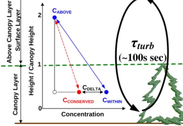
45 H e ig h t / C a n o p y H e ig h t S u rf a c e L a y e r C a n o p y L a y e r

τ

(~100s sec)

Figure 8.Schematic of our two-layered model based on the localized-near field, LNF, concept. 3

CABOVE represents the reference concentration, which for the above-canopy layer is defined as

4

the measured concentration at height 18m. CWITHIN is the measured concentration within the

5

canopy defined as the averaged concentration at 0.5, 5, and 9m. CCONSERVED is the estimated

6

concentration based on the measured eddy-covariance flux and the eddy diffusivity calculated 7

from sensible heat flux. CDELTA is the difference between CWITHIN and CCONSERVED and is a

8

measure of the importance of non-conservative processes. 9

10

Figure 8. Schematic of our two-layered model based on the

lo-calized near field, LNF, concept. CABOVErepresents the reference concentration, which for the above-canopy layer is defined as the measured concentration at a height of 18 m. CWITHINis the mea-sured concentration within the canopy, defined as the averaged con-centration at 0.5, 5, and 9 m. CCONSERVED is the estimated con-centration based on the measured eddy covariance flux and the eddy diffusivity calculated from sensible heat flux. CDELTAis the differ-ence between CWITHINand CCONSERVEDand is a measure of the importance of non-conservative processes.

when observations of fluxes are made above the roughness sublayer (Raupach and Legg, 1984) and this criterion was met at BEARPEX 2009 (18 m flux measurement height with 8.8 m mean tree height), as evidenced by a comparison of the flux data of the sensible heat and 3 biogenic VOC species, methanol, 2-methyl-3-butene-2-ol +isoprene, and monoter-pene, with longer chemical lifetimes than the turbulent trans-port time (Park et al., 2014).

The fluxes of reactive species cannot be completely de-scribed through simple application of similarity theory. This is because reactive species will, to some extent, undergo chemical transformations faster than they will be transported by turbulent diffusion (Vila-Guerau de Arellano et al., 1993; Gao et al., 1991; Jacob and Wofsy, 1990). However, similar-ity theory is still a powerful tool, as quantifying the flux due to turbulence transport allows for the estimation of the effects of other within-canopy chemical processes.

A visual representation of the idea proposed in this study is shown in Fig. 8. The red line shows the gradient ex-pected if flux–gradient similarity holds, and the blue line shows the gradient if the concentration is chemically, or otherwise, perturbed. This concept is known as localized near field (LNF) theory (Vandenhurk and Mcnaughton, 1995; Raupach, 1989). We apply LNF to conserved tracers and re-active molecules to test (1) whether the flux–gradient theory is valid within the canopy at this site and (2) whether the chemical reactivity or some other canopy processes affects the reactive chemicals. In the analysis below, we will assess the within-canopy behavior of H2O as conserved tracer and

NO, NO2, and NOxthrough pictorial relationships analogous

K.-E. Min et al.: Eddy covariance fluxes and vertical concentration gradient measurement 5505

In Fig. 8, the green dashed line divides two layers: a within-canopy layer and an above-canopy layer. CABOVEis

the measured concentration in the above-canopy layer and

CWITHIN is the measured concentration within the canopy.

Using similarity theory and the measured fluxes, we calcu-late CCONSERVED, the concentration that would be observed

for a conserved tracer. The difference between CWITHINand

CCONSERVED defines CDELTA, which represents the

contri-bution to the concentration by non-conservative processes that act to perturb the flux gradient relationship. To quan-tify CCONSERVED we use flux–gradient similarity, Eq. (2),

(Meyer, 1986) and the mixing rate, K, the so-called eddy diffusivity constant, which is inferred from the observed sen-sible heat flux and temperature gradient.

∂(CCONSERVED−CABOVE)

∂z =

Flux

K . (2)

In an illustrative test of our approach we present our results for the conserved tracer, water. In Fig. 9, the blue circles rep-resent the measured gradient of H2O and the red circles show

the gradient inferred from the H2O flux (CCONSERVED)in the

within-canopy layer at midday (from 12:00 to 14:00). The difference between CWITHINand CCONSERVEDin the

within-canopy layer, CDELTA, shown as a black arrow, is small (1 %

relative to CABOVE and within the concentration

measure-ment uncertainty of 3 %; the estimated propagated error is 15 % based on 10 % error in sensible heat flux calculation and 10 % error in K estimation). The small difference of

CDELTA,H2O is possibly due to the source/sink process

dif-ference with temperature and H2O. However, the magnitude

of CDELTA is smaller than the estimated uncertainty, so we

conclude that the sources/sink difference in H2O and

tem-perature are not detectable and the flux–gradient similarity holds for conserved tracer even within canopy at this site. This implies there is no measurable additional source/sink process(es) for H2O, aside from turbulent transport, and the

open canopy structure allows us to use flux–gradient simi-larity using within-canopy information. Similar results were obtained for CO2and several slowly reacting BVOCs (Park

et al., 2014).

Applying the same analysis to NO and NO2 (Fig. 10),

we find CDELTAis large compared to the measurement

vari-ability. CDELTA for NO is −12.4 ± 3.3 ppt (23 % relative to

CABOVE) and for NO2 is 64.7 ± 4.7 ppt (44 % relative to

CABOVE). We reach an identical conclusion, with slight

nu-merical differences, if we reference the calculation to the canopy top height instead of the average through the canopy, finding 27 and 39 % differences for NO and NO2compared

to the CABOVE, respectively. The estimated uncertainty in

the CDELTA calculation is 30 and 25 % (3.7 and 16.2 ppt)

for NO and NO2based on the error propagation. The paired ttest also shows statistically meaningful differences between

CWITHINand CCONSERVEDfor NO and NO2(p < 0.01).

Ex-amples of CDELTA analysis from individual days are shown

in Sect. S2 of the Supplement.

46 9.5 10 10.5 11 11.5 12 12.5 0 0.5 1 1.5 2 H 2O [ mmol/mol ] H e ig h t/ C a n o p y H e ig h t

C

Figure 9. The estimated concentration, CCONSERVED (red) using standard flux-gradient

3

similarities of H2O during midday (12:00-14:00) is shown. Blue represents the measured

4

vertical gradient. Open circles and whiskers represent the mean and the variability of H2O.

5

The difference between blue and red in the within-canopy level is shown in black arrow 6

indicates CDELTA and is negligibly small as expected for a conserved species.

7 8

Figure 9. The estimated concentration, CCONSERVED(red) using standard flux–gradient similarities of H₂O during midday (12:00– 14:00) is shown. Blue represents the measured vertical gradient. Open circles and whiskers represent the mean and the variability of H2O. The difference between blue and red in the within-canopy level is shown by the black arrow and indicates CDELTAand is neg-ligibly small, as expected for a conserved species.

Based on the observed gradient of NO, standard flux– gradient similarity predicts the downward flux of NO; how-ever, we observed an upward flux of NO (Fig. 7). This counter-gradient flux can only be explained by the formation of NO during the transport process from within the canopy layer to the above-canopy layer. Fig. 10a indicates that to ex-plain the observed NO flux, we need to account for 12 ppt

(CDELTA) more NO molecules than were observed in the

canopy layer. This is reasonable, as photolysis rates above the canopy should be faster than in the shade of the canopy. If the required NO were completely due to NO2photolysis it would

correspond to ∼ 12 ppt removal, or 20 % of the CDELTA of

NO2. The remaining 80 % of CDELTAin NO2, 52.3 ppt, must

be accounted for via other mechanisms.

To evaluate the contribution of photolysis of NO2 to the

counter-gradient flux of NO, we calculate the chemical con-version rate integrated over the 100 s (τturb)as Eq. (3).

PNO,net=LNO2,net=jNO2NO2 (3)

−(k_NO+O3[O3] +kNO+HO2[HO2] +kNO+RO2[RO2])[NO]

The photolysis rate, jNO2, is calculated with the Tropospheric Ultraviolet and Visible (TUV) radiation model scaled to the measured PAR. We treat RO2 as equal to HO2. Using the

measured concentrations of NO, NO2, O3, HO2, and

temper-ature, we estimate a net loss of 22.8 ppt (over 100 s) of NO2,

which is in excess of that needed to explain the NO counter-gradient flux of 12.4 (±3.3) ppt.

The large value of CDELTA for NOx(54.3 ± 5.9 ppt, 29 %

47 30 40 50 60 0 0.5 1 1.5 2 NO [ ppt ] C DELTA H e ig h t/ C a n o p y H e ig h t C a n o p y L a y e r S u rf a c e L a y e r 140 160 180 200 220 0 0.5 1 1.5 2 NO₂ [ ppt ] C DELTA Measured C_CONSERVED 1

Figure 10.The estimated concentration, CCONSERVED, (red) using standard flux-gradient

2

similarities of NO and NO2 at midday (12:00-14:00 and the measured vertical gradient (blue) 3

giving values for CDELTA of 12 ppt (NO) and 64 ppt (NO2). 4

5

Figure 10. The estimated concentration, C_CONSERVED, (red) us-ing standard flux–gradient similarities of NO and NO2at midday (12:00–14:00 and the measured vertical gradient (blue), giving val-ues for CDELTAof 12 ppt (NO) and 64 ppt (NO2).

within-canopy loss processes. To explore the mechanism(s) controlling the CDELTAfor NOx, we examine several

chemi-cal processes related to PNs, ANs, HNO3, and HONO using

our two-layer model (concept shown in Fig. 8). The mag-nitudes of each of the near-field processes for NOx were

inferred using Eq. (4) to estimate the contribution of cer-tain processes on the ∼ 100 s timescale of turbulent mixing (τturb). LXor PX= ∂ ∂t z2 Z z1 CX(z)dz (4)

Here, LX (PX) is the loss (production) rate of species X

happening within the time window of turbulent air move-ment from within the canopy (height z1)to above the canopy

(height z2). We chose 4.4 m, the middle level of the canopy,

as a representative of z1, and 18 m above-canopy layer as

representative of z2.

PNs can act as either a net source or a sink of NOxthrough

thermal dissociation (+1 NO2 molecule) or PN formation

(−1 NO2). Calculating the steady-state chemical

produc-tion and thermal and chemical loss of PAN (LaFranchi et al., 2009; Wolfe et al., 2009), yields 5.3 ppt of NO2formed

in 100 s. This mechanism implies an enhancement of NOx

within the canopy, as discussed in more detail in Min et al. (2014). However, we have also suggested that a local bio-genic precursor drives PN formation within canopy (Min et al., 2012). This BVOC PN species, denoted XPN, exhib-ited an upward flux and is a candidate for NO2 loss not

included in our steady-state calculation. We estimate the flux of this XPN to be 2.3 ± 0.4 ppt m s−1corresponding to 16.7 ppt of NO2loss within canopy and explaining 31 % of

the NOxCDELTA. 48 180 200 220 240 260 0 0.5 1 1.5 2 NO X [ ppt ]

C

DELTA

Figure 11. The estimated concentration, CCONSERVED, (red) using standard flux-gradient

2

similarities of NOX at midday (12:00-14:00) and the measured vertical gradient (blue) giving

3

values for CDELTA of 54 ppt (NOx). Open circles and whiskers are the mean and standard errors.

4

Figure 11. The estimated concentration, CCONSERVED, (red) using standard flux–gradient similarities of NOxat midday (12:00–14:00) and the measured vertical gradient (blue) giving values for CDELTA of 54 ppt (NOx). Open circles and whiskers are the mean and stan-dard errors.

BVOC-driven AN formation from OH initiated chemistry can be calculated as P_{P AN}=X i γiαikOH+VOCi[OH][VOCi], (5) where γi= kRO2i+NO[NO] kRO2i+NO[NO] + kRO2i+HO2[HO2] +PjkRO2i+RO2j[RO2]j+kisom . (6)

Here, αi and γi stands for the branching ratio of AN

forma-tion from RO2 and NO reaction, and the fraction of RO2i

from VOCi reacts with NO. Also, kisom refers to the

uni-molecular isomerization rate of RO2i. We estimate the effects

of MBO, monoterpenes and isoprene (important BVOCs at the BEARPEX site (Bouvier-Brown et al., 2009a; Schade et al., 2000) on AN production (for 100 s) and calculate that 3.1 ppt (5.7 %), 0.4 ppt (0.7 %) and 6.9 ppt (12.8 %) NOx is removed by AN formation, respectively. We use a

10, 11.7 and 18 % branching ratio (αi)for MBO (Chan et

al., 2009), isoprene (Paulot et al., 2009) and monoterpenes (Paulot et al., 2009). The rate constants and mechanisms for RO2+HO2, RO2+NO and RO2+RO2 were taken from

the Master Chemical Mechanism (MCM) v3.2 (Jenkin et al., 1997; Saunders et al., 2003) and isomerization rates for iso-prene from Crounse et al. (2011). If we consider AN forma-tion from ozonolysis reacforma-tions of very reactive BVOCs, such as sesquiterpenes in analogy to XPN formation through the channel described as BCSOZNO3 in MCM v3.2, we estimate an additional 16.8 ppt (31.1 %) of NOxconsumed over 100 s.

These calculations indicate chemical formation of nitrates is rapid enough to affect the fluxes.