Dynamic Application of Problem Solving Strategies:
Dependency-Based Flow Control
by
Ian Campbell Jacobi
B.S., Computer Science,
Rensselaer Polytechnic Institute (2008)
S.M., Computer Science and Engineering,
Massachusetts Institute of Technology (2010)
Submitted to the Department of Electrical Engineering and Computer
Science
in partial fulfillment of the requirements for the degree of
Engineer in Computer Science
at the
MASSACHUSETTS INSTITUTE OF TECHNOLOGY
September 2013
© Massachusetts Institute of Technology 2013. All rights reserved.
Author . . . .
Department of Electrical Engineering and Computer Science
August 30, 2013
Certified by. . . .
Gerald Jay Sussman
Panasonic Professor of Electrical Engineering
Thesis Supervisor
Accepted by . . . .
Professor Leslie A. Kolodziejski
Chair, Department Committee on Graduate Students
Dynamic Application of Problem Solving Strategies:
Dependency-Based Flow Control
by
Ian Campbell Jacobi
Submitted to the Department of Electrical Engineering and Computer Science on August 30, 2013, in partial fulfillment of the
requirements for the degree of Engineer in Computer Science
Abstract
While humans may solve problems by applying any one of a number of different prob-lem solving strategies, computerized probprob-lem solving is typically brittle, limited in the number of available strategies and ways of combining them to solve a problem. In this thesis, I present a method to flexibly select and combine problem solving strategies by using a constraint-propagation network, informed by higher-order knowledge about goals and what is known, to selectively control the activity of underlying problem solvers. Knowledge within each problem solver as well as the constraint-propagation network are represented as a network of explicit propositions, each described with respect to five interrelated axes of concrete and abstract knowledge about each propo-sition. Knowledge within each axis is supported by a set of dependencies that allow for both the adjustment of belief based on modifying supports for solutions and the production of justifications of that belief. I show that this method may be used to solve a variety of real-world problems and provide meaningful justifications for so-lutions to these problems, including decision-making based on numerical evaluation of risk and the evaluation of whether or not a document may be legally sent to a recipient in accordance with a policy controlling its dissemination.
Thesis Supervisor: Gerald Jay Sussman
Acknowledgments
I would like to acknowledge and thank the following individuals for their assistance throughout the development of the work presented in this thesis:
My advisor and thesis supervisor, Gerry Sussman, for his invaluable assistance and advice offered in the process of developing the ideas presented in this thesis.
Alexey Radul for developing the concept of propagator networks and assisting in troubleshooting and revising the propagator network implementation upon which the work in this thesis was based.
K. Krasnow Waterman for proofreading this paper and offering some interesting legal insights on several of the concepts presented in the thesis.
Lalana Kagal for her assistance and advice in developing reasoning systems, the lessons of which were integrated in part in the system proposed in this paper.
Sharon Paradesi for providing additional proofreading assistance and offering sug-gestions of several pieces of related work.
My lab-mates and other members of the Decentralized Information Group not named above for providing their assistance, criticisms, feedback, and proofreading skills on my presentations of this work as it has evolved over the past five years.
Finally, I would like to acknowledge that funding for this work was provided in part by Department of Homeland Security Grant award number N66001-12-C-0082 “Accountable Information Usage in Distributed Information Sharing Environments”; National Science Foundation Computer Systems Research/Software and Hardware Foundations Grant “Propagator-based Computing”, contract number CNS-1116294; National Science Foundation Cybertrust Grant “Theory and Practice of Accountable Systems”, contract number CNS-0831442; and a grant from Google, Inc.
Contents
1 Introduction 13
1.1 Defining Flexibility . . . 14
1.2 A Problem: Issuing Health Insurance . . . 17
1.3 A Solution (and Related Work) . . . 19
1.4 Thesis Overview . . . 22 2 Propagator Networks 23 2.1 Propagators . . . 23 2.2 Cells . . . 24 2.3 An Example . . . 26 2.4 Handling Contradictions . . . 29
2.5 Truth Maintenance Systems and Backtracking . . . 30
3 Five-Valued Propositions 33 3.1 Propositions . . . 33
3.2 Implementation . . . 35
3.3 Hypothetical Beliefs and Backtracking . . . 37
4 Building Problem-Solving Strategies 41 4.1 A Simple Rule . . . 41
4.2 Knowing the Unknown . . . 44
4.3 Making Work Contingent . . . 48
4.5 Controlling for Unknownness . . . 52
5 Building Justifications 55 5.1 What is a Justification? . . . 56
5.2 The Suppes Formalism . . . 57
5.3 Building Justifications . . . 59
5.4 Simplifying Justifications . . . 62
6 Propositions in Practice 65 6.1 The Problem . . . 65
6.2 Bootstrapping the System: Propositions . . . 66
6.3 Bootstrapping the System: Rules . . . 68
6.4 The System in Operation . . . 78
7 Beyond Propositions 85 7.1 Supporting Multiple Worldviews . . . 86
7.2 Proof by Contradiction . . . 88
7.3 Alternate Belief States . . . 88
7.4 Probability in Cells . . . 89
7.5 Contributions and Conclusions . . . 90
List of Figures
2-1 A propagator network which combines and converts the outputs of two
thermometers, converting between Fahrenheit and Celsius. . . 27
2-2 A propagator network merging the contents of cells. . . 28
3-1 The five values of a proposition . . . 36
4-1 A simple network of propositions connected by implication . . . 43
4-2 Code to prove ancestry through parenthood . . . 43
4-3 Code to prove ancestry through parenthood by way of a search . . . . 46
4-4 Code to prove ancestry transitively . . . 47
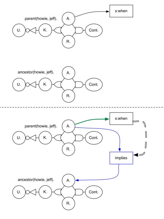
4-5 Lazily attaching a rule using teh s:when propagator . . . 49
4-6 Code to lazily prove ancestry through transitivity . . . 50
4-7 A simple syntax for lazily proving ancestry through transitivity . . . 50
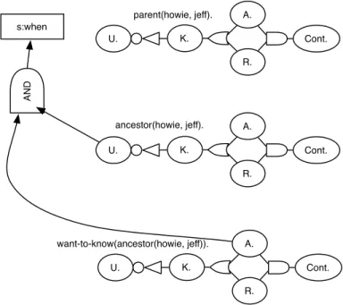
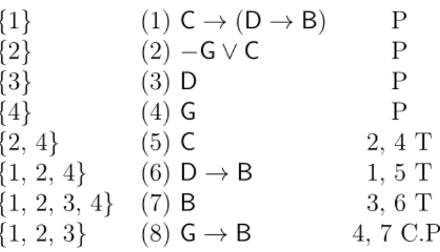
4-8 Controlling the search for ancestors only when such a search is needed 53 4-9 Code to control the search for ancestors only when a search is needed 54 5-1 A logical proof using Suppes’s formalism . . . 58
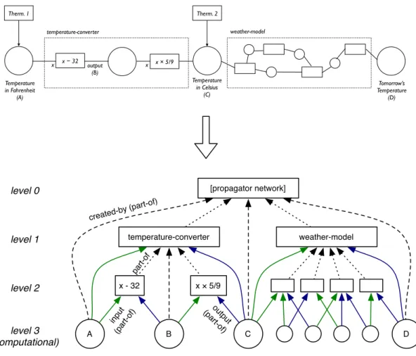
5-2 The semantic structure of a complex propagator network . . . 61
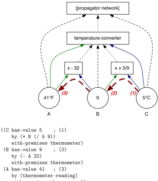
5-3 Recursive generation of a justification . . . 63
5-4 Generation of a simple justification . . . 64
6-1 Code for simplifications of thetell! function . . . 68
6-2 Asserted beliefs for Danny’s risk calculation . . . 69
6-3 Rules scoring insurance risk for sky-divers . . . 70
6-5 Conditioning the need to score risk from an unhealthy diet . . . 72
6-6 A propagator-based accumulator . . . 74
6-7 Adding a new input to a propagator-based accumulator . . . 76
6-8 Removing a contribution from a propagator-based accumulator . . . . 77
6-9 Code to accumulate value when there is such a need . . . 79
6-10 Code to accumulate risk only when there is a need . . . 80
6-11 A simple justification . . . 82
6-12 A more detailed justification for rejection . . . 83
List of Tables
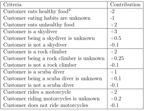
1.1 Contributions to risk score based on personal behaviors . . . 17
1.2 Rules for determining risk . . . 19
6.1 Contributions to risk score based on personal behaviors . . . 66
Chapter 1
Introduction
What differentiates human intelligence from that of other animals? Although sci-entists have proposed a number of different theories and differentiators in the past, including tool use [20], self-recognition [13], and social intelligence [10], each has been dismissed by later evidence of animals which exhibit behavior like that of humans. One of the leading theories at present is the human ability to solve problems in a abstract, “symbolic” manner [29]. Indeed, humans appear to use symbolic problem solving skills in any number of different ways, including the use of logic in statistical analysis based on the scientific method, as well as the application of probabilistic ap-proaches to learning which have formed the foundation of many algorithms considered to fall under the guise of “artificial intelligence” [25].
While the increased understanding of each of these problem solving mechanisms has led to a greater understanding and appreciation of the role of symbolic manipu-lation in human intelligence, less has been done to properly understand and harness the control of mechanisms that allow humans to make use of any of these approaches in a flexible manner, outside of work relating to Minsky’s theory of the Society of Mind [17, 18]. If we are to actually claim we understand the basis of human intel-ligence, we must also be able to discover the source of flexibility in human thought which allows us to effectively and efficiently solve problems using any number of prob-lem solving methods without any preconceived algorithms of how such control may be implemented.
1.1
Defining Flexibility
If we are to discuss flexibility of human problem solving skills, we must better define what exactly is meant by this term. Human problem solving appears to feature a number of aspects which, while perhaps not entirely unique to humans, are features which we see as integral to the ability to solve problems. Some of these attributes include reactivity, goal-oriented behavior, synthesis of disparate attributes (such as color and location), apparent optimizations for certain kinds of problems, resilience to contradictory inputs, and the ability to evaluate and select from different strategies using what appears to be a single mechanism of thought.
While reactive behavior is common to practically all living things (e.g. subcon-scious reflexes), humans appear uniquely able to react not only to physical constraints which manifest while solving a problem, but also to theoretical, symbolic constraints, such as those presented in hypothetical situations and those which occur in abstract conceptual reasoning (e.g. making reactive decisions about perceived social and finan-cial situations). Indeed, the ability to combine, apply, and otherwise utilize abstract, symbolic values and operations is viewed as such a fundamental component of human thought that its development in the adolescent human psyche is viewed as a transition between the final two developmental stages in the theory of cognitive development proposed by Jean Piaget (concrete operational and formal operational) [4].
Such reactivity is particularly evident in humanity’s ability to engage in long-term planning. Indeed, humans appear to be the only species capable of planning beyond their lifetime and those of their heirs. When knowledge about specifics will necessarily change over time, there is a need to adjust any strategies seeking extremely long-term results to account for large-scale changes in the environment. Human attempts to address or account for issues such as global warming, technological development, and large-scale societal change are but some examples of such behavior. Although humans often encounter practical difficulties in envisioning and planning on extremely long time-frames, such limitations appear to be cultural in nature (e.g. a drive for short-term profits), rather than inherent to human intelligence. Indeed, some social groups
have proven quite willing to solve problems on time-scales beyond many hundreds of years [1].
Human problem-solving is not only reactive, it is also goal-oriented. On the most basic level, the desire to solve a problem implies that there is a fundamental goal: the solution of the problem. But goal-direction may also be observed in the ability of humans to plan how such problems will be solved, typically by establishing sub-goals which may be achieved on the way to solving the larger problem. Such management of sub-goals appears to act at even a sub-conscious, fundamental level in human thought; a neuroimaging study by Braver and Bongiolatti [2] has implicated the frontopolar region of the prefrontal cortex of the human brain in managing subgoals associated with primary goals in working memory tasks.
The ability to synthesize disparate data appears to be another unique feature of symbolic thought. Research by Herver-Vazquez, et al has shown that humans are capable of synthesizing information about geometric features and landmarks to identify locations [9], an ability not observed in rats. Thus, if a problem solving mechanism is to approach human capabilities, it must be able to synthesize arbitrary features to derive solutions, lest such a mechanism be unable to solve the deceptively simple task of locating an object using both geometric and landmark-based cues, such as locating the Washington Monument in Washington, D.C. based on the fact that it is “at the opposite end of the Reflecting Pool from the Lincoln Memorial.”
It is often argued that humans are “efficient” thinkers. Although this is rarely well-supported in practice, as humans easily fall prey to the inefficiencies of classi-cal NP-hard problems, there are indications that humans are uniquely positioned to solve certain kinds of problems. Indeed, recent studies making use of functional mag-netic resonance imaging and transcranial magmag-netic stimulation have begun to identify different regions of the brain which appear to be relevant for social and emotional reasoning [33, 30] as well as “creative” thought such as analogy and metaphor [26, 32]. It is similarly likely that a general-purpose, flexible problem solver must be able to select from efficient, smaller problem solving components which are specialized at solving parts of a larger problem.
Human intelligence is also notable for its ability to handle contradictory beliefs, contrary to the tenets of classical logic, which necessarily imply that simultaneous belief in two contradictory statements necessarily renders all statements true (i.e. ex falso quodlibet ). This suggests that human thought may not be founded in the realm of classical logic. Instead, humans may be capable of thinking within a superset of such logic.1
The flaws of classical logic with respect to non-contradiction are hardly universal however, and other logics may yet prove to be the basis of thought. Modern logics, such as Belnap’s four-valued logic [14], that take into account paraconsistency, in which contradictions should not cause an “explosion” of conclusions, or logics that adhere to dialetheism, in which contradictions may exist as facts, seem to embody much more pragmatic modalities for man’s rational thought. The rational thinker attempts to resolve observed contradictions by revising his beliefs, not by breaking down.
Most important, however, is humanity’s ability to apply a wide variety of different approaches to solving the same problem. For example, the Pythagorean theorem may be demonstrated by way of any one of dozens of methods, including algebraic solutions, geometric rearrangement, and even proofs based on dynamic systems (i.e.
physics) [15]. While the symbolic thought of a single human does appear to be
constrained to follow a single approach at any given time (i.e. humans have a difficult time thinking about multiple unrelated ideas at the same time), not only are humans free to apply different approaches based on personal judgments made while solving a problem, but humans may even derive and learn new approaches to solve novel problems which have yet to be encountered. These approaches may then be applied in the future. Any system that attempts to achieve a modicum of intelligence must be prepared to be flexible in its approaches to problem solving in these ways, or it is unlikely that it will truly resemble the abilities that may be achieved by a human.
1The mere existence of human logicians suffices as demonstrative proof that classical logic may
Criteria Contribution
Customer eats healthy food2 -2
Customer eating habits are unknown -1
Customer eats unhealthy food +2
Customer is a skydiver +3
Customer being a skydiver is unknown +0.5
Customer is not a skydiver -0.1
Customer is a rock climber +2
Customer being a rock climber is unknown +0.25
Customer is not a rock climber -0.1
Customer is a scuba diver +1
Customer being a scuba diver is unknown +0.1
Customer is not a scuba diver -0.1
Customer rides a motorcycle +2
Customer riding motorcycles is unknown +0.2
Customer does not ride motorcycles -0.1
Table 1.1: Contributions to risk score based on personal behaviors
1.2
A Problem: Issuing Health Insurance
As an example of the flexibility of humans in solving problems, consider the following scenario:
Sally is an insurance underwriter working for Aintno, a health insurance company. As the entirety of the reforms of the Patient Protection and Affordable Care Act have not yet been put into place as of 2013, it is still possible to reject applications for individual health insurance policies. Sally’s job is to review the files of prospective customers to determine whether or not they should be issued insurance.
When issuing insurance, Sally must determine Danny’s eligibility in accordance with Aintno’s eligibility policies, which determine such based on a system which scores the risk of insuring a prospective customer based on a number of different criteria. For each criterion that an individual meets, their risk score is adjusted appropriately (See Table 1.1). Once a final score has been calculated, it is compared with several thresholds. If the risk score is less than the minimum risk score threshold of 2, Aintno will issue an insurance policy to the customer. However, if the risk score is greater than the maximum risk score threshold of 3, Aintno will refuse to issue insurance to
the customer. If the risk score is between 2 and 3, Aintno will attempt to do more work to determine whether insurance should be issued.
When Sally arrives at her desk one morning, she finds that she has been given the file of Danny, a young adult looking for health insurance. As a prospective customer, Danny’s eligibility must be determined before insurance may be issued. If he is not eligible, then Sally must note that insurance was denied, and, so as to be able to defend such denial in legal proceedings, must note the reasons which lead to the denial (i.e. the facts which led to the excessively high risk score).
Similarly, if he is eligible, she must finalize an offer to insure Danny. In this case, she must still note the risk score and the sources of the risk, as the sources and amount of risk are relevant to determine what Danny’s insurance premiums should be.
In order to determine Danny’s risk score, she starts up Aintno’s custom risk anal-ysis program and begins to input the data from Danny’s file, including his Facebook
and Flickr social network profiles3, which were gleaned from an optional field which
had been filled in in Danny’s file. As she does, Aintno’s risk analysis program mines the two profiles for useful information which may be used to determine Danny’s risk. Initially, the program attempts to score Danny’s risk on the basis of criteria other than his diet, as Aintno’s policy is to avoid making such determinations if at all possible due to the perceived subjectivity and fluidity of customers’ diets. It identifies Danny as high-risk, however, due to his engaging in motorcycling and skydiving. Together with his inability to prove he is not a rock climber and his lack of SCUBA diving experience, Danny has a total risk score of 5.15.
Sally prepares to issue a denial to Danny, but then remembers that, due to a law recently passed in Danny’s home state, Aintno is not permitted to mine Facebook for insurance purposes. She directs the program to remove all facts that depended on Facebook. This drops his risk score to 2.15 (as the fact that he engages in skydiving 3Although the use of information from social networks has not been used in underwriting as in
this example, some insurers already use information from social networking sites in fraud cases [22], and a recent study by Deloitte Consulting and British insurer Aviva PLC found that a predictive model based on consumer-marketing data such as hobbies and TV-viewing habits was judged as largely successful in comparison with traditional underwriting, finding that “the use of third-party data was persuasive across the board in all cases” [27].
eats(subject , food ) ∧ unhealthy(food ) → eats(subject , unhealthy-food)
likes(subject , thing) ∧ is-a(thing, food) → eats(subject , thing)
likes(subject , place) ∧ is-a(place, restaurant) → eats-at(subject , restaurant )
works-at(subject , place) ∧ is-a(place, restaurant) → eats-at(subject , restaurant )
(eats-at(subject , place) ∧ is-a(place, restaurant) ∧ primarily-serves(place, thing)
∧ is-a(thing, food)) → eats(subject , thing)
Table 1.2: Rules for determining risk
was only found on his Facebook profile), and causes the system to do more work and activate a set of rules regarding Danny’s eating habits.
As Danny works at Hal’s Hot Dogs (a hot dog restaurant), a number of pre-programmed rules which assist in assessing and accumulating risk scores based on eating habits (See Table 1.2) determine that Danny is a likely consumer of hot dogs, an unhealthy food. As a result, Danny’s risk score is returned to an unacceptably high 4.05. Thus confident in Danny’s ineligibility, she finalizes the rejection of Danny’s policy.
1.3
A Solution (and Related Work)
Certainly individual components of this problem could be solved using existing rule systems, data mining tools and a simple score aggregation algorithm. But what would it take to remove Sally from the equation altogether? Could we automate the process of determining eligibility and eliminate the role of the human altogether?
A naïve approach to such automation would simply result in a domain-specific so-lution by determining the requirements and rules surrounding Sally’s workflow. From a low-level perspective, we may consider the act of receiving a request for analysis to drive the process of reading and interpreting Danny’s file, which subsequently causes work to be done to mine and analyze information connected through his Facebook and Flickr profiles, not only to better inform about lifestyle choices Danny may not have been asked about in his application, but also to determine whether Danny’s application may contain missing or incorrect information.
Evidently, then, automation is possible, but we are left with two subtle issues in accepting this naïve approach to problem solving:
1. Such a domain-specific solution is likely to be brittle and require careful re-tooling as rules, regulations, and inputs change. For example, if Flickr increases the cost (be it computational or financial) of accessing the data it provides, the heuristics used to guide the analysis are likely to change. Rather than querying Flickr for every application, Aintno might only wish to query Flickr for additional details if other parts of Danny’s application suggests that he might be lying on his application, but proof is lacking. How can we make this solution flexible depending on changing inputs and rules?
2. While we have a method of producing a domain-specific solution correspond-ing to a workflow to solve a particular problem, this still doesn’t address the fundamental act of problem solving in and of itself. It captures nothing of the flexible planning and thought which we associate with true intelligence, as work is likely forced into a procedural rather than declarative mode. Is it possible to generalize this problem-solving approach so that we rely on domain-specific input knowledge rather than a domain-specific problem solver?
In short, such a domain-specific solution does not capture the true nature of human intelligence. Much of the flexibility and power of the human mind is left behind during the process of building the solution according to the constraints of the problem. The fact that a human may calculate this risk in a number of innovative ways is lost when an automated solution is constructed, as such automation ultimately implements only one such method. As a result, naïve, brittle problem-solving mechanisms cannot be reused and may find difficulty in integrating with other domains.
Instead, I propose a system in which knowledge is expressed in terms of orthogonal axes of beliefs. These beliefs may be connected in such a way that control may be made explicit through the expression of appropriate beliefs (e.g. a “need to support” some belief may drive work to uncover proof which supports that belief). These
connections also allow these beliefs to propagate through a network of operators which effect work so as to meet goals expressed as other beliefs.
In some respects, this interlinkage between goals, knowledge, and actions resembles Marvin Minsky’s K-line theory [16], in which relevant knowledge, stored and orga-nized hierarchically, may be used to configure perceptive units (P-agents) to create partial “hallucinations” of perception to assist in achieving goals and solving prob-lems. By synthesizing “missing” perceptions, Minsky argues that existing problems are more readily aligned with previously encountered ones, allowing for the selection of the mechanisms best suited to solving them.
Relevant to the work presented here is Minsky’s extension of the K-line theory to include an additional “G-net” of goals which influence which knowledge is likely to be relevant at a given time. Just as knowledge may influence perception through the activation of K-lines, Minsky proposes that goals may influence the activity and application of knowledge (and thus, indirectly, perception) through the connections that exist within the net of goals as well as perceptions.
The problem solving strategy proposed here resembles K-line theory, and treats goals, knowledge, and perceptions as independent beliefs which may be connected by a network of computational propagators which propagate beliefs between various statements of goals, knowledge, and perceptions. In this way, a goal which is estab-lished to calculate Danny’s risk may establish a belief in another goal which expresses a “need to know” what Danny’s eating habits are. This system also provides a mech-anism for connecting these goals, knowledge, and perceptions to systems which do practical work (e.g. reasoning, discovery mechanisms, or aggregation of values), and as such moves beyond K-line theory to demonstrate the practicality of such a theory. It is worth noting that the system presented in this thesis also owes a significant debt to the work done by de Kleer, et al on the AMORD system [5]. In addition to making use of truth maintenance systems to maintain dependencies and enable backtracking in reasoning, the propositional model also allows for the expression of rules and the assumption and retraction of various premises made possible by TMSs as a whole, a concept inspired by the work done in AMORD to do likewise.
Unlike AMORD, however, the “belief propagation” system presents an alternative, more general view of belief. Where AMORD implicitly assumes that a belief is a positive “assertion” of truth, this thesis takes the position that a particular “fact” or proposition may have a number of different beliefs associated with it, including acceptance of the proposition (i.e. the affirmative belief that the proposition is true), rejection of the proposition (i.e. the negative belief that the proposition is false), as well as simple beliefs which express the presence or absence of knowledge regarding the proposition entirely. As a result, the propositional system proposed here permits a greater amount of control than AMORD does, due to the greater expressivity of the propositional system.
1.4
Thesis Overview
This thesis seeks to outline the belief-propagation mechanism proposed above, which achieves such flexibility in problem solving by modeling knowledge with respect to support for a given belief. These models are built on top of the propagator net-work model, described in Chapter 2, and the proposition model of knowledge is then proposed in Chapter 3. Chapter 4 then illustrates how the propositional knowledge model may be used to solve problems in a flexible manner. Chapter 5 explains how the belief propagation mechanism may be used to construct meaningful explanations for the results of such problem solving. Finally, Chapter 6 demonstrates an example of the propositional knowledge model while Chapter 7 offers some directions for future work.
Chapter 2
Propagator Networks
The flexible problem solving mechanism described in this thesis depends on the pow-erful computational substrate called propagator networks, developed by Alexey Radul and Gerald Jay Sussman [21]. This computational substrate provides a simple mech-anism for maintaining and updating partial information structures so that partial information about an attribute or value may be refined over time. In this chapter, a short description of the technology is provided in this chapter so that the reader may better understand the mechanism of the propositional system explained in subsequent chapters.
2.1
Propagators
Propagator networks consist of a network of two kinds of elements. Propagators are small computational units which do work on various inputs stored in single-storage memories known as cells. Any propagator may do work based on data in zero, one, or more cells, and may store output in one or more output cells. This work may range from simple operations such as addition and subtraction to complex calculations and algorithms. In principle, most complex operations are performed by networks of simple propagators representing basic mathematical operators and “switches” in the propagator network, which alternately connect one of several input cells to an output cell.
Propagators serve much the same purpose as electronic components do in an electrical circuit; the ways in which simple propagators are connected help to define the contents of cells at any given point, much as electronic components will influence the voltage and current at any given point in a circuit.
Propagators also resemble electronic components in another way: just as partial circuit diagrams may be abstracted and reused as “compound circuits” (such as with integrated circuits), partial propagator networks may be abstracted and reused as “compound propagators”. As these compound propagators become active, they con-struct the partial propagator network represented by the compound propagator, thus permitting for recursion and the constrution of loops.
For example, a “factorial” propagator might expand into a network consisting of a subtraction propagator to subtract 1 from the input, another factorial propagator to calculate the factorial of one minus the input, a switch to determine whether that factorial should become active (e.g. if the input is less than 1), and a multiplication propagator which multiplies the output of the “inner” factorial propagator with the input of the “outer” factorial propagator. Then, if the input is much greater than one, the inner factorial propagator will be activated to calculate the factorial recursively.
2.2
Cells
The other component of a propagator network, the cell, acts as the glue of the prop-agator network; it stores data which may be used by propprop-agators to do computation. The information stored in a cell may be updated at any time by a propagator which sends an “update message” to that cell. This message contains any new information which may be used to inform the contents of that cell by merging the contents of that message with the data currently in the cell using an appropriate merge operation.
The merge operation used to combine the update message and the existing infor-mation in a cell is selected based on the type of data stored in the cell and the type of data provided in the update message. For example, if a cell stores a numeric interval and receives another numeric interval in an update message, it may merge the update
by taking the intersection of the two intervals. In this way, the information stored in the cell may be gradually refined by obtaining ever narrower estimated ranges of the value of the cell.
When a propagator network is constructed, propagators may be registered as neighbors of cells so that they may be alerted when the cell’s content changes. Once a cell has finished merging its content with the content in the update message, those neighboring propagators will be alerted and given an opportunity to do additional work, typically by making use of the newly updated value of the cell. These alerted propagators may then send updates to other cells. As a result, updates to the content of a cell will effectively propagate across the network of propagators and cells.
As the numeric range example demonstrates, the ability to use merge operations to gradually refine the information stored in cells means that propagator networks readily lend themselves to the representation and manipulation of partial information. Rather than representing complete knowledge about a value, the concept of partial information means that, while the attribute or variable which is represented by the partial information is fixed, the value of the attribute itself may be incomplete, and extended as more information is known.
For example, in the numeric range example above, a cell might represent the outside air temperature, even though the actual value of the cell is a range with lower and upper bounds. In this sense, the inherent errors in measurement may be made explicit, so that, rather than some complete, presumably unmeasurable, value, we give a range that the actual temperature lies within. That is, by providing lower and upper bounds on the temperature, we are giving partial information about the temperature, rather than full information.
Cells which store partial information may, with appropriate merge operations, build up the partial knowledge in a cell when an update is received, so as to ob-tain a better, more informed, value. In the numerical range example above, range intersection is an appropriate merge operation, as it may be used to refine multiple, potentially equally broad, ranges to obtain a more precise answer than any one of the “input ranges” on their own.
2.3
An Example
Consider a system which seeks to measure the local air temperature in Boston in degrees Celsius using two thermometers. Like any practical measurement device, these thermometers have an error range and are not guaranteed to measure the actual temperature. These thermometers do not behave identically, so they may report different temperature ranges. Given this fact, it is possible to obtain a more accurate measurement of the temperature by considering the intersection of their error ranges. In addition to their measurement flaw, these thermometers have one other practi-cal flaw, in that they measure the temperature using different spracti-cales. One measures the temperature in degrees Celsius, while the other measures in degrees Fahrenheit. As a result, care must be taken to ensure that the measurements of the thermometer which reads in Fahrenheit are converted to degrees Celsius.
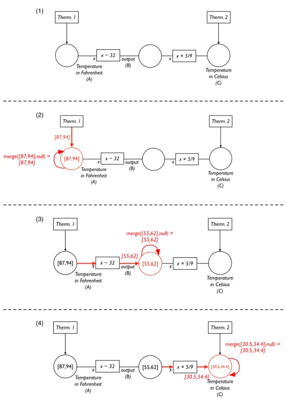
Given this fact, we may consider solving for the temperature of the thermometers in degrees Celsius using a simple propagator network, given in Figure 2-1-1. Here, the thermometers act as propagators which update cells with their estimate of the temperature range. When the Fahrenheit thermometer reports its temperature (as in Figure 2-1-2), it sends an update to the Fahrenheit temperature cell, cell A. This cell is then connected to a subtraction propagator, which will subtract 32 from the contents of cell A and update the value in the output cell (B) with the newly calculated intermediate value of the conversion (Figure 2-1-3). A second propagator is connected
to that intermediate cell B and will multiply that value by 59, and use that value to
update the Celsius temperature in cell C (Figure 2-1-4).
Note that in all steps in Figure 2-1, the cells to which updates are sent simply adopt the contents of the update message to be their new content. This is due to the fact that the cells initially contain a null-like value, “nothing”. This null-like value is the initial value of a cell, and represents a lack of any partial information about the cell’s value whatsoever. Thus, since there is no partial information with which the numeric range in the update data can be merged, the merge operation simply sets the value of the cell with the initial, “more specific” partial value given in the update.
(1) (2) (3) (4) Temperature in Fahrenheit (A) Temperature in Celsius (C) x − 32 x output (B) x × 5/9 x Therm. 1 Therm. 2 [87,94] Temperature in Fahrenheit (A) Temperature in Celsius (C) x − 32 x output (B) x × 5/9 x Therm. 1 Therm. 2 [87,94] [55,62] [87,94] Temperature in Fahrenheit (A) Temperature in Celsius (C) x − 32 x output (B) x × 5/9 x Therm. 1 Therm. 2 [30.5,34.4] [55,62] [87,94] Temperature in Fahrenheit (A) Temperature in Celsius (C) x − 32 x output (B) x × 5/9 x Therm. 1 Therm. 2 merge([87,94],null) = [87,94] merge([55,62],null) = [55,62] [55,62] merge([30.5,34.4],null) = [30.5,34.4] [30.5,34.4]
Figure 2-1: A propagator network which combines and converts the outputs of two
thermometers, converting between Fahrenheit and Celsius. A temperature range
from thermometer 1, in degrees Fahrenheit, (2) is sent to a cell. This alerts a chain of propagators responsible for converting the temperature range to Celsius (3, 4).
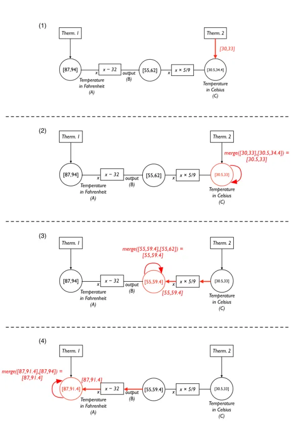
(1) (2) (3) (4) [30.5,33] [55,59.4] [87,94] Temperature in Fahrenheit (A) Temperature in Celsius (C) x − 32 x output (B) x × 5/9 x Therm. 1 Therm. 2 [30.5,33] [55,59.4] [87,91.4] Temperature in Fahrenheit (A) Temperature in Celsius (C) x − 32 x output (B) x × 5/9 x Therm. 1 Therm. 2 [30.5,34.4] [55,62] [87,94] Temperature in Fahrenheit (A) Temperature in Celsius (C) x − 32 x output (B) x × 5/9 x Therm. 1 Therm. 2 [30,33] [30.5,33] [55,62] [87,94] Temperature in Fahrenheit (A) Temperature in Celsius (C) x − 32 x output (B) x × 5/9 x Therm. 1 Therm. 2 merge([30,33],[30.5,34.4]) = [30.5,33] merge([55,59.4],[55,62]) = [55,59.4] merge([87,91.4],[87,94]) = [87,91.4] [87,91.4] [55,59.4]
Figure 2-2: Propagator networks merge the existing contents of cells with updates received from propagators. An update in degrees Celsius from thermometer 2 (1) is merged with existing knowledge of the temperature (2) and propagates to the output cell containing the temperature in degrees Fahrenheit (3, 4).
However, when the second thermometer sends its temperature reading in degrees Celsius as an update to cell C (Figure 2-2-1), the cell actually takes the intersection of the current value in cell C and the value in the update and uses that value as the new value of the cell (Figure 2-2-2). Propagators may, of course, be constructed as reversible operations so that an update of an “output” may refine the “input”. In Figures 2-2-3 and 2-2-4, the multiplication and subtraction propagators act reversibly and and divide and add to update the temperature range in degrees Fahrenheit in cell A. As a result, the Fahrenheit temperature range in cell A is also an intersection of the two ranges.
2.4
Handling Contradictions
While Figure 2-2 demonstrates the value of refining numerical ranges by taking their intersection, this raises a conundrum: what if the range in the update does not intersect the range currently stored in the cell? Or more generally, what if an update to a cell contains information which contradicts what is already stored in it?
When humans encounter a contradiction in practice, they typically desire to re-solve the contradiction to obtain a new, reliable value from which additional work may be derived. Such resolution may be done in many ways, and often results in additional work being done to determine a resolved value. For example, if a tempera-ture range contradicts an existing estimate, it may be appropriate to “kick out” older contributions which may not accurately represent the current value of a changing tem-perature. It might also be appropriate to determine whether a given thermometer is broken or unusually inaccurate. If so, this may prompt a user to repair or remove the faulty thermometer.
Because the ways in which a contradiction may be resolved may vary drastically depending on the contents of the cell and the nature of a problem to be solved by the network, implementations of propagator networks should be flexible in handling any conflicts. The implementation of propagator networks in the MIT/Scheme program-ming language, which has been used as the basis for the work in the remainder of
this thesis, normally raises an exception when a contradiction is encountered, causing computation to halt so that humans may examine the nature of the contradiction and resolve it in an appropriate manner.
Requiring human intervention is not a practical solution for most problems, how-ever; it would be untenable to require human input to abort every “dead-end” in a computation by removing inappropriate inputs, especially in the large search spaces that lie at the core of many kinds of problems. While the underlying propagator network mechanism may not directly support contradiction handling, the flexibility of the “cell merge” operation permits basic contradiction handling to be performed as part of the logic of such merge operations. The data structure known as a truth main-tenance system, or TMS, has several features which make it particularly appropriate for handling contradiction resolution in their merge operation.
2.5
Truth Maintenance Systems and Backtracking
Truth maintenance systems (TMSs) [6, 7] are data structures which allow for the maintenance of a variable’s value based on the set of minimal supports or premises for a given value. Although there are several kinds of truth maintenance systems, assumption-based truth maintenance systems (ATMSs) are among the most useful to track all possible premise-set/value pairs known to be valid for a given variable. They may also be “queried” to retrieve the value that is best supported by a given set of premises. Such values may be returned with the minimal set of premises known to support the value, conveniently allowing for the identification of the subset of premises most relevant to the specification of the returned value.
TMSs1 are appropriate contents for cells, as they may be merged by simply taking
the union of the set of value-support pairs in a cell and a set of such pairs in the update message. The union of the sets of value-support pairs may then be treated and stored 1It is worth noting that not all of the powers I have mentioned in this section are available in
other kinds of truth maintenance systems (such as justification-based truth maintenance systems or logical-based truth maintenance systems). As a result, whenever I mention truth maintenance systems (TMSs) hereafter in this thesis, I refer to assumption-based truth maintenance systems.
as the new contents of the cell, so that smaller support sets for an otherwise identical value may be propagated through neighboring propagators to their output cells.
By storing values as a function of a set of premises, TMSs may mark these sets as “no-good” when contradictions are identified during the merge process (i.e. when two value-support pairs with different values are supported by the set of premises) and resolved through manipulation of the premise set at merge-time. Such premise-set manipulation may change the effective value of a cell without actually introducing a contradiction in the actual value stored in the cell; the contents of the TMS grow and change independently from the set of believed premises, which are not subject to the contradiction behavior of the underlying propagator network itself.
Manipulation of the premises during the cell merge operation introduces the abil-ity to implement algorithms which require a backtracking search. When a particular premise propagates to a cell and creates a contradiction in a TMS value when the merge operation is applied, the TMS merge operation may effectively retract that premise so that other premises may be tested for a suitable solution. In short, search-ing for the solution to a problem ussearch-ing propagators becomes simply a matter of searching for the set of premises which solves a problem without causing any contra-dictions.
But while backtracking is but a necessary technique for problem solving, it is not the whole story. Propagator networks and truth maintenance systems provide a powerful mechanism which may be used to solve problems, they are still nothing more than a computational platform, and they lack any features which might assist in higher-order problem solving strategies. To actually attack problems and control problem solving based on needs, desires, or beliefs, we need a way to represent these needs, desires, and beliefs beyond the simplistic value maintenance of a TMS. For that, we must turn to the idea of the proposition.
Chapter 3
Five-Valued Propositions
Controlling problem solving systems requires representations of both those beliefs that act as input to the problem solvers and those beliefs which may be used to control the problem solving itself. While the facts about Danny’s hobbies may be sufficient to determine that he should not be granted insurance coverage, in practice, it is necessary to be able to express and recognized the need for this determination before it may happen. I have represented both the these needs and facts used as input for problem solving in the form of propositions.
3.1
Propositions
A proposition is any statement which may be believed to be true or false. Propositions differ from traditional logical statements in so far as they have no inherent truth or falsehood in and of themselves. The existence of a proposition does not imply that the proposition is true; propositions represent merely the concept of a statement without any associated belief. To represent the nature of belief in a particular proposition, each proposition is considered in terms of five different axes of belief: acceptance, rejection, contradiction, knowledge, and ignorance.
The first two axes, acceptance and rejection, correspond to belief in the truth and falsehood of the proposition, respectively. That is, a proposition is accepted if it is believed to be true, while a proposition is rejected if it is believed false. Note
that truth and falsehood are independent of one another! It is quite possible for a proposition to be both accepted and rejected (albeit temporarily), or to be neither accepted nor rejected. By separating these two concepts as two distinct axes of belief facilitates the expression of complex combinations of the support for and against a particular proposition which may be evaluated differently in different contexts.
The remaining beliefs may be expressed in reference to acceptance and rejection. Acceptance and rejection may be considered together to determine whether there is a contradiction in beliefs. Such a contradiction may force problem solvers to backtrack by removing certain assumptions that may have led to such contradictory beliefs.
Where the contradictory state of belief is the conjunction of acceptedness and rejectedness, knowledge (or knownness) is the disjunction of acceptance and rejection. A proposition is known if there is support for the proposition to be either accepted or rejected. Similarly, a proposition may be unknown entirely (i.e. the system may be ignorant of any knowledge regarding the proposition) if there is no support for it being either accepted or rejected.
This alternate metric of ignorance is what provides for flexibility and control in problem solving; it is possible to use a lack of knownness to determine when work should be done to determine a solution. Often, once a proposition is believed to be true or false, it is unnecessary to expend additional effort to uncover additional support. For example, in the Aintno example, there is no need to calculate a com-plete risk score for insurance purposes; once sufficient evidence has been gathered to determine that insurance should be denied, the work performed to acquire additional evidence for denial is unnecessary, as the relevant determination (whether the claim should be accepted or rejected) is already made. (But this does not mean that work cannot be done later if the evidence changes!)
What is important for all of these facets of knowledge and belief is that each state of belief is only loosely connected to the others. Excepting the basic logical
relationships (e.g. simultaneous acceptance and rejection is contradictory, and a
proposition cannot be both known and unknown), support for each belief state is independent and can be used to drive problem solving separately from belief in any
of the other belief states. As a result, each belief state may drive problem solving in a different manner appropriate to the problem. If the problem requires it, ignorance may be used to control when work is done to prove acceptance or rejection, but this is not a requirement. Similarly, the belief in the rejection of a given proposition may be used to drive computation to disprove such rejection (e.g. if there is a strong desire to prove acceptance through contradiction).
3.2
Implementation
The evaluation of a proposition with respect to five values is an important foundation of expressing belief, but how are we to actually represent this knowledge and its connections to other beliefs? If we are to properly link propositions so that their beliefs influence each other and so that computation and problem solving is contingent on the nature of belief, we may wish to construct a network of propositions using propagator networks, so that different states of belief in a proposition are able to influence and modulate beliefs in other propositions. In this way we may cause computation to occur.
This use of the propagator architecture for “belief propagation” bears many sim-ilarities to constraint propagation systems, first described by David Waltz [31]. In particular, the relationships between beliefs which are expressed with respect to state-ments may be considered edges which constrain the beliefs on either end of the rela-tionship. For example, a rule A → B may be represented by a connection between an affirmative belief in A and an affirmative belief in B, as well as a second connection between a negative belief in B and a negative belief in A.
While combining constraint propagation and logical programs is admittedly not a novel idea [12], the propositional architecture exposes program control structures and integrates them into the system of constraints. Rather than simply delegating and expressing logical relationships as constraints themselves, this architecture allows for the amount of work done to “prove” a logical statement to itself be constrained on the basis of belief in other statements.
∧
∨
~
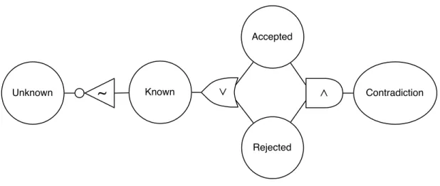
Contradiction Unknown Known Rejected AcceptedFigure 3-1: A proposition may be described with respect to five values connected in a propagator network of logical operations. Each circle represents a “cell” containing the data in support (or opposition) of that particular belief state, and the currently supported value will propagate its dependencies to related belief states as needed based on the nature of belief.
For example, it should be possible to condition the “acceptance” of a need to do research on our “ignorance” of a proposition for which we would like to have knowledge. That is, if some proposition is unknown, it should translate to an “acceptance” of a second proposition representing the need to know the first, unknown, proposition. Likewise, as the first proposition becomes known, the second proposition, the need to know, should become rejected.
Given all this, when mapping the propositional model to a propagator model, it is sensible to map the individual “beliefs” to cells. The “rules” which relate beliefs may be considered propagators which connect belief cells and combine belief states to generate another.
Given the basic relationships between belief states described previously, we can model a single proposition as a collection of five cells with logical propagators con-necting them, as in Figure 3-1. Of special note in this particular model is that the contradiction cell is automatically populated with a value of false. This captures the implicit assumption that no proposition may be simultaneously accepted and rejected (it may, of course, be simultaneously not accepted and not rejected). Furthermore,
these propagators may be reversible (unlike typical logical circuits which distinguish logical inputs from logical outputs) so the false contradictory state will not only support the automated conclusion of accepted = ¬rejected, but it may also assist in forcing backtracking to occur when there is support for a proposition to be both accepted and rejected (as will be described later in Section 3.3).
3.3
Hypothetical Beliefs and Backtracking
As mentioned in Section 2.5, we gain additional expressive power if we choose to store a truth maintenance system as the contents of each belief cell. Though any given belief cell will evaluate to a given true or false value depending on whether our belief in the proposition is in accordance with the belief associated with the cell, if a truth maintenance system is utilized, we may modify our beliefs by simply modifying the set of premises which we hold to be true. Such a feature also permits backtracking by removing premises, which I discuss in more detail here by focusing on the concept of the hypothetical premise.
If we desire to model certain problem solving approaches, we must be able to adopt premises by supposition, whether because information needed to prove or solve a problem is incomplete, or because the supposition is itself used in the process of proving the opposite belief (i.e. proof by contradiction). These hypothetical premises are similar to other “concrete” premises which might exist in the premise set (those which might be founded upon observations, measurements, or other external sources for belief), but hypothetical premises are distinguished by a more transient, context-specific nature.
Hypothetical premises rarely support more than one independent belief directly. Additional beliefs may depend on a hypothetical premise in so far as they depend on the acceptance or rejection of another proposition, but they generally are not supported directly. In contrast, concrete premises may support multiple beliefs di-rectly (e.g. Danny’s Facebook interests may serve as a single premise which not only supports the belief that he is a sky-diver, but also the belief that he is a motorcyclist.)
More important, however, is that, unlike concrete premises, hypothetical premises are generally designed to be retracted as additional evidence supports an alternate position. For example, if we assume that Danny is a non-smoker for the sake of determining his insurance rates, and we later encounter evidence that, in fact, Danny actually smokes, it is desirable to reject our previous assumption that he was a non-smoker and re-determine only those beliefs which were premised on that hypothetical belief. Thus, we would like to automatically kick out the assumption based on the fact that the presence of other, more concrete premises create a contradiction.
Another example of the relative transience of the hypothetical can be found in the argumentation form reductio ad absurdum, which assumes that, if the denial of some statement is assumed and a contradiction is encountered, said assumption may be dismissed in favor of a “proof by contradiction” of the contrary. That is, a particular proposition may be believed to be rejected on the basis of a hypothetical premise and, should that premise lead to a contradiction, the premise may be kicked out and acceptance of that same proposition may be supported instead, based on the support which led to the identified contradiction. For example, Aintno might prove that Danny is a non-smoker by contradiction as follows:
1. Assume Danny is a smoker.
(Add a hypothetical premise supporting smoker(danny))
2. All smokers have chronic obstructive pulmonary disease (COPD).1
(∀x.smoker(x) → has-copd(x)) 3. Therefore, Danny must have COPD.
(has-copd(danny))
4. Individuals with COPD have a FEV1/FVC ratio2 of less than 70%.3.
(∀x.has-copd(x) → FEV1
FVC(x) < 70%)
1This is not actually true, but is assumed for simplicity. 2The FEV
1/FVC ratio is the ratio of the volume of air expelled in the first second of a forced
breath over the maximum volume of air that can be expelled
5. Therefore, Danny must have an FEV1/FVC ratio of less than 70%.
(FEV1
FVC(danny) < 70%)
6. In fact, Danny has an FEV1/FVC ratio of 92%.
(FEV1
FVC(danny) = 92%)
7. Such a fact contradicts the prior conclusion about Danny’s FEV1/FVC ratio.
(92% 6< 70%)
8. Due to this contradiction, our initial assumption (that Danny is a smoker) must be incorrect, and we may instead support the opposite.
(¬smoker(danny))
In the propagator network model, hypothetical premises may be modeled as premises in the TMS premise set which are specially marked such that they may be automatically kicked out and removed from the system when a contradiction is detected. In effect, the merge operation for truth maintenance systems will preferen-tially remove hypothetical premises if a contradiction is encountered when merging. New beliefs are then recalculated based on the removed premise.
This principle explains why the contradictory cell is fixed to false: it causes a truth value for acceptance to be negated for the rejected belief (so that an accepted proposition is not also rejected, and a rejected proposition is not also accepted). Then, when support arrives to support the contrary belief, a contradiction will be encountered in the truth maintenance system of the accepted or rejected cell, forcing backtracking to occur.
Chapter 4
Building Problem-Solving Strategies
With propagators as the underlying computational model of propositions, it remains to be shown how these propositions may be connected to properly solve problems. As stated in the previous chapter, working with multiple propositions requires the simple extension of the “belief propagation” model to operate between multiple propositions. In this chapter, we demonstrate the use of such a model by focusing on a specific problem, proving the ancestry of a child, using propositions.
4.1
A Simple Rule
Consider the following simple problem: Joe is Mary’s father, and Howie is Mary’s son. Howie also has a son named Jeff with his wife Jane. Is Joe an ancestor of Jeff? To a human, this problem is easy to solve given the assumptions that a parent is an ancestor of their child (i.e. ∀a, b.parent(a, b) → ancestor(a, b)) and that ancestry is transitive (i.e. ∀a, b, c.ancestor(a, b) ∧ ancestor(b, c) → ancestor(a, c)). In effect, we may use a simple pair of rules to draw conclusions about an individual’s ancestry from a collection of parent-child relationships.
If the propositional model of reasoning is general enough to represent all methods of problem solving so as to integrate them with control, it stands to reason that it should be possible to model any one mechanism for solving problems, such as the application of rules, using propositions. The evaluation of a rule has two components:
1. A proposition matching the pattern of the antecedent of a rule must be identified. If we consider all propositions to be abstractly represented as n-ary predicates, then we must be able to discover those specific predicates which match the pattern of the antecedent of the rule such that any variables in the antecedent may be filled by atoms in the specific matching propositional predicates. Given a set of variable bindings which fix the values of variables that may be present in the antecedent, the set of all proposition-environment pairs must be found such that the proposition matches the antecedent pattern in arity, and all concrete atoms and “bound” variables are the same. The environment of a given pair then consists of the union of the input variable bindings and the new bindings derived from the alignment of the remaining “unbound” variables in the antecedent pattern with the values in the matching proposition.
For example, if we take the above rule ∀a, b.parent(a, b) → ancestor(a, b) to start with, we would need to find some proposition which may be matched with the pattern parent(a, b), such as parent(howie, jeff), which corresponds to the new set of variable bindings {a = howie, b = jeff}.
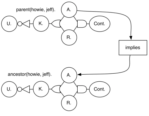
2. We must connect the relevant belief in any matching proposition to belief in its consequent (as evaluated in the environment created by the matching the antecedent). In short, we must create an instance of the rule by binding any variables in the rule to the corresponding terms in the matching proposition. Since we have matched parent(a, b) with parent(howie, jeff), we have obtained the relevant bindings a = howie and b = jeff. Thus, we may consider a specific instance of the parent-ancestor rule parent(howie, jeff) → ancestor(howie, jeff). Given the nature of this rule, there is necessarily a connection between the acceptance of the former proposition of parenthood and acceptance of the latter proposition of ancestry. As a result, we must connect the two belief cells of the propositions such that an affirmative (true) belief in accepting the proposition parent(howie, jeff) will propagate, with its set of premises to the acceptance of the proposition ancestor(howie, jeff), as depicted in Figure 4-1.
Cont. U. K. R. A. Cont. U. K. R. A. parent(howie, jeff). ancestor(howie, jeff). implies
Figure 4-1: A simple network of propositions which propagates the belief in the acceptance of parent(howie, jeff) along with its dependencies to the acceptance of ancestor(howie, jeff). The “implies” propagator ensures that this belief is properly propagated without modification and merged with the contents of the output cell.
(define (prove-ancestry-by-parenthood a b)
(let ((parent-proposition (proposition `(parent ,a ,b))) (ancestor-proposition (proposition `(ancestor ,a ,b)))) (accept ancestor-proposition
(list 'prove-ancestry-by-parenthood a b) (list (accepted parent-proposition)))))
Figure 4-2: Proving ancestry through parenthood. (ancestor a b) is accepted
contingent on (parent a b) being accepted, by way of the
We might represent such a “parenthood” rule using MIT/Scheme code like that of
Figure 4-2. In the function prove-ancestry-by-parenthood, two propositions are
retrieved: parent-proposition (i.e. (parent a b)), and ancestor-proposition
(i.e. (ancestor a b)). With these two propositions in hand, the accept function
states that ancestor-proposition will be believed to be accepted, as informed by
(i.e. caused by) (list ’prove-ancestry-by-parenthood a b). That is, we will
potentially accept (ancestor a b) by way of the fact that we attempted to prove
ancestry through parenthood (with the specified arguments a and b).
This acceptance is not a foregone conclusion, however; the accept function also
states, through its third argument, that this acceptance is based on the acceptance
of parent-proposition. While we may believe (ancestor a b) to be accepted for
any number of reasons, we can only believe it is accepted due to parenthood if we
also believe that we accept (parent a b).
4.2
Knowing the Unknown
While the above example is perfectly acceptable should we know a and b, what if we do not? As stated above, the rule ∀a, b.parent(a, b) → ancestor(a, b) does not require us to know a and b. Indeed, it is true for all a and b. Would it not be better to be aggressive and proactively find parents, so as to prove ancestry without having to be told which ones we are looking for?
There are several problems which must be surmounted with such an approach. The
most obvious difficulty is that of finding all such propositions that match (parent
a b). While we can certainly use efficient database storage and indexing algorithms
to find all such (parent a b) that exist when we are given the rule, we must also
be aware that it is very unlikely that we know all parenthood relationships at that particular point in time. Furthermore, if a system is intelligent enough to know the generic existence of parents (in short, parent(b, c) → ∃a.parent(a, b)), then a system may easily get lost simply proving the existence of parents ad infinitum rather than discovering a relevant ancestry relationship.
Even lacking such a general rule, from a pragmatic standpoint it is also quite
possible that we may not know about certain (parent a b) relationships at a given
time, due simply to their current “irrelevance.” In other words, at any given point there are unknown unknowns; not only do we not know whether we accept or reject
some arbitrary (parent a b), but there are (parent a b) propositions of which we
are not even remotely aware!
Thus, when making such a pattern matcher, we must take care that it is lazy. Any attempt to prove ancestry through the existence of a parenthood relationship must be ready to be acted on at any time, as new parenthood relationships are introduced and believed to be true. That is, we must be prepared to make the connections between propositions asynchronously, by making such connections in callbacks which are invoked whenever such a statement is generated. Thus, we elaborate the code as in Figure 4-3, which pushes the connection of the “acceptance” belief cells into
the function accept-ancestor-by-parenthood. This function may be called when
a matching proposition is found.
Note that here we replace the instantiation of a proposition (parent a b) with
the find-proposition-matching function. This function searches for propositions
matching the pattern(parent ?a ?b), where the question marks denote named
vari-ables a and b. Upon finding any such proposition,accept-ancestor-by-parenthood
is called, with a first argument containing the matching proposition, and a second argument containing a mapping of the variable names to the values resulting from matching the pattern with the proposition.
For example, given the proposition (parent howie jeff), the parent-proposition
variable would contain the proposition itself, while the contents of the environment
variable could be used to determine that the variable ?a would be bound to howie
and the variable ?b would be bound to jeff.
These environmental bindings are used in instantiate-proposition, in which
they are substituted for the ?a and ?b variables in the pattern (ancestor ?a ?b)
to instantiate the proposition (ancestor howie jeff). Then, the acceptance of
;; This function is called with a proposition matching the pattern ;; (parent ?a ?b) and an environment that contains the values that ;; matched the pattern variables ?a and ?b. It then accepts the
;; corresponding (ancestor ?a ?b) proposition contingent on acceptance ;; of the parent proposition.
(define (accept-ancestor-by-parenthood parent-proposition environment)
;; In order to accept the corresponding ancestry proposition ;; (ancestor ?a ?b) we create the proposition by using the ;; environment to fill in ?a and ?b...
(let ((ancestor-proposition
(instantiate-proposition '(ancestor ?a ?b) environment))) ;; We then accept ancestor-proposition based on ?a being the ;; parent of ?b, so long as we accept the proposition
;; (parent ?a ?b)
(accept ancestor-proposition
(list 'prove-ancestry-by-parenthood
(get-binding '?a environment) ; Get value of ?a
(get-binding '?b environment)) ; Get value of ?b (list (accepted parent-proposition)))))))
;; Find propositions matching (parent ?a ?b) and call
;; accept-ancestor-by-parenthood for each such proposition. (define (prove-ancestry-by-parenthood)
(find-proposition-matching '(parent ?a ?b) '() accept-ancestor-by-parenthood))
Figure 4-3: Proving ancestry through parenthood generally. For every (parent ?a
?b) that is known, (ancestor ?a ?b) is accepted contingent on that (parent ?a ?b) being accepted, by way of the “prove-ancestry-by-parenthood” rule. Note the introduction of the environment variable which contains the variable bindings to a and b.
(define (prove-ancestry-by-parenthood)
(find-proposition-matching '(ancestor ?a ?b) '() (lambda (prop-1 environment)
(find-proposition-matching '(ancestor ?b ?c) environment (lambda (prop-2 environment)
(let ((ancestor-proposition (instantiate-proposition '(ancestor ?a ?c)
environment))) (accept ancestor-proposition
(list 'prove-ancestry-transitively (get-binding '?a environment) (get-binding '?b environment) (get-binding '?c environment)) (list (accepted prop-1)
(accepted prop-2)))))))))
Figure 4-4: Proving ancestry through transitivity. For every(ancestor ?a ?b) and
(ancestor ?b ?c) that is known, (ancestor ?a ?c) is accepted contingent on those two previous ancestor relationships being accepted, by way of the “prove-ancestry-transitively” rule. Note how the environment variable is carried as an argument to
the nested find-proposition-matching function, and how it implicitly carries the
bindings of the named variable a through to the inner lambda in which the proposition (ancestor ?a ?c) is instantiated.
as in Figure 4-2. Similarly, the get-binding function must be used to resolve the
bindings to ?a and ?b. In this way, the explanation of the method used to conclude
acceptance may be constructed.
The observant reader will note that the find-proposition-matching function
takes an empty list as its second argument. A second argument is helpful when mul-tiple patterns are chained together, as in the ancestor-chaining rule implemented in
Figure 4-4. As the variable?b must be the same value in both (ancestor ?a ?b) and
(ancestor ?b ?c) in order to prove ancestry through transitivity, the environmental bindings created by matching the former must be passed to the latter so as to
par-tially instantiate the pattern (ancestor ?b ?c) with the known value of ?b. Thus,
the second argument acts as an environment in which to evaluate the pattern before performing a search, and the empty list merely denotes an empty initial environment containing no variable bindings.