Dynamics of global ocean heat transport variability

Dynamics of Global Ocean Heat Transport Variability

Steven Robert Jayne

S.B., Massachusetts Institute of Technology (1994)

Submitted in partial fulfillment of the requirements for the degree of

DOCTOR OF SCIENCE at the

MASSACHUSETTS INSTITUTE OF TECHNOLOGY and the

WOODS HOLE OCEANOGRAPHIC INSTITUTION February 1999

®

The author hereby grants to MIT and WHOI permission to reproduce paper and electronic copies of this thesis in whole or in part, and to distribute them publicly.

Signature of Author

Joint Program in Physical Oceanography Massachusetts Institute of Technology/ Woods Hole Oceanographic Institution

February 27, 1999

Certified by.

N...

Dynamics of Global Ocean Heat Transport Variability by

Steven Robert Jayne

Submitted to the Massachusetts Institute of Technology/Woods Hole

Oceanographic Institution Joint Program in Oceanography/Applied Ocean Science and Engineering in partial fulfillment of the requirements for the degree of

Doctor of Science in Oceanography. February 27, 1999

Abstract

A state-of-the-art, high-resolution ocean general circulation model is used to es-timate the time-dependent global ocean heat transport and investigate its dynamics. The north-south heat transport is the prime manifestation of the ocean's role in global climate, but understanding of its variability has been fragmentary owing to uncer-tainties in observational analyses, limitations in models, and the lack of a convincing mechanism. These issues are addressed in this thesis.

Technical problems associated with the forcing and sampling of the model, and the impact of high-frequency motions are discussed. Numerical schemes are suggested to remove the inertial energy to prevent aliasing when the model fields are stored for later analysis.

Globally, the cross-equatorial, seasonal heat transport fluctuations are close to +4.5 x 1015 watts, the same amplitude as the seasonal, cross-equatorial atmospheric energy transport. The variability is concentrated within 200 of the equator and dom-inated by the annual cycle. The majority of it is due to wind-induced current fluctu-ations in which the time-varying wind drives Ekman layer mass transports that are compensated by depth-independent return flows. The temperature difference between the mass transports gives rise to the time-dependent heat transport.

The rectified eddy heat transport is calculated from the model. It is weak in the central gyres, and strong in the western boundary currents, the Antarctic Circumpolar Current, and the equatorial region. It is largely confined to the upper 1000 meters of the ocean. The rotational component of the eddy heat transport is strong in the oceanic jets, while the divergent component is strongest in the equatorial region and Antarctic Circumpolar Current. The method of estimating the eddy heat transport from an eddy diffusivity derived from mixing length arguments and altimetry data,

and the climatological temperature field, is tested and shown not to reproduce the model's directly evaluated eddy heat transport. Possible reasons for the discrepancy are explored.

Thesis Supervisor: Dr. Jochem Marotzke Associate Professor of Physical Oceanography

Department of Earth, Atmospheric, and Planetary Sciences Massachusetts Institute of Technology

-Acknowledgments

I would like to gratefully acknowledge my advisor Jochem Marotzke for guidance, encouragement and the freedom to pursue a thesis topic not necessarily what he had envisioned. I would also like to thank my thesis committee members Nelson Hogg, Paola Malanotte-Rizzoli, Breck Owens and Carl Wunsch for their advice and suggestions which helped shape this research. Bruce Warren kindly agreed to chair my thesis defense.

Special thanks are due to Robin Tokmakian and Bert Semtner from the Naval Postgraduate School, who generously provided their numerical model output. Robin gave me considerable help and advice on working with the model output and provided me with the wind stress and surface heat flux fields used to force the model. Thanks are due to Charmaine King for providing me with the gridded TOPEX/POSEIDON fields. The Scientific Computing Division at the National Center for Atmospheric Research also gave invaluable technical consulting and made the processing of over 250 gigabytes of model output and data feasible. Jim Price and Breck Owens also provided computer resources. Thanks to Alistair Adcroft for providing the Laplacian inverter, Rui Ponte for critical advice on angular momentum calculations, Mike Spall for providing comments on Chapter 2 and Mindy Hall for comments on what became Chapter 4.

I would like to thank all my friends from WHOI and MIT; I have been fortunate to have so many good friends, you have given me the moral support to get through graduate school. In particular I would like to give heartfelt thanks to David Ford, Ryan Frazier, Chris Linder, Liz Kujawinksi, Sean McKenna, Jess Rowcroft, Sarah Walsh and Joe Warren for the good times and encouragement, you all made grad school fun. I also thank my fellow PO students; Jay Austin, Derek Fong, Frangois Primeau, Jamie Pringle, Louis St. Laurent and Judith Wells for their years of help and comradeship. I would also like to thank the folks in the Education Office for their efforts to make graduate school as painless as possible.

Finally, though it is surely an inadequate expression of my gratitude, I thank my parents for all their support. It is they who have made all this possible, and to whom

I can finally say, I'm done with school.

Funding for this research came from the Department of Defense under a National Defense Science and Engineering Graduate Fellowship. Financial support was also contributed by the National Science Foundation through grants #OCE-9617570 and #OCE-9730071, and the Tokyo Electric Power Company through the TEPCO/MIT Environmental Research Program. The author received partial support from an MIT Climate Modeling Fellowship, made possible by a gift from the American Automobile Manufacturers Association. The computational resources for the numerical simu-lations where provided by the National Center for Atmospheric Research which is supported by the National Science Foundation and operated by the University Cor-poration for Atmospheric Research. This thesis was brought to you by the letter D and the number 7.

"To know the laws that govern the winds, and to know that you know them, will give you an easy mind on your voyage round the world; otherwise you may tremble at the appearance of every cloud. What is true of this in the trade-winds is much more so in the variables, where changes run more to extremes"

Joshua Slocum (1844-1909)

Contents

Abstract

Acknowledgments 1 Introduction

2 Forcing and Sampling of Ocean General Circulation Models: of High Frequency Motions

2.1 Introduction . . . . 2.2 Changes in the forcing of the model ...

2.3 Solutions to aliasing of the inertial frequencies . . . . 2.3.1 Average fields . . . . 2.3.2 Ham m ing filter . . . . 2.4 C onclusions . . . . 2.5 Appendix: Derivation of interpolation spectra . . . .

Dynamics of Wind-Induced Heat Transport Introduction . . . . T he m odel . . . . The seasonal cycle in meridional overturning . . . The seasonal wind field . . . . Linear homogeneous shallow water model . . . . . 3.5.1 Free surface height deviations . . . . Meridional overturning . . . . Adjustment to variable wind stress . . . .

Impact 19 . . . . 19 . . . . 21 . . . . 26 . . . . 29 . . . . 29 . . . . 34 . . . . 35 Variability 43 . . . . 43 . . . - - . . 47 . . . . 48 . . . . 56 . . . . 61 . . . . 63 . . . . 67 ... . . . 71 3 The 3.1 3.2 3.3 3.4 3.5 3.6 3.7

3.7.1 The equator . . . . 3.7.2 A summary of the ocean's response 3.8 Implications for heat transport . . . .

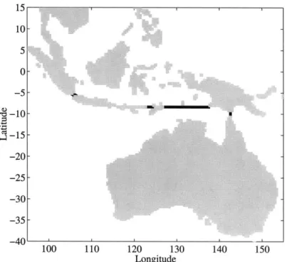
3.8.1 Indo-Pacific throughflow . . . . 3.8.2 Seasonal heat transport variations . 3.8.3 The tropics . . . . 3.8.4 Error estimates . . . . 3.9 Discussion and conclusions . . . .

. . . . time-varying wind . . . . . . . . . . . . . . . . . . . . . . . .

4 Ocean Heat Transport Variability

4.1 Introduction . . . . 4.2 Time-mean heat transport . . . . 4.3 Comparison of the annual cycle with previous model results servational evidence. . . . . 4.4 Basin heat transport variability . . . . 4.5 Temporal decomposition . . . . 4.6 Dynamical decomposition . . . . 4.7 The seasonal heat balance . . . . 4.8 Rectified variability . . . . 4.8.1 A meandering jet . . . . 4.8.2 The global distribution of eddy transport . . . . 4.8.3 Frequency distribution . . . . 4.9 Discussion and conclusions . . . . 5 Summary and Conclusions

5.1 Summary of results . . . . 5.2 Concluding remarks . . . . stress and ob-76 78 79 80 83 90 90 92 95 95 97 100 104 110 114 120 124 129 138 148 149 153 . . . . . 153 . . . . . 158 Bibliography ₁₆₁

Chapter 1

Introduction

The Earth's climate is a dynamic system and the turbulent circulations of the ocean and atmosphere participate in a complicated exchange of heat, mass, and momentum. The complexity of this system coupled with sparse observational coverage of it has made interpretation and understanding of some of the underlying processes difficult. Further, its intricacies limit our ability to predict anthropogenic impacts on climate. The ocean component of it still presents some of the largest gaps in our knowledge of the fundamental processes involved. In this thesis I approach some of the questions concerning the ocean's role in climate by addressing the role of temporal variability in the ocean's transport of heat, and in particular, the global nature of the relevant ocean dynamics will be investigated.

Estimates of the time-mean ocean heat transport show that the ocean carries the same order of magnitude of energy away from the tropics towards the poles as the atmosphere (Vonder Haar and Oort 1973; Hastenrath 1982; Carissimo et al. 1985; Peixoto and Oort 1992; Trenberth and Solomon 1994; Keith 1995). Macdonald and Wunsch (1996) made a dynamically and kinematically consistent estimate of the global transports of mass, heat, and freshwater based on an inverse model of a collection of one-time hydrographic sections. With the completion of the World Circulation Experiment (WOCE) more hydrographic sections are now available and a better estimate will be possible. Contributions to the understanding of the ocean heat transport have come from modeling studies as well (for a summary see Bryan 1991). While uncertainties still exist in estimates of the time-mean ocean heat transport, in

general it can be said that at least the sign of the ocean heat transport is known over the global ocean and quantifiable error estimates can be made.

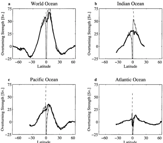
Overall in the time-mean picture the ocean, as does the atmosphere, transports heat away from the tropics toward the polar regions, helping to balance the unequal heating of the Earth by the Sun and moderate temperatures at both extremes. The heat transport in the Atlantic Ocean is toward the north over its entire latitudinal extent, consistent with simple conceptual models for the thermohaline circulation by the global ocean (Broecker 1991). Elsewhere, in the Pacific Ocean there is poleward transport of heat away from the equator, and in the Indian Ocean there is southward heat transport over the basin's extent.

Keith (1995) concluded that the time-mean ocean heat transport calculated as the residual to close the atmospheric energy budget, has achieved the same accuracy as direct hydrographic methods. Though the uncertainties in the transports may be as large as 0.7 PW (1 PW = 1015 watts) and errors still remain in the partition between the ocean and atmosphere, the estimates are believed to be good enough to constrain coupled ocean-atmosphere climate models. Since the time-mean heat transport has been reasonably, though not completely addressed, it is timely to con-sider its time-dependent nature, which is important for several reasons. There is energetic variability in the ocean due to mesoscale eddies, wave motions, atmospheri-cally driven transients, etc. First, the nature and magnitude of the time-dependency of the ocean heat transport is not well known and conflicting estimates of it exist and it therefore represents a large gap in our understanding. Second, it may or may not impact our ability to observe the time-mean transport. How much the rectified temporal variability contributes to the time-mean heat transport, and whether the variability significantly impacts estimates of the time-mean state made from one-time hydrographic sections, remain open questions.

Direct observation of the time-dependent heat transport by the ocean on any reasonable timescale is prohibited by the impossibility of sampling the full ocean depth over the vast range of spatial scales required. Though hydrographic surveys do provide some measure of the eddy variability along the section, it is strongly aliased in time. Therefore, estimates of the global variability have had to rely on indirect

approaches. These have been based on models (Bryan and Lewis 1979; Bryan 1982) or observed changes in oceanic heat storage, combined either with atmospheric and satellite observations (Oort and Vonder Haar 1976; Carissimo et al. 1985), surface flux observations (Hsiung et al. 1989) or wind-stress and surface temperatures to estimate changes in the Ekman component of the heat transport (Kraus and Levitus 1986; Levitus 1987; Adamec et al. 1993; Ghirardelli et al. 1995).

The seasonal cycle of ocean heat transport has been the subject of several in-vestigations. This was begun by Oort and Vonder Haar (1976), who used satellite radiation data, atmospheric radiosonde data and oceanic heat storage data to study the ocean heat transport in the Northern Hemisphere. Their method calculated the ocean heat transport as the residual necessary to close the energy balance at the top of the atmosphere, after accounting for atmospheric and oceanic heat storage and atmospheric transport. They inferred a large seasonal variation in the ocean heat transport particularly in the tropics where they found that the oceans transport large amounts of heat across the equator from the summer hemisphere to the win-ter hemisphere. Carissimo et al. (1985) essentially updated the study of Oort and Vonder Haar (1976) using data covering the entire globe. They too found a large seasonal variation in the ocean's inferred heat transport. Peak to peak, their annual cycle of heat transport across the equator was 7.3 t 4 PW. Over the mid-latitudes, the amplitude was smaller, but still directed northward during boreal winter (austral summer) and southward during boreal summer (austral winter). The large errorbars on this estimate are largely due to the poor quality and general lack of ocean heat storage data available at the time of their study.

Kraus and Levitus (1986) calculated the annual heat transport variations across the Tropics of Cancer and Capricorn by the Ekman heat transport and found that the amplitude of the annual cycle was the same order of magnitude as the annual mean Ekman heat transport in both the Pacific and Atlantic Oceans. This work was extended by Levitus (1987) who calculated the Ekman heat transport for all three ocean basins over their latitudinal extents using a climatological data set for the temperature (Levitus 1982) and wind stress (Hellerman and Rosenstein 1983) fields. The essential premise of these calculations is that the atmospheric wind stress drives

an Ekman transport in the surface layer which is accompanied by a compensating return flow which is distributed barotropically. Since the return flow is at the depth averaged temperature, which is generally colder than the surface temperature, there is a heat transport proportional to the temperature difference and the zonal wind stress. More recently Adamec et al. (1993) used wind stress values and tempera-tures computed from the Comprehensive Ocean-Atmosphere Data Set (COADS) to compute the Ekman heat transport. Ghirardelli et al. (1995) used satellite derived wind stress from the Special Sensor Microwave Imager (SSM/I) and sea surface tem-perature from the Advanced Very High Resolution Radiometer (AVHRR). All these studies qualitatively give the same picture of the annual cycle of the Ekman heat transport. Over the World Ocean the annual cycle is of order 8 petawatts peak to peak in the tropics. It is strongest in the Pacific and Indian Oceans and noticeably weaker in the Atlantic Ocean. Additionally, the phase of the annual cycle reverses in the mid-latitudes at around 200. There are, however, some difficulties interpreting the role of the Ekman heat transport in climate processes from these studies. First, the Ekman heat transport is only one component of the total transport; changes in it may be unaffected, reinforced or completely offset by changes in other parts of the system. Second, none of these studies is applicable within a few degrees of the equator as their definition of the Ekman transport breaks down with the vanishing Coriolis parameter there. Third, none of these investigations can take into account Bryan's (1982) finding that the meridional wind plays an increasingly important role as one approaches the equator. Finally, these studies are sensitive to the assumed return flow temperature and all combine the time-dependent Ekman transports with the time-mean Ekman transport assuming that both flows have the same depth struc-ture. The assumption that the return flow for the time-varying Ekman transport is deep and barotropic, is supported superficially by theory (Willebrand et al. 1980) and modeling studies (Bryan 1982; B6ning and Herrmann 1994), but a solid dynamical argument is needed. Furthermore, there is neither a theoretical, nor an observational, nor a modeling basis to assume that the time-mean Ekman transport should be re-turned barotropically. In fact, Anderson et al. (1979) and Willebrand et al. (1980) clearly indicate that a time-mean forcing drives a circulation which is strongly

influ-enced by stratification and nonlinear effects and is generally not barotropic. More recently, Klinger and Marotzke (1999) have argued that the time-mean Ekman layer mass transport is returned at relatively shallow depths. Given a typical ocean tem-perature distribution, a shallower return flow translates into a warmer return flow and decreases the strength of the heat transport compared to a deep barotropic return flow. Therefore, while the time-dependent portions of the Ekman heat transports are reliable estimates, the time-mean component should be viewed with suspicion.

Global ocean general circulation models were used by Bryan and Lewis (1979), Bryan (1982) and Meehl et al. (1982) to explore heat transport variability. Bryan and Lewis found a significant seasonally varying heat transport, whose structure and amplitude was similar to that found by Hsiung et al. (1989). Meehl et al. (1982) added a seasonally varying, surface heat flux forcing to a similar ocean model and used a wind stress field which had both a semiannual harmonic and an annual harmonic. Their results were similar to those of Bryan and Lewis (1979) for the seasonally varying heat transport, with the addition of a semi-annual signal in the heat transport due to the different forcing fields. Lau (1978) also found a large annual cycle in the ocean heat transport, but did not directly attribute it to the seasonal wind stress cycle. Bryan (1982) found that while the zonal wind stress seasonal cycle forced an ocean heat transport from the summer hemisphere to the winter hemisphere, the seasonal cycle in the meridional wind acted to suppress the heat transport seasonal cycle in the tropics. This was particularly true close to the equator where a meridional surface layer transport can be driven directly by the meridional wind, owing to the Coriolis parameter going to zero there. Bryan's (1982) seminal explanation of the physics behind the seasonally varying Ekman flows, which are the major source of ocean heat transport variability, seems to have been largely ignored outside of the ocean modeling community. More recently, models of various resolutions have been applied to basin-scale studies. B6ning and Herrmann (1994) and Yu and Malanotte-Rizzoli (1998) have examined the Atlantic Ocean, while McCreary et al. (1993), Wacongne and Pacanowski (1996), Garternicht and Schott (1997) and Lee and Marotzke (1998) looked at the Indian Ocean. These studies all found strong annual cycles in the ocean heat transport and confirmed the importance of the wind on the ocean heat transport

variability. The Pacific Ocean has not been investigated and there have been no recent model studies of the global, time-dependent ocean heat transport with high resolution since Bryan (1982) and Meehl et al. (1982). Further, all the above works use monthly wind stress fields and it is unknown whether higher frequency wind stress fields will introduce high frequency ocean heat transport oscillations.

The most recent global estimate of the time-mean and seasonal cycle of ocean heat transport was made by Hsiung et al. (1989) using ocean heat storage data calculated from the Master Oceanographic Observations Data Set (MOODS). They closed their energy budget at the ocean surface with fluxes computed using the bulk formulae. The ocean heat transport was calculated as the residual needed to close the energy budget in the ocean after accounting for surface fluxes and storage terms. This work expanded that of Lamb and Bunker (1982) in the Atlantic to cover the Pacific and Indian Oceans as well. Their estimate of the annual cycle of heat transport across the equator by the ocean had a peak to peak amplitude of 4.4 ± 1.4 PW. Overall, the picture of the annual cycle they presented was consistent with that of Bryan (1982). However, they found the annual cycle lagged several months behind that of Carissimo et al. (1985). Hsiung et al.'s (1989) seasonal cycle reversed sign in mid-latitudes, as in the studies of Ekman heat transport discussed above, as well as in those of Bryan and Lewis (1979) and Bryan (1982). Therefore, from previous studies there appears to be a large seasonal cycle driven by the seasonal cycle of wind stress. However, there is disagreement about both its magnitude and dynamics. The global studies by Hsiung et al. (1989), Bryan (1982) and Levitus (1987) give a generally consistent picture of the seasonal heat cycle, though differing in details. In contrast, the study of Carissimo et al. (1985), stands out as significantly different from the other estimates, most likely because their data was not sufficiently precise to resolve the seasonal cycle in ocean heat transport.

There are additional consequences of the ocean heat transport variability to be considered. One of the uses for hydrographic surveys, either single lines or large international programs such as the World Ocean Circulation Experiment (WOCE), is that the annual-mean ocean heat transport at a latitude can be estimated by a one-time ocean section. These estimates of heat transport rely on the method used by

Hall and Bryden (1982) or on global inversions of hydrographic data (Macdonald and Wunsch 1996). However, if there is strong ocean variability, the estimate of the heat transport may be badly corrupted. Hall and Bryden (1982) assessed the potential error introduced by eddy noise on their estimate of the heat transport at 24'N and found that it could be as large as 25% of the total and was the largest error in their estimate. Additionally, seasonal biases may corrupt estimates of heat transport owing to the predominance of summer time oceanographic field work, particularly at high latitudes. Therefore, it is important that the ocean heat transport variability be quantified and its impact on hydrographic heat transport estimates be evaluated.

Finally, the time-varying circulations themselves can contribute to the mean ocean heat transport by rectification. This process is the subject of considerable interest and debate. Coarse resolution models do not resolve the transport processes asso-ciated with the oceanic mesoscale field. Therefore, significant effort has been spent developing a parameterization of the mesoscale eddy field (e.g. Gent and McWilliams 1990; Holloway 1992; Griffies 1998). However, the role of the oceanic mesoscale eddy field in climate processes has been only marginally addressed observationally. Stam-mer (1998) used altimetry data from the TOPEX/POSEIDON satellite to estimate mixing length scales over the global ocean, and combined them with a climatological temperature field to estimate the eddy heat transport by the ocean. He found that over large areas of the ocean gyres the eddy heat transport was small. But, in several places the eddy heat transport was significant: the western boundary currents, the equatorial regions and the Antarctic Circumpolar Current. Wunsch (1999) using a compilation of current meter data came to a similar conclusion. However, the ques-tion of whether mixing length scales are even appropriate to parameterize the effects of the ocean mesoscale eddy field has not been addressed using direct ocean mea-surements, though analyses of atmospheric data suggest they work in the atmosphere (Kushner and Held 1998).

Enhanced computational capability over the past 20 years has allowed ocean gen-eral circulation models to use significantly higher resolution than Bryan and Lewis (1979) used in their global ocean model with approximately 2.5' resolution to look at the seasonal variation in poleward heat transport. Resolution has increased by over

an order of magnitude from that in Bryan and Lewis's (1979) calculations. Addition-ally, more accurate and higher frequency wind stress fields are now produced by the meteorological centers such as the European Centre for Medium-Range Weather Fore-casting (ECMWF) and the National Centers for Environmental Prediction (NCEP) and improved fields of surface heat and freshwater flux are available (Barnier et al. 1995). These factors taken together make current numerical model simulations more realistic than their predecessors.

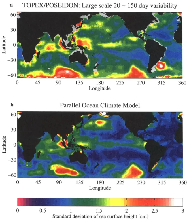
This thesis addresses the dynamics of the time-dependent ocean heat transport through the use of a state-of-the-art ocean general circulation model. Specifically, output from the Parallel Ocean Climate Model from the Naval Postgraduate School is used (the POCMAB run was discussed by Stammer et al. (1996) and McClean et al. (1997)). The model is a primitive equation, level model (Semtner and Chervin 1992). It has an average resolution of 1/4' in the horizontal direction, and 20 levels in the vertical. It uses realistic topography and extends over a domain from 750S to 65'N. The model output is available at 3-day intervals throughout the model run. The output was instantaneously sampled from the model and not averaged or filtered, creating temporal aliasing problems (Jayne and Tokmakian 1997; and Chapter 2 of this thesis). The ability of this particular numerical simulation to represent the true variability of the ocean has been addressed by Stammer et al. (1996) and McClean et al. (1997).

Using a high-resolution global ocean general circulation model allows insight into the nature and magnitude of the seasonal cycle of the ocean heat transport. The behavior of higher frequency oscillations can be examined as well. It is also possible to determine the magnitudes of the variability induced by mechanisms other than the Ekman heat transport. Though the use of a numerical model suffers from the model's dependencies and deficiencies, it does let us test dynamical theories for the physical mechanisms that drive the ocean heat transports inferred by Carissimo et al. (1985) and Hsiung et al. (1989). It will also permit an examination of the frequency range higher than the seasonal cycle which heretofore has not been addressed by other modeling studies. Furthermore it allows a more complete picture of the total heat transport variability than can be garnered from examining only the Ekman

contribution to the heat transport and allows us to check the consistency of the assumptions that go into the estimates of the Ekman heat transport. It allows an assessment of the contribution of mesoscale eddies to the time-mean heat transport and their impact on one-time hydrographic sections. Most important, it gives a global picture of all these processes that has been heretofore lacking.

Bearing in mind that the model which I have chosen to analyze is not a perfect representation of the ocean and may have significant errors, it is still useful for eluci-dating the physical mechanisms which lead to heat transport variability in the ocean. Chapter 2 of this thesis addresses the appropriate forcing and sampling of ocean models in which high-frequency motions are present. The nature of aliasing of the high-frequency phenomena given varying sampling methods is discussed and schemes are provided that will remove the aliased energy from the model fields stored for later analysis. A reader who is uninterested in the technical details of this problem may skip this chapter. A complete theory for the role of variable wind stress in forcing fluctuating ocean heat transport has been lacking. While some of the underlying dy-namics have been discussed in previous studies, they have never been put together in a cohesive argument. Chapter 3 examines the dynamics allowing temporal variations in wind stress to lead to large variations in the ocean heat transport. These arguments are illustrated with a conceptual model and a homogeneous, shallow-water model with full topography and wind forcing. A detailed description of the time-dependent nature of the ocean heat transport as seen in the Parallel Ocean Climate Model is described in Chapter 4. The time variations in the heat transport are broken down into components due to velocity variations, temperature variations and the covaria-tion of temperature and velocity. Addicovaria-tionally, the heat transport is decomposed into dynamical components, separating the Ekman, gyre and baroclinic contributions to the heat transport variability and allowing an analysis of the impact of the temporal variability on estimates of the time-mean heat transport from hydrographic sections. Finally, the rectified eddy heat transport from the POCM is discussed. A comparison with an analysis derived from TOPEX/POSEIDON data (Stammer 1998) is made and the validity of using a mixing length hypothesis to derive the eddy heat transport is tested.

Chapter 2

Forcing and Sampling of Ocean

General Circulation Models:

Impact of High Frequency Motions

Steven R. Jayne and Robin Tokmakian 1

2.1

Introduction

Inertial oscillations arise as simple solutions to the momentum equations for a rotating fluid. In the ocean, these motions are known to be energetic and it should therefore not be surprising that they are significant in numerical models of the ocean driven by realistic, high-frequency forcing. Long time series of realistic wind stress fields are now available 4 times per day for forcing ocean general circulation models (OGCM) and therefore the effects of associated inertial oscillations present in the models on model diagnostics need to be addressed. Two problems arise with respect to inertial oscillations in OGCMs. First, the temporal approximation form of the wind stress forcing can excite zonal bands of large amplitude oscillations. For example if wind fields are not changed smoothly in time but are updated every 3 days, the step function resonantly forces the inertial oscillations at specific latitudes. Secondly, most analyses of OGCM output for climate research or process studies are unconcerned

'This chapter is adapted from the paper which appeared in Journal of Physical Oceanography, June 1997, volume 27, pages 1173-1179. @ 1997 American Meteorological Society. Reprinted with

permission. Woods Hole Oceanographic Institution contribution number 9355. Figure 2.4b and the appendix did not appear in the published paper, but are included here for completeness.

about processes at timescales that are as short as the inertial period. However, if the prognostic fields are sampled at any interval greater than half the inertial period, instantaneous sampling will alias inertial oscillations into lower frequencies that vary with latitude.

Recent analysis of high resolution primitive equation models (Parallel Ocean Cli-mate Model (POCM) with 1/40 resolution (Semtner and Chervin 1992; Stammer et al. 1996) and Los Alamos Parallel Ocean Project (POP11) with 1/60 resolution (Dukowicz and Smith 1994; Fu and Smith 1996)) as well as lower resolution OGCMs (e.g. the global MIT model with 1' resolution (Marshall et al. 1997a; Marshall et al. 1997b)) all show unrealistic features in the output velocity fields (u and v) subsam-pled every 3 days and the associated diagnosed field of eddy kinetic energy (EKE) which result from the aliasing of inertial oscillations generated by the high-frequency wind stress forcing fields. To understand and to remove this unrealistic signal from future model runs, we have analyzed the sensitivity of the model inertial motions and the model output on the temporal forcing and the sampling period. Both aspects are addressed in this chapter. To do so, the temporal forcing was changed from unin-terpolated step functions to a linear interpolant of the data. The sampling scheme is modified to filter out oscillations at frequencies higher than the Nyquist frequency prior to the model fields being saved to output.

Tests are performed using the 1/4' resolution POCM. The version of the model is the same as described by Stammer et al. (1996). It is a primitive equation model on a Mercator grid (nominal resolution of 1/4') with 20 levels in the vertical. The model's surface momentum is forced with realistic wind stress fields derived from the twice-daily European Centre for Medium-Range Weather Forecasting (ECMWF) 10 m wind fields. The resulting wind stress fields are interpolated in space using bi-cubic spline fits onto the model grid. The changes of the present runs relative to the standard run discussed by Stammer et al. (1996) are related to 1) the temporal wind forcing and 2) the sampling of the prognostic variables, which are summarized in Table 1. All runs were initiated from the same point in time, February 23, 1993, defined by the date of the ECMWF wind stress fields and the initial prognostic 3-D model fields from the run of POCM 4_13. Sampling of POCM 4_13 was instantaneous

Table 2.1: Summary of test runs with varying forcing periods, functional forms, and sam-pling periods.

Test number Wind forcing Interpolation Sampling Original (POCMAB) 3 day no 3-day snapshot

1 3 day no hourly

2 3 day linear hourly

3 1 day linear hourly

snapshots of the model's prognostic variables (velocities, temperature, salinity and sea surface elevation) every 3 days. The model time step is 1/2 hour. In this study, the model's prognostic variables were also sampled hourly along several lines, meridional and zonal, to determine the differences resulting from how each run was being forced. For POCM 4_B and test 1, the wind stress fields were held constant over a 3 day period, whereas for tests 2 and 3 the wind stress fields were linearly interpolated to each time step. Section 2 focuses on the forcing problem and section 3 discusses the possible remedies to remove the aliasing in the sampled fields.

2.2

Changes in the forcing of the model

Inertial oscillations are a well studied phenomenon in the ocean (Fu 1981; Gill 1982). A simple model of inertial oscillations can be found by a reduction of the momentum equations:

Du

- fv = Tr(t) - ru

at _(2.1)

+ fu = rT (t) - rV,

where u is the zonal component of velocity and v is the meridional component of velocity,

f

#

dissipation. This coupled set of differential equations can be solved to give:

where i = -. This solution has a strong resonance at the frequency -f which is limited only by the presence of dissipation so any energy in the forcing at that frequency will excite inertial oscillations of significant amplitude. In a statistical sense, the amplitude response of the inertial oscillations can be understood by knowing the characteristics of the rotary spectrum for the forcing function, r(t). The spectral response, S+io(w), of (2.2) is given by:

Sr (w)

S(+i ) = f-r) 2 _(2.3)

(w + f - ir)2

where w is the angular frequency and S, (w) is the power spectrum of the wind forcing (Priestley 1981).

In the real world, the wind stress varies on all timescales and ST(w) is a continuous function. However, the available high-frequency wind stress data sets are provided at best only 4 times a day as compared to model time steps of about an hour. What is the most appropriate method to interpolate the provided wind fields to the model time steps in such a way as to best preserve the real high-frequency wind stress spectrum? Three methods are possible: 1) a wind stress field kept constant over an observation period (series of step functions), 2) a wind field linearly interpolated between observation time points and 3) a cubic spline interpolation (or other higher-order method, such as Hermite interpolation) of the wind forcing. At frequencies lower than the Nyquist frequency of the wind stress data, the power spectrum of the forcing is determined by the data. However, at frequencies higher than the Nyquist frequency of the data, the power spectrum is dominated by the auto-correlation behavior of the functional form used for the interpolation. If the available data have a Nyquist period that is order days, then the inertial frequency for latitudes away from the equator will lie in the portion of the power spectrum that is determined by the interpolation and accordingly the forcing of inertial oscillations will be a function of the interpolation scheme. If one is not interested in inertial motions, the interpolation method therefore should be chosen carefully so that its high-frequency characteristics are smooth and continuous to avoid artificial high-frequency motions. However, there may be issues related to mixed-layer-physics parameterizations where the inertial energy is needed (Large et al. 1994).

Since most high-frequency wind stress data sets will require some form of interpo-lation to be used as forcing in an OGCM, it is necessary to discuss the implications of various methods. The two methods discussed here are 1) keeping the wind stress constant over a data period since it is relevant to the available POCM output and 2) the more commonly used linear interpolation. In order to establish a notational framework, we first denote a sequence of indices for the forcing functions; where

i = 0, 1, 2, ... are the times when we have data available and

j

the model time steps that we are interpolating the original data to. If the model wind stress is simply updated once per 3 days without any interpolation, the forcing function is written:

rT = ai (2.4)

for all

j

S (w) - cos(wh) sinc2 h, (2.5)

(wh)2 2

where h = 3 days. The more advanced technique of linearly interpolating to each time step between the available data is denoted by:

rf = ai + bj(jAt), (2.6)

where bi = (ai+1 - ai)/h, where ai is again the wind stress read in from the data files

for that day, and aj+1 is the wind stress for the third day following,

At

So

(wh)4 2

It can be seen that both of these methods have zeros in the power spectrum at

of 3 days, 1.5 days, 1 day, etc. Any motions at these periods will be only weakly forced compared with motions with frequencies at wh ~ 37r, 57r, 77r,... (periods of 2 days, 1.2 days, 0.86 days, etc.) which are located at local maxima of both the forcing functions' spectra. If the zeros correspond to the period of the inertial oscillations at a given latitude, there will be a marked decrease in the amplitude of the inertial oscillations at that latitude since there is much less energy in the forcing to drive them. On the other hand if the inertial period is at a local maximum in the power spectrum of the forcing function the inertial oscillations will be forced much more strongly. Moreover, between the zeros in the power spectrum, the peaks fall off at a rate of w 2 for the uninterpolated forcing and w- 4 for the linearly interpolated forcing. This should result in a noticeable depletion in the strength of the inertial oscillations at the latitude where their frequency is higher than the Nyquist frequency of the data and a more general weakening in the high-frequency energy in the model overall.

These effects can be seen in two different ways in the hourly sampled model data. First, we can consider the power spectrum of the velocity at a single point in the ocean as a function of frequency. If the velocities in the surface layer are strongly coupled to the forcing function at high frequencies, it is expected that the shape of the spectrum for the velocities will be strongly influenced by the shape of the forcing spectrum. Figure 2.1 shows the power spectrum of the u component of velocity sampled every hour for the surface layer at 30'N, 200'E for the 3 different forcing tests. Most noticeable is the deficit of energy at frequencies corresponding to 3 days and 1.5 days and peaks of energy at 2 days and 1.2 days when the forcing function is derived from the once-per-3-day data in both the uninterpolated and linearly interpolated methods. The comparison at higher frequencies becomes more difficult owing to the noisiness of the spectrum and to the strong spectral peak from the inertial oscillations. At 30'N the peak in the spectrum due to the inertial oscillations corresponds to approximately 1 day, where a spectral gap from the forcing is expected. But, the energy in the higher frequencies does indeed show an overall weakening of almost an order of magnitude when the linear interpolant is used. This is consistent with the analytic forms derived above. When the wind stress forcing is derived from daily data instead of data every 3 days, the spectrum fills out at periods of longer than 2 days, but now shows a

depletion at the 1-day period, again consistent with the previous arguments if h = 1 day. 10 10 o02 10 10 0 | 1 10 3 lo I 10 0 0 10-4-10-1 10- 10 10,

Cycles per hour

Figure 2.1: Frequency spectra of the u component of velocity at 30'N, 200'E in the North Pacific for tests 1 with once per 3 days uninterpolated forcing (thin solid line), test 2 with once per 3 days linearly interpolated forcing (dashed line) and test 3 with once per day linearly interpolated forcing (heavy solid line). Vertical dashed lines are at the expected minima (3 days and 1.5 days) and dotted lines are the expected maxima (2 days and 1.2 days). The thin solid vertical line is at the inertial frequency.

The second way to compare these analytic arguments to the model results is to consider the amplitude of the inertial oscillations as a function of latitude. Since the frequency of the inertial oscillations increases with increasing latitude, the iner-tial oscillations will be forced by varying energy according to (2.5) and (2.7), and therefore we expect to see minima in the amplitude of the inertial oscillations where S,(w) is small and maxima where it is large. At most latitudes the inertial oscilla-tions dominate the EKE in the hourly sampled data, so we use the EKE as a proxy for the strength of inertial oscillations. Figure 2.2 shows the EKE as a function of latitude for the three tests. Figure 2.2a compares the uninterpolated forcing (test 1) with the linearly interpolated forcing (test 2). The EKE from test 1 shows bands

of sharp peaks alternating with bands of low energy. The bands of low energy cor-respond directly to latitudes where the forcing spectra have minima, namely where

wh

f

asin 2 for n= 1,2, 3,... , (2.8)

which for once-per-3-day data (h = 3 days) occur at the latitudes 9.6 0, 19.40, 29.90,

41.7' and 56.2'. The most noticeable effect from the change to linear interpolation is the significant decrease in strength of the EKE away from the equator when the linear interpolation is used. This is driven by the faster decay of wind stress energy at high frequencies using the linear interpolation method instead of the uninterpolated method. The change to using daily wind stress values with linear interpolation (Fig.

2.2b) increases the energy at most latitudes, but there a minimum still occurs at the latitude of 29.9' where fh = 27r for h = 1 day. Better methods would be either real forcing fields every time step or a spline fit applied to the original data to interpolate to each time step. Both of these solutions, however, are logistically difficult to implement. This leads directly to the next section on how to remedy the problems shown.

2.3

Solutions to aliasing of the inertial frequencies

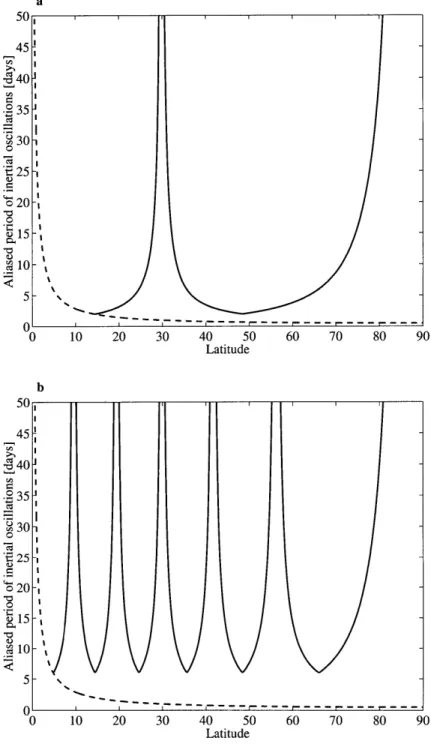
In POCM, prognostic fields are saved to storage every 3 model days, whereas the inertial period varies with latitude from 1/2 a day at the poles to infinitely long at the equator. Therefore, the saved model record only resolves the inertial oscillations where their period is greater than 6 days corresponding to within about 5Yof the equator. At higher latitudes where the sampling does not resolve the inertial oscillations, they are aliased in time, so that they impersonate oscillations with much longer periods. The aliasing frequencies follow from:

w =

f

At

with At = 3 day sampling period, and n = 0, 1, 2,... such that |wl < r/At. Because

150- 4100- 50--60 -40 -20 0 20 40 60 Latitude b 250 200- 150- 100-50 0 -60 -40 -20 0 20 40 60 Latitude

Figure 2.2: EKE along 200'E for forcing with (a) once per 3 days uninterpolated wind stress (thin solid line) and with once per 3 days linearly interpolated forcing (dashed line)

and (b) once per day linearly interpolated forcing (heavy solid line). EKE is in cm2 s--in Fig. 2.3 is the true period of s--inertial oscillations and their aliased period as a function of latitude for sampling periods (At) of once per day and once per 3 days. The latitudes at which the aliased period of the inertial motions go to infinity (the frequency, w = 0) follow from (2.8), substituting

At

It is impossible to eliminate aliasing due to the subsampling of the model; however, one can reduce the amplitude of the aliased inertial oscillation signal in the true EKE by saving filtered estimates of the prognostic variables instead of using instantaneous dumps of the variables every three days. An ideal filtering scheme would remove from

Latitude

0 10 20 30 40 50 60 70 80 90

Latitude

Figure 2.3: The true period of inertial oscillations (dashed) and their aliased period (solid) as a function latitude for sampling at (a) once per day and (b) once per 3 days.

the output all oscillations at frequencies higher than the Nyquist frequency of the output data. However, such filtering schemes would require knowledge of the entire

time history of the model to make a filtered estimate at any given time point, which is not realistic in an OGCM because of memory and/or disk storage requirements. But filters can be applied to the model during the run which only require knowledge from single timesteps over the output period. There is an extensive literature on the design and use of filters (Priestley 1981). Among the host of possible choices, the running average (or boxcar filter) and Hamming filter are commonly used and easy to implement. Note that a low pass filter (> 9 days) applied to the POCM 4_3 output will remove much of the spurious eddy energy associated with the inertial motions, but not where it was aliased into the mean fields.

2.3.1

Average fields

The running average requires only summing the variables in time over a given period and dividing by the number of time points included in the sum. If the period is chosen to be significantly greater than the period of the inertial oscillations, inertial energy will be removed from the output. A comparison of the zonally averaged EKE as a function of latitude for the original run with the result of tests 2 and 3 averaged over 3 day periods is shown in Fig. 2.4. The dominant feature to recognize is the removal of the large peaks in the EKE associated with the inclusion of the inertial oscillations in lower-frequency time-dependent motions. In the thin bands of low EKE in the

unfiltered estimate near 9.6', 19.40, 29.90, 41.70 and 56.20, the inertial oscillations

do not contribute to the EKE, since their aliased period is very long. In the filtered estimate, however, the inertial oscillations are removed from the output before the EKE calculation. Therefore, at these latitudes there is very little difference between the filtered and unfiltered estimates of EKE. The minor differences between tests 2 and 3 are real effects of the higher-frequency forcing used in test 3.

2.3.2

Hamming filter

The boxcar filter is the simplest filter to implement, requiring only that the model save the mean of the prognostic variables every three days. However, unless the length of the boxcar filter is much greater than the period of the oscillations which are to be

0 Latitude

Figure 2.4: (a) Zonal average EKE for April 1993 for the original run which used once per 3 days uninterpolated forcing and once per 3 days instantaneous sampling (thin solid line), test 2 with used once per 3 days linearly interpolated forcing and 3 day averaged samples (dashed line) and test 3 with once per day linearly interpolated forcing and 3 day averaged samples (heavy solid line). EKE is in cm2 -2.

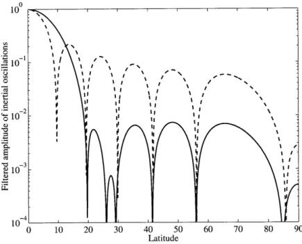
removed, or there is an integral number of complete oscillations within the period of the filtering, the boxcar filter can only weakly damp their amplitude because of the significant side lobes in the frequency domain of the boxcar filter. It is well known that tapering the sides of the filter in the time domain reduces the amplitude of the side lobes in the frequency domain. An excellent candidate for this application is the Hamming filter since it minimizes the side lobes in the frequency domain (Priestly 1981). The Hamming filter would be implemented in a similar fashion as the boxcar filter, except that, a weighting coefficient used for each time step is changed at each time step. The coefficients are given by the formula:

w (k) = 0.54 - 0.46 cos 2wk, 0 < k < n - 1, (2.10) (n - 1)

where n is the number of time steps in 3 days. We can compare the effectiveness of the boxcar and Hamming filters at damping an oscillation at the inertial frequency as a function of latitude. Figure 2.5 shows the damping coefficient of the filtered inertial oscillation as a function of latitude for the boxcar and Hamming filters. For a sampling period of 3 days, the filtered inertial energy poleward of ±19' is less than 1% of its original magnitude, whereas over a similar range, the boxcar filter is about an order of magnitude less effective.

Eddy Kinetic Energy

-

No averaging

45 90 135 180 225 270 315 360

Longitude

Eddy Kinetic Energy

-

3 day averages

45 90 135 180 225 270 315 360

Longitude

50 100

Eddy Kinetic Energy [cm2 s]-2

150

Figure 2.4: cont. (b) EKE calculated over 6 months from March through August 1993 for the original run (upper panel) showing aliased inertial oscillations and test 3 (lower panel) where the inertial oscillations have been removed by a 3-day boxcar filter.

-30 -60 60 30 0 -30 -60

10 -I If - IIf i~ If -2 \I 10 "CI -3 10 0-4 0 10 20 30 40 50 60 70 80 90 Latitude

Figure 2.5: Damping response coefficient for inertial oscillations as a function of latitude for a Hamming filter (solid line) and a boxcar filter (dashed line).

The inertial oscillations present in the model affect not only the velocity fields and eddy kinetic energy, but also higher-order products. The meridional heat transport is very sensitive to the aliasing induced by the inertial oscillations because in the model they carry a large amount of heat in the surface layer. It has a very large amplitude oscillation at the inertial frequency as can be seen in Fig. 2.6a. The heat transport across 25'N in the Atlantic Ocean calculated from hourly output from test case 1 shows an oscillation at the inertial frequency with an amplitude of about 1 Petawatt. Overlaying an arbitrary 3-day subsampling on it clearly gives a much different picture from what the full time series shows from hourly sampling. In Fig. 2.6b, the response in the zonal heat transport at 25'N with the boxcar filter is compared to that derived from a Hamming filter with a width of 3 days. The Hamming filter (solid line) damps out the inertial oscillations much more effectively than the boxcar filter (dashed line). From these considerations, it appears that the Hamming filter is the most appropriate to use to remove the inertial oscillations from the model records.

10 15 Model time [days]

Figure 2.6: (a) Unfiltered heat transport time series at 25'N in the Atlantic with the dots representing arbitrary once-per-3-days sampling. (b) Same results but using a 3-day running boxcar filter (thin solid line) and a 3 day running Hamming filter (heavy solid line) on the heat transport data.

2.4

Conclusions

This chapter has discussed how high-frequency forcing and associated sampling in models introduces aliased signals due to inertial oscillations into the sampled prog-nostic fields. It has been shown that inertial motions are aliased into longer-period motions whose frequency depends on the latitude and sampling rate. At some com-binations of latitude and subsampling period, the inertial motions can be aliased into the mean fields. The method used to perform the temporal interpolation of the wind stress fields can cause the high-frequency power spectrum to be distorted. For an investigator wishing to study high-frequency motions, such as inertial oscillations, these arguments indicate that it would be best to examine the model state at a very high frequency and force the model with high-frequency fields. However, for an inves-tigator studying the general circulation of the ocean, we recommend that some type of filtering prior to saving fields for later analysis be incorporated in the model run to remove the inertial oscillations. We also suggest that even when new forcing fields are read in every day, they need to be interpolated to every time step to remove steps in the forcing of the model.

2.5

Appendix: Derivation of interpolation spectra

The power spectra for the interpolation functions used in this chapter require some derivation. In order to have a framework in which to discuss them, the following indices are defined according to the following time line:

i=0 i=1 i=2 i=3

j=1 j=3 j=5 j=7 j=1 j=3 j=5 j=7 j=1 j=3 j=5 j=7 j=0 j=2 j=4 j=6 j=0 j=2 j=4 j=6 j=0 j=2 j=4 j=6 j=0 where i = 0, 1, 2, 3 ... are the time points where the data are provided, namely once every 3 days in this case, and

j

j = 0, 1, 2,

3 ... 143 if one is interpolating the once per day wind fields. (If one is interpolating

the once per day winds fields then

j

In the original method of using the wind stress without any interpolation:

rf = ai (2.11)

for all

j,

If the ai are uncorrelated, so that: (akal) - 6k,I, where 6k,I is the Kronecker delta

function, then the autocorrelation function for this interpolant is:

1 0< <h

h - -<T

p(T) = (2.12)

0 T> h

where p is the correlation coefficient, T is the time lag and h is the time between the original data points. It is an even function, so negative time lags are equivalent to positive time lags. Assuming the original data have a standard deviation of 1, then

No interpolation 2 1.5-0.5- a c 0~ c -0.5--1 -1.5--2 1 2 3 4 5 6 7 8 9

Figure 2.7: No interpolation between data points

the interpolated function also has a standard deviation of 1 (given by the square-root of the zero lag of the auto-correlation function). The Fourier transform of the auto-correlation function gives the power spectrum:

S (W) 02[1 - cos (wh)] =sine2 _{(wh) (2.13)}

(wh)2 2

This power spectrum falls off like w-2, but it has zero variance lines every wh = n7r,

n = 1, 2, 3, ... which can cause undesirable depleted energy bands.

Following the same notation, the linear interpolation method would be denoted:

T = ai + bi(jAt) (2.14)

where bi = (ai+1 - ai)/h, where ai is again the wind stress read in from the data

files for that day, and ai+1 is the wind stress for the next day and h = 3 days (for the case of interpolating 3 day averaged winds). Using this method the interpolated function is now continuous in time, but its first derivative has offsets between at the data points. Figure 2.8 illustrates this method.

Linear interpolation 2A 1.50.5 - -0.5--1.5 -1 2 3 4 5 6 7 8 9

Figure 2.8: Linear interpolation between data points

73 T2 2

2h3 h2 ₃

pT 3 T2 27 4 (2.15)

6h3 h2 _{h 3}

0 T>2h.

Again it is an even function and assuming the original data have a standard deviation of 1, then the interpolated function has a standard deviation of y/2/3 ~ 0.816. So the interpolated function has 82% of the total variance of the original data. This issue and methods to alleviate it were addressed by Killworth (1996). The power spectrum is:

S

(wh)4 2

What has been gained using this method is that the power spectrum at high frequen-cies falls off much faster, like w-4, and the number and position of the zero energy bands have not changed.

Still using two data points ai and ai+1 one can write the following interpolation method using a cosine function:

, a. - ai+1 aj a,

+

r. = Cos + (2.17)

2 h 2