Dynamic stiffness and transfer matrix analysis of marine riser vibration

(1)

Dynamic Stiffness and Transfer Matrix Analysis of Marine

Riser Vibration

by

Yongming Cheng

Submitted to the Department of Ocean Engineering

in partial fulfillment of the requirements for the degree of

Doctor of Philosophy

at the

MASSACHUSETTS INSTITUTE OF TECHNOLOGY

January 2001

Dfe-b( 200j

@

Yongming Cheng, MMI. All rights reserved.

The author hereby grants to MIT permission to reproduce and

distribute publicly paper and electronic copies of this thesis document

in whole or in part.

Signature Redacted

Author...

Department of Ocean Engineering

January 24, 2001

Signature Redacted

C ertified by

...

..

...

J. Kim Vandiver

Professor of Ocean Engineering

Thesis Supervisor

Signature Redacted

Accepted by... ...- -..-. ...

Nicholas Patrikalakis

MASSACHUSETTS INSTITUTE

Kawasaki Professor of Engineering

OF TECHNOLOGY

_Chairman,

_{partment Committee on Graduate Students}

APR 18 2001]

AFC

(2)

Dynamic Stiffness and Transfer Matrix Analysis of Marine

Riser Vibration

by

Yongming Cheng

Submitted to the Department of Ocean Engineering on January 24, 2001, in partial fulfillment of the

requirements for the degree of Doctor of Philosophy

Abstract

This dissertation extends the use of the dynamic stiffness and transfer matrix methods in marine riser vibration. Marine risers possess a predominant chain topology. The transfer matrix method is appropriate for the analysis of such structures. Wave trans-mission and reflection matrices are formulated in terms of transfer-matrix elements. The delta-matrix method is introduced to deal with numerical problems associated with Yery long beams and high frequencies. The general internal relationships be-tween the transfer matrix and dynamic stiffness methods are derived and applied to the problem of a non-uniform beam with discontinuities. An implicit transfer matrix of a general non-uniform beam is derived.

The vibration analysis of non-uniform marine risers is addressed by combining the procedure of the dynamic stiffness method with the WKB theory. The WKB-based dynamic stiffness matrix is derived and the frequency-dependent shape function is expressed implicitly. The Wittrick-Williams algorithm is extended to the analysis of a general non-uniform marine riser, allowing automatic computation of natural frequencies. Marine riser models with complex boundary conditions are analyzed. The WKB-based dynamic stiffness method is improved and applied to a non-uniform beam system with discontinuities. A dynamic stiffness library is created.

Dynamic vibration absorbers and wave-absorbing terminations are investigated as a means of suppressing vibration. The optimal tuning of multiple absorbers to a non-uniform beam system under varying tension is investigated. The properties of wave-absorbing terminations of a beam system are derived.

The vibration of two concentric cylinders coupled by the annulus fluid and by periodic centralizers is modeled. The effects of coupling factors on vibration are nu-merically evaluated. It is shown that a properly designed inner tubular member may be used to damp the flow-induced vibration of the outer cylinder.

(3)

Acknowledgments

First and foremost, I would like to express my deep gratitude to my supervisor, Pro-fessor J. Kim Vandiver, for his guidance and support through this research. I enjoyed our weekly meetings. His clear thinking, strong engineering sense, and rich research experience got me through the tough times. His creative work in vortex-induced vi-bration is well known. From him I learned how to approach a complex problem and find solutions to satisfy an engineering requirement. His endless understanding, kind encouragement and great assistance will always be appreciated.

I am also indebted to the other members of my thesis committee, Professor

Ed-uardo Kausel, Professor Jerome H. Milgram, Professor Geir Moe (NTNU, Norway), and Dr. Leonard Imas for their time and suggestions.

I would like to thank the members of the industry consortium who supported this

thesis work: Aker, BP/Amoco, Chevron, Exxon/Mobil, Petrobras, Shell, Statoil, and Texaco.

I would like to thank all members of our research group for fruitful discussions on

various projects. I enjoyed our weekly group meetings.

Thanks to Mrs. Shiela McNary for her administrative assistance and the MIT writing Center for editing the draft of this thesis.

Thanks to my parents and in-law for their support and encouragement. Thanks to my son, Bohao Cheng. He helped me to forget difficulties and took me into his world. I enjoyed our discussion about how to prevent whales and sharks from eating risers. It was a big fun to play with him. Thanks to my wife, Haiyan Li. She kept me grounded through all the ups and downs. She took such good care of Bohao and me. I dedicate this thesis to her with all my love.

(4)

List of Figures

2-1 A typical uniform beam section . . . . 27

2-2 A beam divided into n sections . . . . 28

2-3 The determinant of the transfer matrix versus frequency . . . . 33

2-4 The simply-supported constantly tensioned uniform beam attached by a mass-spring absorber at the midpoint . . . . 34

2-5 _{The determinant of the transfer matrix versus frequency . . . .} 35

2-6 The first four modes of the composite system . . . . 36

2-7 The transfer mobility of the free-free pipe . . . . 37

2-8 The simply-supported constantly tensioned uniform beam attached by a mass-spring absorber at the midpoint . . . . 37

2-9 The transfer mobility of the free-free pipe with mass attachment . . . 38

2-10 The modulus of transmission coefficients . . . . 44

2-11 The reflection and transmission coefficients of r and t . . . . 45

2-12 The determinant versus frequency (Hz) . . . . 50

2-13 The determinant versus frequency (Hz) . . . . 51

2-14 The delta-matrix determinant versus frequency (Hz) . . . . 53

2-15 The approximation scheme (a) . . . . 54

2-16 The approximation scheme (b) . . . . 54

2-17 The approximation scheme (c) . . . . 55

2-18 The absolute determinant of the riser versus frequency in Hz ( approx-im ate schem e (a) ) . . . . 56

2-19 The absolute determinant of the riser versus frequency in Hz ( approx-im ate scheme (b) ) . . . . 56

(10)

2-20 The absolute determinant of the riser versus frequency in Hz

(approx-im ate schem e (c) ) . . . . 57

2-21 The absolute determinant of the riser versus frequency in Hz (approx-im ate schem e (a) ) . . . . 58

2-22 The absolute determinant of the riser versus frequency in Hz (approx-im ate schem e (b) ) . . . . 58

2-23 The absolute determinant of the system versus frequency in Hz . . . . 64

3-1 The determinant of the dynamic stiffness matrix versus frequency . . 75

4-1 The determinant of the dynamic stiffness matrix of a 500-ft riser versus frequency . . . . 87

4-2 The first three natural mode shapes for a 500-ft riser . . . . 88

4-3 The mass density variation of the Helland riser . . . . 90

4-4 The tension variation of the Helland riser . . . . 91

4-5 The comparison of the natural frequencies with those obtained by Shear7 91 4-6 The 20th mode shape of the Helland riser . . . . 92

5-1 The comparison of the natural frequencies with those obtained by Shear7 99 5-2 The 1st mode shape, slope and curvature of the 1400-ft riser ... 103

5-3 The 2nd mode shape, slope and curvature of the 1400-ft riser ... 104

5-4 The 3rd mode shape, slope and curvature of the 1400-ft riser . . . 104

5-5 The 4th mode shape, slope and curvature of the 1400-ft riser . . . 105

5-6 _{The 5th mode shape, slope and curvature of the 1400-ft riser . . . 105}

5-7 The 6th mode shape, slope and curvature of the 1400-ft riser . . . 106

5-8 _{The 7th mode shape, slope and curvature of the 1400-ft riser . . . 106}

5-9 The 13th mode shape, slope and curvature of the 1400-ft riser . . . . 107

5-10 The 1st mode shape, slope and curvature of the Helland riser . . . 108

5-11 The 2nd mode shape, slope and curvature of the Helland riser . . . . 108

(11)

5-14 The 5th mode shape, slope and curvature of the Helland riser . . . . 110

5-15 The 18th mode shape, slope and curvature of the Helland riser . . . . 110

5-16 The 20th mode shape, slope and curvature of the Helland riser . . . . 111

5-17 The determinant of the fixed-fixed 1400-ft riser versus frequency . . . 112

5-18 The determinant of the fixed-fixed 400-ft riser versus frequency . . . . 113

5-19 The absolute determinant (loglO) of the fixed-fixed 400-ft riser versus frequency ... ... 113

5-20 The 1st mode shape, slope and curvature of the free-pinned beam with varying tension . . . . 115

5-21 The 5th mode shape, slope and curvature of the free-pinned beam with varying tension . . . . 115

5-22 The 1st mode shape, slope and curvature of the 1400-ft riser with rotational springs . . . . 117

5-23 The 5th mode shape, slope and curvature of the 1400-ft riser with rotational springs . . . . 117

5-24 The 1st mode shape, slope and curvature of the free-pinned beam with varying tension and rotational spring at x = 1 . . . . 118

5-25 The 5th mode shape, slope and curvature of the free-pinned beam with varying tension and rotational spring at x = 1 . . . . 119

6-1 A member with section changes . . . 124

6-2 Frequency analysis of the 1400-ft riser using a new type of delta-matrix 130 6-3 Frequency analysis of the 1400-ft riser by 3 and 10 elements respectively130 6-4 A submerged floating pipeline . . . . 131

6-5 A beam system with absorbers . . . 132

6-6 The determinant of the system versus frequency . . . 132

7-1 Beam with a damped dynamic vibration absorber . . . 138

7-2 Finding roots of p2 _ f2 _ If 2p2H(h, h) = 0 for p = A₁ . . . . 144

7-3 The relationship between p and

f

(p = 1/5) . . . . 146

(12)

7-5 The frequency response curves (p = 1/5, p = 0.6) . . . . 147

7-6 The frequency response curves (p = 1/5, po = 0.56) . . . . 148

7-7 The frequency response curves (p = 1/5, po = 0.56) . . . . 148

7-8 Comparison of response curves with different tuning (p = 1/5) . . . . 149

7-9 Frequency response of a simply supported beam with 1st natural fre-quency tuned by one DVA (M = 1/5) . . . . 155

7-10 Frequency response of a simply supported beam with the 1st natural frequency tuned by one and two DVAs respectively . . . . 155

7-11 Frequency response of a simply supported beam with the 3rd natural frequency tuned by multiple DVAs . . . . 156

7-12 Frequency response of a uniform riser with its 1st frequency tuned by m ultiple DVAs . . . . 161

7-13 Frequency response of a non-uniform riser with its 1st natural fre-quency tuned by multiple DVAs . . . . 162

7-14 Frequency response of a non-uniform riser with its 6th natural fre-quency tuned by seven DVAs . . . 162

7-15 Frequency response of a damped non-uniform riser with its 3rd natural frequency tuned by three DVAs . . . 163

7-16 A wave absorbing termination . . . 164

7-17 Wave reflection coefficient at the termination . . . 169

8-1 _{A double-beam system coupled by springs and dampers . . . 172}

8-2 _{Two-degrees-of-freedom system for nth mode . . . 176}

8-3 Effects of spring stiffness on synchronous and asynchronous natural frequencies . . . 179

8-4 Frequency response of the 15th mode due to a concentrated force 180

8-5 Frequency response of the 15th mode due to a concentrated force 184

8-6 The first four synchronous and asynchronous mode shapes (Case 1) 188

(13)

8-8 First four synchronous and asynchronous mode shapes by the

WKB-DSSM (solid line: Beam 1; dash-dot line: Beam 2) . . . . 192

8-9 First four synchronous and asynchronous mode shapes by using closed

form solutions (solid line: Beam 1; dash-dot line: Beam 2) . . . . 193

8-10 The third in-phase mode shapes(rs, = 10, solid line: Beam 1; dash-dot

line: Beam 2) . . . . 194

8-11 Schematic of two concentric tubes containing a viscous fluid . . . 195

8-12 The first 8 mode shapes of the coupled system (k* = 1/48, solid line:

external riser; dash-dot line: internal riser) . . . 208

8-13 The 9th to 16th mode shapes of the coupled system (k* = 1/48, coupled

by the fluid and springs) . . . 209

8-14 The first 8 mode shapes of the coupled system (k* = 1, solid line:

8-15 The 9th to 16th mode shapes of the coupled system (k* = 1, coupled

by the fluid and springs) . . . 212

8-16 The first 8 mode shapes of the coupled system (k* = 1000, solid line:

8-17 The 9th to 16th mode shapes of the coupled system (k* = 1000, coupled

by the fluid and springs . . . 214 8-18 The RMS frequency response of the external riser (fluid coupled, NCOUP=2) 218 8-19 The RMS frequency response of the internal riser (fluid coupled, NCOUP=2) 219 8-20 The RMS frequency response of the external riser (fluid coupled, NCOUP=2) 220 8-21 The RMS frequency response of the internal riser (fluid coupled, NCOUP=2)221 8-22 The RMS frequency response of the external riser (generally coupled,

NCOUP=3) . . . 223 8-23 The RMS frequency response of the internal riser (generally coupled,

NCOUP=3) . . . .

...224

8-24 The RMS frequency response of the external riser (generally coupled,

(14)

8-25 The RMS frequency response of the internal riser NCOUP=3) . . . . 8-26 The RMS frequency response of the external riser NCOUP=3) . . . . 8-27 The RMS frequency response of the internal riser NCOUP=3) . . . . 8-28 The RMS frequency response of the external riser

NCOUP=3) . . . . 8-29 The RMS frequency response of the internal riser NCOUP=3) . . . . 8-30 The RMS frequency response of the external riser NCOUP=3) . . . . 8-31 The RMS frequency response of the external riser

NCOUP=3).... ... (generally coupled, .(.g. . . . . (generally coupled, .(.. . . . . (generally coupled, .(.g. . . . . (generally coupled, (generally coupled, (generally coupled, . . . . (generally coupled,

A-1 Natural frequencies of the 1400-ft riser . . . . A-2 The first three mode shapes of the 1400-ft riser . . . . C-1 Combination of beam with point mass . . . . C-2 Combination of tensioned beam with point mass . . . . C-3 Combination of tensioned beam with spring-dashpot support .

C-4 Combination of tensioned beam with an absorber . . . .

C-5 Combination of tensioned beam with concentrated mass and

inertia . . . .. . . .

C-6 Combination of tensioned beam with concentrated mass and

support ... ... D-1 D-2 D-3 . . . . 256 9;8 rotary spring

The displacement along the riser . . . . The acceleration along the riser . . . . The acceleration along the riser . . . .

226 228 229 230 231 233 234 242 243 253 254 259 261 265 266 266

(15)

List of Tables

2.1 Comparison of natural frequencies found by using the TMM and the

analytical solutions . . . . 33

2.2 Delta-matrix lexicon . . . . 47

2.3 Comparison of natural frequencies (Hz) found by using the delta-matrix and the analytical solutions . . . . 51

2.4 Comparison of natural frequencies (Hz) found by using the delta-matrix and Shear7 . . . . 52

2.5 Natural frequencies (Hz) of the composite system . . . . 64

3.1 Complex natural frequencies of a damped beam . . . . 78

4.1 Comparison of circular natural frequencies . . . . 88

5.1 Comparison of natural frequencies (Hz) . . . . 98

5.2 Natural frequencies (Hz) of the 1400-ft riser under different spring stiff-ness ratios . . . . 116

7.1 Frequencies of a cantilever beam with an undamped DVA (b = 1/2, h = l,, = 1/5) . . . . 145

8.1 Comparison of natural frequencies fi (Hz) of synchronous vibrations 178

8.2 Comparison of natural frequencies f2n (Hz) of asynchronous vibrations 178

8.3 Comparison of natural frequencies

fr,,

(Hz) of synchronous vibrations 183

(16)

8.5 Comparison of natural frequencies(Hz) of asynchronous and synchronous

vibrations (Case 1) . . . . 187

8.6 Comparison of natural frequencies(Hz) of asynchronous and synchronous vibrations (Case 2) . . . 189

8.7 Comparison of natural frequencies fi (Hz) . . . . 191

8.8 Comparison of natural frequencies f2n (Hz) . . . . 191

8.9 Coefficients of natural mode shapes ai,(rs8 = 1.0) . . . . 193

8.10 Coefficients of natural mode shapes ain (rsp = 10) . . . . 194

8.11 Natural frequencies (Hz) of the double-riser system coupled by only springs . . . 206

8.12 Natural frequencies (Hz) of a coupled two-riser system . . . 207

8.13 Natural frequencies (Hz) of a coupled two-riser system . . . 210

8.14 Complex circular frequencies(w = Wr + iwj) of a coupled two-riser sys-tem . . . .. . ...215

A.1 Comparison of natural frequencies (Hz) . . . 243

A.2 Comparison of natural frequencies (Hz) . . . 244

(17)

Chapter 1 Introduction

1.1 Problem Statement

Marine structures such as production risers and deep-water pipelines are susceptible to Vortex-Induced Vibration (VIV), which results from complicated, non-linear in-teractions between structural motions and vortex-shedding. VIV is of great practical importance because it may cause fatigue failure.

Much research has focused on understanding the VIV phenomenon. King (1977) [2], Sarpakaya (1979) [3], and Griffin and Ramberg [4] reviewed the early studies of VIV and its applications. Vandiver (1993) [5] summarized his 17 years of experimen-tal observations, discussed the phenomenon of long flexible cylinders, and identified the dimensionless parameters important to the prediction of VIV. Recently, Vandiver, Allen, and Li (1996) [6] investigated the occurrence of lock-in under highly sheared conditions and indicated two dimensionless parameters to predict the likelihood of the occurrence.

There is broad research work done on structural dynamic analysis and on the VIV suppression of marine risers. Kim (1983) [7] assumed that the continuous coefficients are slowly varying and used the WKB asymptotic method to analyze a slender beam. The MIT Sea Grant Program supported the studies on the dynamics of compliant risers and cable dynamics, shown respectively in the references by Patrikalakis, et al

(18)

used the transfer matrix method to study the dynamics of strings with rigid lumps, and evaluated their effects on wave propagation. Vandiver and Li (1994) [12] devel-oped for tension-dominated structures a device called a wave absorbing termination, which is capable of suppressing the vibration. Levesque (1997) [13] studied vibration suppression in a finite length string with constant tension using the transfer matrix method and found that a translational mass-spring-dashpot absorber works better than in-line absorbers.

There are a number of analysis programs [17], such as SHEAR7, VIVA, and

Vi-CoMo, available to the industry to predict the VIV of marine risers. SHEAR7, which

is widely applied, uses mode superposition of uniform string and beam models to eval-uate which modes are likely to be excited, and estimates the cross-flow VIV response in steady, uniform or shear flows. The program is capable of evaluating multi-mode, non-lock-in response, as well as single-mode, lock-in response.

As offshore drilling and production proceed into deep waters, marine risers become longer and more flexible. Deepwater marine risers are very susceptible to VIV [18]. The increase in length lowers the natural frequencies and the magnitude of current required to excite the VIV. Long slender risers with complicated boundary condi-tions can cause numerical difficulties in dynamic analysis. A typical marine riser is a long non-uniform beam structure with discontinuities. Its variable properties include mass density, bending stiffness, and effective tension. Due to discontinuities such as buoyancy elements, the mass per unit length changes discontinuously. The dynamic behavior of such a slender system having variable properties and discontinuities is difficult to predict.

Floating production platforms require more complex riser configurations for well production or fluid injection fluids, between the subsea well-heads and the surface production facilities [19]. One type of riser assembly is made up of two concentric cylinders separated by a gap filled with viscous fluid. Centralizers are discretely and longitudinally distributed in between the two cylinders. Both predicting VIV and

(19)

This thesis focuses on the dynamics of a long slender non-uniform riser structure and a coupled double-riser system. The specific objectives are as follows:

(1) to construct effective numerical approaches for a long non-uniform marine

riser with discontinuities and variable properties including bending rigidity, mass per unit length, and effective tension;

(2) to explore new means such as dynamic vibration absorbers and wave-absorbing terminations to control vibration; and

(3) to formulate a coupled double-riser system and to numerically evaluate the

effects of coupling factors, such as fluid viscosity and spacing of centralizers between two risers.

1.2 Technical Summary of Numerical Methods

A typical marine riser is a non-uniform beam structure with discontinuities. An

an-alytical solution to its partial differential equation is generally not possible. We have to use a numerical technique for analyzing the dynamic behavior of a marine riser. A number of approaches can be employed to analyze marine risers, such as the Transfer Matrix Method (TMM), the Finite Element Method (FEM), the Finite Difference Method (FDM), and the Dynamic Stiffness Method (DSM). Each method has its advantages and disadvantages.

The transfer matrix method

The TMM, also known as the line-solution technique, has its origin in Germany. It is one of the most appropriate methods for the analysis of a chain-type structure because only successive multiplications are necessary to fit the elements together and intermediate conditions have no effect on the order of transfer matrix required. Hence, this method handles discontinuities very conveniently.

The line-solution methodology theoretically can be applied to appropriate struc-tural members to solve problems involving almost any physically conceivable situa-tions to which a line-type solution applies. However, the fact that a computer requires

(20)

calculations to be performed on the basis of a limited number of digits introduces com-plications into the numerical implementation of a line solution for certain classes of members, such as those members whose higher natural frequencies are to be sought and those members which include stiff spring supports. Numerical problems arise when large, almost equal numbers are subtracted. Due to the limited number of dig-its carried by computers, the results may be inaccurate or totally meaningless.

It has been found that the TMM works quite well for a string model but will have numerical problems for a beam structure when its length is larger and a high natural frequency analysis is desired. In this case, we have to improve the TMM to avoid the numerical problems.

The finite element method and the finite difference method

The FEM is a flexible and powerful tool which is widely used in engineering, and which in particular is employed extensively in the analysis of solids and structures. The FEM requires the division of a structural domain into many subdomains called elements. On the basis of frequency-independent shape functions, it effectively re-duces a continuous model into one having finite degrees of freedom. The accuracy with which the behavior of the substitute finite degrees-of-freedom system represents that of the real structure clearly depends on the number of elements and their as-sumed shape functions. The FDM gives a pointwise approximation of the governing equation. The accuracy of this method depends on the number of grid points. It can give accurate results if sufficient grid points are used. Hence, both methods are effective for the analysis of lower frequencies of structures. If high natural frequencies are to be sought, a large number of degrees of freedom is required.

For a uniform beam element under linearly varying tension, we have found the stiffness matrix using the FEM, shown in Appendix A. This matrix is more efficient than that of a conventional constantly-tensioned element in analyzing a uniform riser under linearly varying tension.

(21)

since it is based on the exact dynamic stiffness matrix derived from the free vibration analysis. The DSM performs free and forced vibration analysis within the differential equation theory of beams, thus avoiding assumed modes and lumped masses. This method enables one to analyze an infinite number of natural frequencies and modes

by means of a finite number of degrees of freedom. The difference between the DSM

and the FEM is that the shape function in DSM is frequency-dependent while that in the FEM is independent of frequency. The DSM is appropriate for the analysis of low frequencies as well as high frequencies.

A marine riser structure possesses a predominant chain-type topology. For

ris-ers in deep water areas, the high order natural frequencies and multiple modes are potentially excited by VIV. Hence, this thesis employs and explores the TMM and

DSM for the analysis of a long slender non-uniform riser structure and a complicated

coupled double-riser system.

1.3 Overview of this thesis

This thesis investigates the vibration analyses of a long slender non-uniform riser structure with discontinuities and a coupled double-riser system by improving the transfer matrix and dynamic stiffness methods, explores new means such as dynamic vibration absorbers and wave-absorbing terminations to control vibration, and eval-uates the effects of coupling factors on the frequency response of a coupled dual riser system.

Chapter 1 states the topic and specific objectives of this thesis, summarizes the numerical methods which are employed for the analysis of marine risers, and presents the two methods, the TMM and DSM, to be used and explored in the thesis.

Chapter 2 discusses the transfer matrix method and its application for a beam structure. The first few sections outline the transfer matrix method and illustrate the applications with examples. In order to consider wave propagation in a beam structure with discontinuities, the chapter derives wave transmission and reflection

(22)

matrices in terms of transfer-matrix elements. The method presents numerical prob-lems in analyzing a beam structure when the length is very large or high natural frequencies are desired. The chapter specifically introduces the delta-matrix method and illustrates the method with examples. We often approximate a non-uniform beam

by a number of stepped uniform ones. This chapter investigates three approximate

schemes for a beam structure under variable tension and shows their convergence rates with an example. This chapter finally presents a symbolic operation-based transfer matrix method to avoid numerical problems.

Chapter 3 introduces the dynamic stiffness matrix analysis of a uniform beam structure and discusses the analysis of complex natural frequencies. For a uniform Euler beam, the chapter derives the elemental dynamic stiffness matrix and the cor-responding frequency-dependent mass and stiffness matrices. The global dynamic stiffness matrix is then assembled as in the FEM. Natural frequencies are determined

by equating the frequency determinant to zero. The chapter introduces the

Wittrick-Williams (W-W) algorithm, as a more reliable method for determining natural fre-quencies. In order to include damping effects, this chapter finds complex frequencies

by means of the Muller method.

Chapter 4 investigates the vibration analysis of non-uniform marine risers by com-bining the DSM procedure in Chapter 3 with the WKB theory, which assumes that the coefficients in the differential equation of motion are slowly varying. The WKB-based elemental dynamic stiffness matrix is first derived and the frequency-dependent shape function is expressed implicitly. Natural frequencies are found by equating to zero the determinant of a global dynamic stiffness matrix. Two non-uniform risers appear as an illustration of the efficiency of this method.

Chapter 5 extends the W-W algorithm to the analysis of a general non-uniform marine riser and combines the algorithm with the WKB-based dynamic stiffness method described in Chapter 4. This technique allows automatic computation of natural frequencies of a non-uniform beam structure. On the basis of the

(23)

WKB-ary conditions.

Chapter 6 generalizes the internal relationship between the TMM and the DSM and discusses its application. Due to different sign conventions which may be used in the two methods, the chapter generalizes the relationship by introducing correspond-ing transformation matrices. Uscorrespond-ing this internal relationship, the chapter then derives an implicit transfer matrix of a non-uniform beam from the dynamic stiffness matrix found in Chapter 4 and shows the application by an example of a riser under linearly varying tension. Again, using the relationship, the chapter improves the WKB-based

DSM for describing a non-uniform beam structure with discontinuities. Further using

the relationship, this chapter establishes a dynamic stiffness library.

Chapter 7 discusses the vibration suppression of a general beam structure by means of dynamic vibration absorbers and wave-absorbing terminations. The first few sections introduce the optimal tuning of a single dynamic vibration absorber to a uniform beam. The chapter next studies optimal tuning of multiple identical dynamic absorbers to a uniform beam with general boundary conditions. The chapter next investigates optimal tuning of multiple identical absorbers to a non-uniform beam system under varying tension. Since practical structures have structural damping, the chapter discusses the effects of structural damping on the optimal tuning. Based on the research by Vandiver and Li, this chapter further extends the analysis of wave-absorbing terminations of a beam system.

Chapter 8 systematically investigates the vibration analysis of coupled beams. The first few sections discuss the coupled vibration analysis and the optimal tuning of a dynamic absorbing beam, coupled by distributed springs and dampers to a second beam. The chapter then analyzes the coupled system in which both uniform beams are under constant tension. The complexity of the coupled system is next increased

by the introduction of an ideal fluid in between two beams. The effects of the fluid on

natural frequencies and mode shapes are discussed. A practical composite riser struc-ture is modeled as a generally coupled double-beam system, in which both beams are non-uniform ones under variable tension, the fluid in between the beams is viscous, and stiffness and damping from discrete centralizers are longitudinally distributed.

(24)

The chapter mathematically formulates the coupled system, numerically solves for both real and complex natural frequencies, and evaluates the effects of coupling fac-tors on the vibration.

Chapter 9 summarizes new contributions made in this thesis and recommends further research in the future.

(25)

Chapter 2 Transfer Matrix Method

2.1 Introduction

The transfer matrix method is ideally suited to vibration analysis of a structure which has a predominant chain topology. The size of the transfer matrices is dependent on the order of the differential equations of the system. Discontinuities such as a con-centrated mass and a mass-spring absorber present no difficulty since they have no effect on the order of the transfer matrices required. A marine riser is a chain-like structure and it is convenient to employ the transfer matrix method to analyze it. Li and Vandiver [11, 20] modeled a marine riser as a string system and studied the wave propagation by the transfer matrix method.

However, this method has numerical problems in solving beam-like structures when the structural length is very large or high order natural frequencies are desired [21]. Researchers have been improving the method to avoid the numerical problems [22].

The next section of this chapter briefly outlines the transfer matrix method. The third section illustrates the applications of the method with examples, solving for nat-ural frequencies and mode shapes. The fourth section derives the wave transmission and reflection matrices in a beam structure due to discontinuities and gives illus-trative examples. The fifth section discusses the numerical problems of the method in analyzing a beam structure, specifically introduces the delta-matrix method, and

(26)

illustrates the improved method with examples. The sixth section investigates three approximate schemes for a beam structure under variable tension and shows their con-vergence rates with an example. The final section of this chapter presents a symbolic operation-based transfer matrix method to avoid the numerical problems.

2.2 An outline of the transfer matrix method

2.2.1 state vector and transfer matrix

The state vector at a point i of an elastic system is a column vector whose components are the generalized displacements and the corresponding generalized forces at the point. For a uniform beam, the displacements are lateral displacement y and slope 6,

and the corresponding forces are shear force

Q

and bending moment M. The state

vector in this case is:

y 0

si _(2.1)

M

Q

We should note that the displacements and corresponding forces in Eq. (2.1) are in positions which are symmetrical about the center of the column.

We define the transfer matrix as the matrix which relates two state vectors at different positions in an elastic system, namely:

si+1 = Ui si, (2.2)

in which Uj is the transfer matrix and si and si+1 are the state vectors at stations

i and i + 1, respectively. It is evident that if there are n components in the column

vector, then the transfer matrix is square and of the order of n. When i and i + 1 are the different points of a continuous system, the transfer matrix relating the state

(27)

There are a number of approaches to deriving a field matrix [21]. A uniform beam section, shown in Figure 2-1, appears as an example.

R

I

i+1

x

Figure 2-1: A typical uniform beam section The differential equation of motion for a beam is:

d" Y

EIlz - pAw2Y =O, (2.3)

where pA is the mass per unit length, EI is the bending stiffness, and Y is the transverse displacement amplitude. We find its transfer matrix on the basis of Eq.

(2.3): S(klj) kV(ki) Elk2 U(klj) EIk3T(kj) Ek V(k1j) S(kj) EIkV(k2) Elk2_U(klj) ggT(kj) E1 U(klj) S(kli) kV(ki) -T(klj) S(klj) in which k4 = PAT2

and the frequency-dependent functions are:

EI S(kli) T(kli) U(kli) V(k4j) = [cosh(klj) + cos(k4j)]; 1 = [sinh(kl) + sin(k)]; 2 1 = [cosh(k) - cos(kli)]; 2 1 = [sinh(kl) - sin(kl)]. 2

A point matrix relating the left and right state vectors at a discontinuity can be

F

Ui = _, _(2.4) M QL 4+1 -1T(klj) 1 gU(klj)

(28)

constructed by considering dynamic equilibrium of the point.

2.2.2 Eliminating intermediate state vectors and finding

fre-quency determinant

Elimination of intermediate state vectors

Taking a uniform beam as an example, we divide the beam into n sections without lumping the masses at the station points, as shown in Figure 2-2.

I I I

0 12 j j+1 n-2 n-I n

Figure 2-2: A beam divided into n sections

Equation (2.4) shows the transfer matrix of a uniform beam. The following matrix relations exist between adjacent state vectors:

SL =U1so; = U2s; L Sn = _Un-isn-2;R = Us5_1. (2.5) Noting that s = s (i = 1, 2, equations in (2.5):

-.- _{n - 1) in this case, we obtain from the last two}

Sn = Un Un_1sn_ 2. (2.6)

We continue this procedure until obtaining the relation between the state vectors at the two ends of the beam:

(29)

where U is the overall transfer matrix formed by taking the products of all the inter-mediate transfer matrices in the order indicated. In this manner all the interinter-mediate state vectors have been eliminated.

Frequency determinant Equation (2.7) is expanded as:

y U1 1 U1 2 U1 3 U1 4 Y

0 U_{2 1} U2 2 U2 3 U2 4 0(28)

M U3 1 u32 U33 u3 4 M

Q

U41 U4 2 U43 U4 4

Q

-The frequency determinant is formulated by applying the boundary conditions to Eq.

(2.8). For a simply-supported beam, the boundary conditions are:

Yo = 0, Mo =, y = 0, Mn = 0. (2.9)

Substituting Eq. (2.9) into (2.8) leads to:

U1 2 0o + U14 Qo 0,

U₃2 00 + U34 Qo = 0. (2.10)

For a nontrivial solution of Eq. (2.10), the determinant of the coefficients must be zero, namely:

u12 U14 =

=1 0. (2.11)

U3 2 U3 4

Since the elements Uik, (i, k =1, ... , _{4) are known functions of the circular frequency}

w, _{this frequency determinant serves to calculate the natural frequencies of the beam}

structure.

For other boundary conditions the frequency equation will require that other sub-determinants of the overall transfer matrix U vanish. For example, for a beam clamped at station 0 and free at station n, we find the frequency equation by following

(30)

the same procedure:

U_{3 3} U3 4 0.

(2.12)

U4 3 U4 4

Once the natural frequencies are known, we set equal to one one of the state com-ponents corresponding to the final frequency determinant. The other state component is found by means of one of the final equations such as Eq. (2.10). It then follows that the corresponding state variables at all stations can be determined. Hence, we obtain the mode shape in this procedure.

2.2.3 Response analysis

In order to find steady-state forced vibrations, we add an extra column to the transfer matrix Eq. (2.4) to include forcing terms. The extended state vector and transfer matrix are: y 9i = M ,(2.13)

Q

1 U1 1 U12 U1 3 U14 0 U2 1 U2 2 U2 3 U2 4 0 U= U3 1 U3 2 U3 3 U3 4 fm , (2.14)

U41 U42 U43 U44 fq

0 0 0 0 1

where fm and fq are external moment and force, respectively.

(31)

harmonic force p(t) = poeiwt acts, is: 1 0 0 0 0 0 1 0 0 0 U= 0 0 1 0 0 . (2.15) w mi 0 0 1 Po 0 0 0 0 1

As in the undamped case, the relation between the state vectors at the boundaries

0 and n of the system is achieved by the multiplication of the extended transfer

matrices. The unknown initial parameters at the boundaries are first solved. Hence the state vector at each node can be obtained as previously.

2.3 Vibration analysis of a beam structure with

discontinuities

In order to solve natural frequencies and mode shapes, we first find field matrices of continuous sections and point matrices at discontinuities. For a uniform beam section under constant tension, we derive its transfer matrix from the differential equation of motion, as shown in the example of Section 2.7. The transfer matrix is also available in [21]. However, we need to note the differences in the sign convention. The point matrix describing the mass-spring-dashpot absorber is found as follows:

1 0 0 0 0 1 0 0 Uc = (2.16) 0 0 1 0 mw2 (k+iwc) k-mw2+iwc

where m is the mass of the absorber, k is the spring stiffness, and c is the damping of the absorber.

(32)

then find the frequency determinant by means of the boundary conditions. We de-termine the natural frequencies by plotting the determinant versus frequency. Once natural frequencies are found, the corresponding mode shapes are calculated by fol-lowing the procedure in Section 2.2.

Since the field and point matrices are available, we can easily obtain the corre-sponding extended matrices by including the terms of external exciting forces. Fol-lowing the procedure in Section 2.2.3, we solve for the state vector at each node and hence find the steady-state response.

The following examples illustrate the vibration analysis of a beam structure with discontinuities by means of the transfer matrix method.

(1) A simply-supported uniform beam under constant tension

A simply-supported uniform beam first appears as an illustration. The beam's

spec-ification is as follows:

Length I = 50.8 m;

Mass per unit length pA = 78.0 kg/m;

Bending rigidity EI = 4PA1 Nm2; and

Tension T = 10000 N.

The analytical solutions of natural frequencies are:

nhr2 EI TI2

12n

= ₁₂ _pAr-- 2 + (n ₊= 1, 2, ). _r2EI(2.17) _(n ₁

Figure 2-3 shows the determinant of the transfer matrix of the beam versus fre-quency. The troughs correspond to the natural frequencies. Table (2.1) indicates the first seven natural frequencies found by means of the TMM and Eq. (2.17). This table demonstrates that the TMM is accurate in finding the natural frequencies.

The mode shapes can be found numerically and compared to the analytical

so-lution which is known to be On(x) = sin(n--). The mode shapes are normalized to

(33)

0

0 10 20 30 40 50 60 70 80 90 100

0

Figure 2-3: The determinant of the transfer matrix versus frequency

order by TMM by Eq. (2.17) 1 2.12 2.12 2 8.12 8.12 3 18.12 18.12 4 32.12 32.12 5 50.12 50.12 6 72.12 72.12 7 98.13 98.12

Table 2.1: Comparison of natural frequencies found by using the TMM and the analytical solutions .. . . .... . .. . .. . . . . .. . . .. ... . . . .. .. .... . .. . .. . .... .. . .. . .. . . . .. .. . . . . .. .. . .. . .. .. . .. . . .. . .. . .. . .. .. .. . .. . .. . .. . .... . .. . .. . .... . .. . . .... .. . .. . . .. . .. .. . . .. .. . .. . ... .. . .. . .. .. .. .. . . ... . . .. . . ... . .. . .. . .... . . ... .... .. . . .. . .... .. .. . . .. .. . .. . .. . .. .. . .. . .. .. . .. .. . . .. .. . ... . .. . . . ..: ... ... ... ... ... ... . ... .. ... ... ... .. .. ... ... . ... ... ... ... ... ... ... ... : ..... . .. ... . .. . ... .. .. . .. .... . .. . . .. . .. . .. . . .. .. .. .. . . . . . .. . .. . . . .. . .. . .. . .. . ..... . .... ... . ... lu

(34)

(2) A simply-supported and constantly tensioned uniform beam optimally tuned by an absorber

We attach an undamped mass-spring absorber at the midpoint of the beam in (1), shown in Figure 2-4. The absorber is optimized to tune the first mode of the beam:

The first natural frequency: Q1 = 2.12

The first modal mass of the beam: mb = pAl/2;

Natural frequency of absorber: W2 = k/m;

Absorber mass ratio: p = rn/mb = 0.01; and

Optimal frequency ratio [25]: f Wa/Q1 = 1/(1 + P) 0.9091.

T T

k

Figure 2-4: The simply-supported constantly tensioned uniform beam attached by a mass-spring absorber at the midpoint

We evenly discretize the beam into two segments so that each segment has the same transfer matrix. The undamped point matrix describing the discontinuity due to the absorber is obtained from Eq. (2.15) by setting c = 0. The overall transfer matrix is the product of all the field and point matrices. We then find the natural frequencies by plotting the corresponding undamped frequency determinant. Figure

(35)

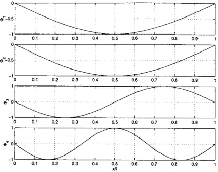
frequen-Comparing the results with those obtained in (1), we find that the absorber causes the first natural frequency to split into two but has little influence on higher order natural frequencies. Figure 2-6 shows the first four mode shapes and indicates that the first two mode shapes corresponding to the first two natural frequencies are sim-ilar. The mode shapes as drawn do not show the position of the absorber which is in phase with the beam for the lowest frequency and out of phase for the second frequency.

0 10 20 30 40 50

(I)

60 7o 8O 90 100

Figure 2-5: The determinant of the transfer matrix versus frequency

- ... .--. ......................-. .----. ..--- ---. -- ... -... -... --. - -- ---... ... ... ... .. ... ... . ... '.... 9 8 7 a 6 5 4 3 2 IU

(36)

0 0.1 0.2 0.3 0.4 0.5 0.6 0.7 0.8 0.9 1 0-0 0.1 0.2 0.3 0.4 0.5 0.6 0.7 0.8 0.9 1 0 01 02 03 04 05 06 07 0.8 0.9 1 S 0 ---. - -. --...---.. .--.-.--.- -.-0 0.1 0.2 0.3 0.4 0.5 0.6 0.7 0.8 0.9 1 x/I

Figure 2-6: The first four modes of the composite system

(3) Steady-state response of a free-free pipe structure

Case (a): A uniform free-free pipe The parameters of the pipe are as follows: Length: I = 6.10 m;

Outer diameter: d0 = 0.0230 m;

Inside diameter: di = 0.0206 m;

Bending rigidity: EI = 1.0284 x 103 N.m2_{; and}

Amplitude of the exciting force at the left end: po = 1000 N.

Figure 2-7 shows the transfer mobility (aRL) _{versus frequency. The mobility}(&RL)

is the harmonic velocity at R due to a unit exciting force at L. We calculate the velocity amplitude of the right end due to the unit harmonic exciting force at the left end. The peaks correspond to the natural frequencies. The first elastic natural frequency found from this figure is 3.84 while the analytical solution is 3.83. Other natural frequencies are all close to those analytical values.

(37)

20 10 0 i-10 -20 -30 -. -- - --- -- -6 8 1 1 0 4 6 20 40 60 80 100 120 140 160 -40 .0oo

Figure 2-7: The transfer mobility of the free-free pipe

Case (b): A uniform free-free pipe with mass attachment at midpoint

On the basis of the free-free pipe in (a), we attach a concentrated mass (m=1.40 kg)

at the midpoint, shown in Figure 2-8. Figure 2-9 shows the transfer mobility (C'RL)

versus frequency. The result in (a) is also included for comparison.

-Or1

m

-Figure 2-8: The simply-supported constantly tensioned uniform beam attached by a mass-spring absorber at the midpoint

For a free-free beam, the midpoint is a node of even elastic modes. Hence, for the even elastic modes, the mass attachment has no influence. Figure 2-9 indicates that

(38)

20 10 0 -10 -20 -30 -401 0 20 40 60 80 100 120 140 160 (0)

Figure 2-9: The transfer mobility of the free-free pipe with mass attachment the natural frequencies of the even elastic modes are identical and that the mobility peaks coincide at the frequencies. For odd elastic modes, the midpoint is not a node. The mass attachment influences the old elastic modes, and it increases inertia of the system. Thus Figure 2-9 shows that the natural frequencies of the odd elastic modes are lower than in the case without the mass attachment.

2.4 _{Wave reflection and transmission in a beam}

structure due to discontinuities

2.4.1 The derivation of wave reflection and transmission

ma-trices

The equation of motion of a uniform beam under constant tension is:

- - -- - -. --. -. - . -.. -.

- -.

-. --... -.

with mass attachment no mass attachemnt

A .. .. .. . . . .... ... .. ... ..

It ...

It .. .

(39)

-where y(x, t) is the displacement of the beam, El is the flexural rigidity, pA is mass

per unit length of the beam, and T is the tension. The shear force

Q

and bending

moment M are:

Q

= EId3_y/0X3 _- _T_ay/Ox, _M₌_EIa2_y/0x2_. _(2.19)

Assuming y(x, t) = ei(kx-iwt), and substituting it into Eq. (2.18) results in the

following dispersion relation:

EI k4 _{+T k}2 _{- pAw2 =,} _(2.20)

where the propagating wavenumber k1 and evanescent wavenumber k2 are:

1 T 1 T p w2

k 2 EI E 4 E

1 T T PAW2

k2= i1 -( I)2 + l)4 + (2.21)

The solution to Eq. (2.18) can be written as the sum of four flexural wave components:

y(x, t) = (a+e-iklx + a-eiklx + a+ e-k2x + aek2x )eiwt, (2.22)

where the amplitude a may be complex. The a+ and a- represent respectively going and negative-going propagating waves and the a+ and a- are positive-and negative-going attenuating waves which decay exponentially.

As in [26], we group the wave amplitudes into 2 x 1 vectors of positive-going waves a+ and negative-going waves a-:

a+ - a

a+N

Dynamic stiffness and transfer matrix analysis of marine riser vibration

Dynamic Stiffness and Transfer Matrix Analysis of Marine

Riser Vibration

by

Yongming Cheng

Submitted to the Department of Ocean Engineering

in partial fulfillment of the requirements for the degree of

Doctor of Philosophy

at the

MASSACHUSETTS INSTITUTE OF TECHNOLOGY

January 2001

@

Yongming Cheng, MMI. All rights reserved.

The author hereby grants to MIT permission to reproduce and

distribute publicly paper and electronic copies of this thesis document

in whole or in part.

Signature Redacted

Author...

Department of Ocean Engineering

January 24, 2001

Signature Redacted

C ertified by

...

..

...

J. Kim Vandiver

Professor of Ocean Engineering

Thesis Supervisor

Signature Redacted

Nicholas Patrikalakis

Kawasaki Professor of Engineering

Chairman,

partment Committee on Graduate Students

APR 18 2001]

AFC

Dynamic Stiffness and Transfer Matrix Analysis of Marine

Riser Vibration

by

Yongming Cheng

Abstract

Acknowledgments

Contents

List of Figures

f

List of Tables

fr,,

Chapter 1

Introduction

1.1

Problem Statement

1.2

Technical Summary of Numerical Methods

1.3

Overview of this thesis

Chapter 2

Transfer Matrix Method

2.1

Introduction

2.2

An outline of the transfer matrix method

2.2.1

state vector and transfer matrix

Q

Q

F

2.2.2

Eliminating intermediate state vectors and finding

fre-quency determinant

Q

Q

2.2.3

Response analysis

Q

2.3

Vibration analysis of a beam structure with

discontinuities

m

2.4

Wave reflection and transmission in a beam

structure due to discontinuities

_Chairman,

_{partment Committee on Graduate Students}

_{Wave reflection and transmission in a beam}