Dynamic trading and manipulation in financial markets

Dynamic Trading and Manipulation in Financial

Markets

by

Kan Huang

B.A. Mathematics, University of Cambridge (2006)

Submitted to the Sloan School of Management

in partial fulfillment of the requirements for the degree of

Doctor of Philosophy

at the

MASSACHUSETTS INSTITUTE OF TECHNOLOGY

June 2011

@

2011 Kan Huang. All rights reserved.

The author hereby grants to MIT permission to reproduce and

to distribute publicly and electronic copies of this thesis document in

whole or in part.

IMAS SACHUVEJ rTL OF TJC Y

L BRRE

ARCHIVES

Author ..

Sloan School of Management

26 Apr 2011

Certified by ...

Accepted by...

Will

v

u

IJiang Wang

Mizuho Financial

oup Professor

esis Supervisor

R

rto M. Fernandez

iam F. Pounds Prof

Lsor

in Management

Dynamic Trading and Manipulation in Financial Markets

by

Kan Huang

Submitted to the Sloan School of Management on 26 Apr 2011, in partial fulfillment of the

requirements for the degree of Doctor of Philosophy

Abstract

Chapter 1 studies how asset managers, due to reputation concerns, manipulate perfor-mance through taking latent risk dynamically. It is found that both skilled and unskilled managers load on excessive level of latent risk to boost performance even if investors are fully rational. The equilibrium risk taking by managers has interesting implications on investors' evaluation of manager's skill under normal market conditions and upon crash. Excessive risk taking reduces welfare of investor as well as unskilled managers, which calls for the presence of diligent third-party monitoring. Time required by investors to discover a manager's ability is also significantly lengthened. Our model yields several unique pre-dictions about crash losses, which are supported by empirical analysis using hedge fund data. Besides, it provides complementary explanations for declining returns of large funds and the high demand for structured mortgage securities before the subprime mortgage crisis.

Chapter 2 investigates price manipulation in general equilibrium with the only market im-perfection being the presence of a non-competitive large trader. We propose the notion of "pure manipulation", in which the large trader manipulates security prices to improve-her welfare but supported by no genuine trading motive. The existence of pure manipulation is equivalent to the failure of the Weak Axiom of Revealed Preference of aggregate security demand at the competitive equilibrium. We state conditions that prohibit pure manip-ulation. We also demonstrate that heterogeneity in preferences and endowments, large trading needs and remaining insurance demand in the competitive equilibrium could lead to a jointly upward-sloping portfolio demand, which gives rise to pure manipulation that requires arbitrarily small capital commitment. In addition, we establish a link between static and multi-period manipulation and show that dynamic trading reduces manipu-lation power. Different security structures that complete the markets lead to different equilibrium allocations in the presence of a non-competitive trader.

Chapter 3 analyzes how a risk-averse large institutional investor with price impact trades dynamically in the presence of momentum traders. The larger investor engages in several interesting manipulative behaviors. She may conduct "round-trip" trades to profit from momentum sentiment. She may buy (sell) before planned large sale(purchase) to ma-nipulate intertemporal demand. In addition, she takes profit less aggressively to let the momentum sentiment last longer. Besides, with endogenously generated price impact, we find that higher price volatility does not lead to faster execution.

Thesis Supervisor: Jiang Wang

Acknowledgmets

I am deeply grateful to my thesis advisor Jiang Wang for his guidance, encouragement

and support. I am also very grateful to my committee members Leonid Kogan and Hui Chen for many insightful advices and helpful suggestions. I would like to thank Randy Cohen, Scott Joslin, Andrew Lo, Konstantin Milbradt, Jun Pan as well as other faculty members of the Sloan finance department for invaluable discussions. I would also like to express my gratitude towards my fellow PhD students Jack Bao, Winston Dou, Xing Hu, Brandon Lee, Yichuan Liu, Indrajit Mitra, William Mullins, Zhihua Qiao, Weiyang Qiu, Hong Ru, Yang Sun, Ngoc-Khanh Tran and Amy Zhou for many useful conversations.

Contents

1 Reputation Concerns and Performance Manipulation With Latent Risk 1.1 Introduction

1.2 Related Literature . . . . 1.3 Model Setup . . . .

1.4 Solution of the Equilibrium . . . . 1.4.1 Investors' Learning . . . . 1.4.2 Manager's Maximization . . . . 1.4.3 Equilibrium . . . .

1.5 Analysis of the Equilibrium . . . . 1.5.1 Naive Investors . . . .

1.5.2 Semi-Rational Investors . . . . 1.5.3 Fully Rational Investors . . . .

1.6 Implications of the Equilibrium . . . . 1.6.1 Inefficiencies . . . . 1.6.2 Other Implications . . . . 1.7 Fund Termination . . . . 1.8 Empirical Analysis . . . . 1.8.1 D ata . . . . 1.8.2 Idiosyncratic Component . . . .

1.8.3 Testing The Predictions . . . . 1.8.4 Robustness Checks and Discussion

1.9 Conclusion . . . .

2 Price Manipulation In General Equilibrium

2.1 Introduction . . . . 2.1.1 Related Literature . . . . 2.2 Static Economy . . . . 2.2.1 Model Setup . . . . 2.2.2 General Manipulation . . . . 2.2.3 Pure Manipulation . . . .

2.3 Extension To Multi-Period Economy . . . .

2.3.1 Model Setup . . . .

2.3.2 Security Structures . . . .

2.3.3 Pure Manipulation In Commitment Equilibrium 2.4 Conclusion . . . . . . . . 9 63 63 65 67 67 71 74 92 92 94 98 100 . . .

3 Dynamic Trading With Price Impact In The Presence of Momentum Traders 116 3.1 Introduction ... ... 116 3.2 Model Setup ... ... 119 3.2.1 Investment Opportunities ... 119 3.2.2 Investors . . . .. 120 3.2.3 Timeline of Trading . . . . 121

3.3 Equilibrium Definition and Solution . . . . 122

3.3.1 S-Investors' Problem . . . . 122

3.3.2 L-Investor's Problem . . . 123

3.3.3 Solution of the Equilibrium . . . 123

3.4 Equilibrium Results . . . 126

3.4.1 All Investors Are R-Investors . . . 127

3.4.2 I-Investors Trading Against R-Investors . . . 127

3.4.3 R-Investors Trading Against L-Investor . . . 128

3.4.4 I-Investors Trading Against L-Investor . . . 131

List of Figures

1-1 1-2 1-3 1-4 1-5 1-6 1-7 1-8 1-9 1-10

Optimal Latent Risk Exposure (Against Naive Investors) . . . . . Effect of Idiosyncratic Volatility (Against Naive Investors) . . . .

Updating Sensitivity (Against Semi-Rational Investors) . . . . Optimal Latent Risk Exposure (Against Semi-Rational Investors) Optimal Latent Risk Exposure (Against Fully Rational Investors) Component in L-type Value Function Due to Reputation . . . . .

Pdf of Post-Crash Reputation when

pt

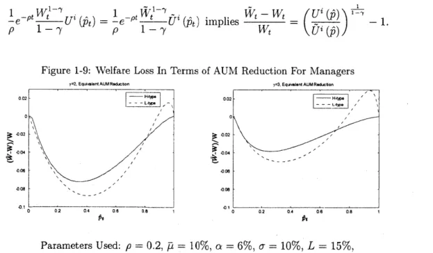
= 0.5 . . . .

Effect of Idiosyncratic Volatility (Against Fully Rational Investors) Welfare Loss In Terms of AUM Reduction For Managers . . . . . Welfare Loss In Terms of AUM Reduction For Passive Investors .

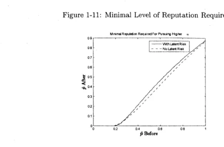
1-11 Minimal Level of Reputation Required . . . .

1-12 Minimal Level of Reputation Required . . . . 2-1 Complete Insurance . . . . 2-2 Numerical Illustration With General Utility Functions . .

2-3 CRRA Utilities . . . .

E[Qt) and Vart[Qt+i] for I-Investors v.s. R-Investors . . Autocorrelation for I-Investors v.s. R-Investors . . . . L-Investor's Holding Trajectories After A Position Shock R-Investor's Holding Trajectories After A Position Shock

Corr(Tradet, APt) . . . .

Trajectories After A Dividend Shock, With L-Investor . Trajectories After A Dividend Shock, With R-Investors Coefficient on Lt in L-Investor's Strategy . . . . Expected Excess Return and Conditional Variance . . . .

Coeffients On Multiple Past Excess Returns . . . .

. . . 128 . . . . . . 129 . . . . 133 . . . 134 . . . 134 . . . 135 . . . 136 . . . 136 . . . 137 . . . 138 3-1 3-2 3-3 3-4 3-5 3-6 3-7 3-8 3-9 3-10

List of Tables

Expected Discovery Time . . . . Dow Jones Credit Suisse Indices Return . . Hedge Fund Benchmark Factors . . . . Seven Factor(plus Lagged Mkt) Regression Large Residual Tests( > 3 Residual Vol) .

Different Cutoffs For Large Residuals . . . . "Live" and "Graveyard" Subsamples . . . .

. . . 3 7 . . . 4 2 . . . 4 4 . . . 4 7

. ... .. .. . .. .. . .. .

5 0

. ... .. .. . .. .. . .. .

5 1

. . . . 5 2 2.1 Efficiency Implications . . . 73 2.2 Dynamic Equilibrium Under Various Complete Markets Security Structures 98

Chapter 1

Reputation Concerns and

Performance Manipulation With

Latent Risk

1.1

Introduction

Since the demise of LTCM in 1998, strategies that generate steady returns under normal market conditions but incur large losses upon occasional crashes have caught researchers and practitioners' attention. The "Quant Meltdown"' in 2007 provides another vivid example: several popular statisitical arbitrage strategies, which were supposed to yield "arbitrage-like" returns with relatively small risk most of the time, suffered tremendous losses when the whole sector was caught in a wave of unwinding. In 2008, people witnessed huge losses from senior tranches of mortgage securities and credit derivaties, which had delivered stable returns before the recession and the collapse of house price. These events beg for the same question: why causes the proliferation of securities or strategies containing significant amount of risk that is latent in nature? While it could be potentially due to neglected disaster risk as argued in Gennaioli, Shleifer and Vishny (2011), the collapse of JWM Partners, a second fund set up by the former LTCM founders, suggests the possilibity of alternative explanations. This paper attempts to address the question from the perspective of reputation concerns and associated fund flow.

As Mark Hurley from Goldman Sachs once wittily remarked, "the real business of money management is not managing money, it is getting money to manage." Indeed, an important factor to the success of asset management is to grow asset under management (AUM) and collect fee on a larger base. Several papers2 have empirically documented that money flows in or out of funds after good or bad performance. As Berk and Green (2004) demonstrated, such flows can be explained by investors' update of managers' ability after observing fund

'Several famous quantitative players such as Morgan Stanley's Process-Driven Trading group and Goldman Sach's Global Equities Opportunities Fund posted large losses.

2

Chevalier and Ellison (1997), Sirri and Tufano (1998) have studied mutual fund data and found that fund flow has been strongly correlated with past returns.

performance, which we shall refer to as "reputation". Reputation concern creates an implicit incentive for managers, which induce them to behave inefficiently. This paper focuses on the effect of reputation concerns on risk taking in the presence of securities or strategies that deliver steady positive returns under normal market conditions but incur potentially large losses upon market or liquidity crashes. We shall refer to this distinct type of risk-return profile as "latent risk", which generalizes over strategies that are often referred to as "insurance selling" or "nickel-picking".

There are several sources that give rise to latent risk. Firstly, it could be simply due to the pay-off profile. For example, credit default swaps and out-of-money put, by design, contains significant amount of latent risk. So do structured products such as senior tranches of mortgage securities, which are termed as "economic catastrophy bonds" in Coval, Jurek and Stafford (2008). Secondly, latent risk could arise endogenously for well-known strategies. An inherently good strategy that generates steady return with little risk naturally attracts many fund managers. When a large player of such a strategy is hit, she is forced to liquidate to meet the margin constraint. This might engender the "margin spiral"3, which underlies the "Quant Meltdown" and the occasional bad performances of carry trade. Finally, latent risk could be caused by illiquid assets such as bespoke synthetic CDOs that are marked up steadily but register a sharp fall in value when there is a liquidity crash.

Latent risk is of particular interest in the context of performance manipulation because its unique risk-return profile allows managers to boost performance without getting detected until a rare crash. In this paper, we study the optimal exposure of latent risk taken by risk-averse asset managers in a Bayesian rational equilibrium with information asymmetry. An asset manager running a certain type of fund follows a pre-specified strategy stated in the fund prospectus, the risk-return profile of which is known to the investors. A manager could be skilled or unskilled, which is only known to herself but not to investors. Skilled manager can generate an alpha in excess to the pre-specified strategies' expected return. In addition to following the pre-specified strategy, manager can load secretly on latent risk, which boost instantaneous return with little volatility at the expense of a large loss upon crash. Investors cannot observe the level of latent risk-taking by manager but they can form conjecture about it. What they are able to observe is the overall fund returns. Thus, they have to constantly update the reputation4 _{of a manager during normal times}

and upon crash in a Bayesian manner. With fund flow increasing in reputation, it becomes an important concern for managers.

While it is expected that managers without skill choose to manipulate performance by taking excessive (relative to the pure risk-return optimal) latent risk exposure, managers with skill also engage in such behavior, which is puzzling given that they possess genuine alpha-generating ability. The reason is simple: since the unskilled manager will never attempt to generate higher expected return than a skilled one, the equilibrium updating rule by investors always rewards higher realized return with higher reputation. Uable to

3

See Brunnermeirer and Pederson (2008).

convince investors about their skill due to information asymmetry, the skilled managers optimally choose excessive latent risk exposure to expedite the type discovery. In general, managers with skill take less latent risk exposure than managers without skill under concave utility. However, interestingly, when a skilled manager's reputation is sufficiently low or on the brink of fund termination, the skilled manager may aggressively take even more latent risk to avoid being nailed down to an unskilled one or forced to shut down after a few unfavorable return shocks. Thus, a somewhat unexpected implication is that, when a manager's reputation is already low, a rational investor should not always lower the manager's reputation upon observing a large crash loss.

Rational updating by investors, especially upon crash loss, is very effective at reducing the gap between latent risk exposures taken by skilled and unskilled managers. This is because learning the expected return under Gaussian noise is notoriously slow whereas the information revealed from a crash loss could be substantial. If the unskilled managers take on significantly more exposure than the skilled ones, the gain from boosting the expected return during normal times is outweighed by the loss of reputation revealed by a large loss upon crash. In addition, unskilled managers do not wish to suffer a reputation setback concurrent with large financial loss. These lead to a "noisy pooling" equilibrium, in which the unskilled managers' optimal latent risk exposure is riot significantly different from that of the skilled ones. Consequently, the equilibrium evolution of reputation is relatively gradual despite that crash happens rather abruptly. This implies that rational learning alone may not be able to fully explain the drastic withdrawal commonly observed after a fund suffers a substantial loss.

Deviation of latent risk exposure from pure investment optimal creates inefficiency in risk taking. In equilibrium, rational investors can discount the latent risk return from realized performance qutie accurately given the "pooling" nature of the equilibrium. As a result, managers cannot gain much reputation although they take excessive latent risk. This calls for the presence of a third-party, who can monitor the risk position of a fund closely and certify to investors that the level of latent risk taking is appropriate. This also justifies the use of investment mandate, which, if effectively enforced, makes performance manipulation through latent risk much more costly. Such self-commitment implementations are in the interest of managers and worth up to 8% of AUM for a manager with mediocre level of reputation. More importantly, the damage to investors' welfare is also substantial. Depending on the level of information asymmetry, the equivalent welfare loss due to excessive latent risk exposure could be up to 7% of money invested. In addition, it is found that latent risk can significantly lengthen the type discovery time by around 30% since higher latent risk exposure taken by unskilled managers in equilibrium reduces the differential expected return and, therefore, the information content of fund performance. This engenders inefficiency in fund flow.

Our model generates a few unique empirical predictions on crash loss, which is related to the level of latent risk exposure. The optimal level depends on the sensitivity of investors' updating rule. Higher updating sensitivity increases the incentive to boost reputation through latent risk exposure. There are a few factors that determine the updating sensi-tivity. Higher idiosyncratic volatility adds noise to observed fund returns whereas larger

difference in alpha-generating ability between skilled and unskilled managers increases the information content of fund returns. Thus, the former has negative effect and the latter has positive effect on updating sensitivity. Furthermore, when investors are certain of a manager's type (i.e. when reputation is very high or low), they do not weigh much on new observations of fund return, which lowers the sensitivity. Using the TASS dataset for hedge fund returns, we test our predictions and show that the data is consistent with our model predictions.

Besides, previous empirical studies have documented that larger fund has declining return. It is most commonly attributed to trading cost and decreasing return to scale. Our model complements these explanations with a novel one: larger funds tend be those with high reputation and, as a result, take less latent risk, which reduces the expected return during normal times and overall5_{. Our model also provides an explanation for high demand of}

mortgage-backed securities, which contributed to the subprime mortgage crisis. Mortgage-backed securities exhibits typical latent risk features. And, with liquidity awash during the period of 2002-2006, new funds were set up and they demanded latent risk. Also, as the overall prior reputation decreased due to limited supply of skilled managers, this further pushed up the demand for latent risk as lower reputation would increase latent risk exposure in general.

This paper is organized as follows: Section 1.2 discusses the related literature. Section 1.3 presents the model setup. Section 1.4 discusses the solution of the equilibrium. Section 1.5 focuses on the analysis of latent risk exposures taken by managers in equilibrium. Section

1.6 considers the implications of the equilibrium. Section 1.7 considers a impact on latent

risk exposure if fund termination at low level of reputation is introduced. Section 1.8 tests several implications empirically. Section 1.9 concludes. Proofs and numerical procedures are contained in the Appendix.

1.2

Related Literature

With the rise of hedge fund industry, the presence of latent risk, which is easily

accessi-ble to hedge fund managers, has attracted people's attention. Malliaris and Yan (2010),

Makarov and Plantin (2010) as well as He and Xiong (2010) have approached this issue from different perspectives. Our paper is closely related to Malliaris and Yan (2010), which also studies the excessive deployment of latent risk strategy due to reputation con-cerns in a discrete-time framework. While they only allow for binary choice of latent risk exposure, we analyze the case where manager can choose the optimal level of exposure from a continuum. This allows us to study the comparative statics and generate testable predictions. Moreover, the equilibrium implication on investors' learning process is dif-ferent. In their model, investors update positively on a manager's reputation regardless of her true type most of the time until a crash, which is accompanied by a large negative update. In contrast, investors in our model update on the manager's type in the correct

5

direction gradually over time. Makarov and Plantin (2010) finds that the optimal method to game convex compensation contract is through taking latent risk and considers various contracts with commitment to address this issue. He and Xiongs (2010) discusses the design of optimal investment mandate to restrict the manager from taking unnecessary latent risk.

Our paper belongs to the growing literature studying the impact of manager's reputation concerns on investment decisions (e.g., Stein and Scharfstein (1990), Dow and Gorton

(1997), Dasgupta and Prat (2006, 2008), Vayanos and Woolley (2008)). These studies

focus on how reputation concern distorts the use of private information for trading. Our paper focuses on the effect of an outside investment opportunity, namely latent risk, on risk taking.

More broadly, our paper is also related to the large body of literature on managerial incentive that either takes the form of compensation contract (e.g. Jensen and Meckling

(1976), Carpenter (2000), Ross (2004), Panageas and Westerfield (2009)) or explicitly

specified fund flow function (e.g. Basak, Pavlova and Shapiro (2007, 2008), Basak and Makarov (2009), Chapman, Evans, Xu (2009)) in partial equilibrium. Several papers have also considered the asset-pricing implications in a general equilibrium framework (Arora, Ju and Ou-Yang (2006), Cuoco and Kaniel (2010), Guerrieri and Kondor (2010), Kaniel and Kondor (2010)). Optimal contract has been designed under specific scenarios (e.g. Ou-Yang (2003), Cadenillas, Cvitanic and Zapareto (2007), Dybvig, Farnsworth, Carpenter (2010)) to handle incentive problems.

Finally, performance manipulation against common measures such as Jensen's a or Sharpe ratio has been analyzed in Goetzmann, Ingersoll, Spiegel and Welch (2007) and Guasoni, Huberman and Wang (2010). Lo (2001) also considers a simple option-writing strategy that delivers high Sharpe ratio. Our paper adds to this branch of literature by studying the effect of latent risk, which has the unusual negatively-skewed risk-return profile, and endogenizing the performance measure through rational Bayesian updating.

1.3

Model Setup

In this section, we shall formulate our model in a continuous-time dynamic setup. We shall specify the details of the investment opportunities faced by a fund manager and investors' learning about manager's ability.

Pre-specified Strategy

A fund manager has expertise in a particular strategy that falls into some well-known

investment style. She states her expertise in the fund prospectus and follows the strategy of her specialty. We shall refer to this strategy as the "pre-specified strategy". Let Rt denote the the cumulative fund return per dollar (after fee). Equivalently, it is the value at time t of an $1 investment in the fund made at time 0. Under the pre-specified strategy,

we assume that Rt follows a geometric brownian motion with jump

d Re

R = pdt + odB + (e-L - 1) dAt (1.1)

fT is the expected return (after fee) of the pre-specified strategy. We assume that p is

known to investors since they are familiar with the investment style, which determines the expected return of the pre-specified strategy. o is the volatility of the fund return and

Bt is a standard Brownian motion. oBt captures the inherent Gaussian risk in the

pre-specified strategy. It could be a combination of both systematic risks and idiosyncratic risk. As investors can disentangle the systematic risk component perfectly in continuous-time by comparing the fund return process with the return processes of systematic risk factors, loadings on systematic risk factors play no role in investors' learning process. Thus, for simplicity, we shall assume that uBt is purely idiosyncratic, which depends on the specific implementation by the manager and cannot be observed directly by investors.

Nt is a standard Possion process with intensity A. If Nt jumps at t, it represents a

market/style-wide crash that affects the pre-specified strategy. It has been well-documented that the overall equity market carries significant crash risk. In addition, the "quant fund crisis" in 20076 demonstrates that certain styles of strategies could have substantial crash risk due to the downward margin spiral of market liquidity and funding liquidity. Upon on a crash, the fund's cumulative return Rt falls to a fraction e-L-6 of that before the crash:

R = e-LRt- where L > 0 is the mean size (logged) of the crash loss and e ~ N (0, oC)

is the idiosyncratic jump loss. A market/style-wide crash has different impact on indi-vidual funds. While funds belonging to a certain style suffer a loss of L on averge, the extent, to which an individual fund is affected by the market/style-wide crash, depends on what portfolio that particular fund holds at the time of crash. Thus, there is an idiosyn-cratic component e in the jump loss. Moreover, as market/style-wide crashes are rare and caused by different underlying problems from time to time, we can treat e's to be I.I.D over time. Since investors are familiar with the investment style that the pre-specified strategy blongs to, L is known to investors. However, due to its idiosyncratic nature, e is not observable to investors.

Manager's Skill

We assume that a manager could be skilled or unskilled in the strategy style she specializes in. A skilled manager (referred to the "H-type") adds an alpha to fund return on top of what is generated by the pre-specified strategy whereas an unskilled manager (referred to as the "L-type") adds nothing. Here, we do not model the source of alpha, which could come from superior information or ability to identify potential arbitrage opportunities. Therefore, under the management of a H-type manager, the cumulative return process has higher drift

dRt

Re=(a+fp) dt +od Bt+ (eL* - 1) dNe

6

whereas, under L-type, the return is the same as that of the pre-specified strategy. a > 0 is the incremental return contributed by a skilled manager.

In general, we shall write the cumulative return process as

R = pidt + adBt +

(e-

dNt, i = H, L (1.2)

where

pi = p + a" and aH a,aL 0

We assume that manager knows her type whereas investors cannot observe it. This is motivated by the fact that manager has substantial knowledge of how her strategy is conducted and whether it possesses any alpha through simulation and backtesting. Also, she might have extensive previous trading experience before. Of course, it is possible that sometimes a manager is overconfident and believes that she has alpha-generating ability, which, in reality, she does not possess. Nevertheless, it is still quite reasonable to assume that manager has much better knowledge about her skill level than investors. Thus, there is information asymmetry regarding the skill type of a manager.

Latent Risk

So far, the return of a fund depends on the risk-return characteristic of the pre-specified strategy and the type of the manager, which are completely exogenous. This is similar to Berk and Green (2004), in which manager does not actively control the return process. We shall now introduce latent risk and the manager can control her fund's exposure to the latent risk. Furthermore, we shall assume that her choice of exposure to the latent risk is over a continuous space rather than being confined to a few discrete levels.

Specifically, a unit of latent risk provides extra return of irdt over the time interval dt during normal market conditions but incurs a loss of A percent when crash occurs (i.e. when dNte = 1). We assume that 7r < A to emphasize on the skewed risk-return profile.

Here, there are two implicit assumptions made. Firstly, we assume that crash due to latent risk is concurrent with the market/style-wide crash (both are driven by Nt), which is usually true. For instance, if an equity-oriented fund loads on latent risk by selling out-of-money index put options, it is hit by latent risk loss exactly at the same time when the overall equity market crashes. Alternatively, if the latent risk is achieved through holding illiquid assets, then the crash loss caused by latent risk is again simultaneous with the liquidity crash. The same holds true for carry trade, which is known for incurring large loss when the whole investment style suffers from occasional massive unwinding7. Merger arbitrage is also found to suffer bad performance when the overall market condition turns sour8. The second implicit assumption is that latent risk generates positive return and negative jump losses with no volatility. In reality, some assets with latent risk might be marked to market frequently and, as a result, produce small Gaussian shocks under normal market conditions. But the Gaussian volatility generated by latent risk is usually

7

See Brunneimeier, Nagel and Pedersen (2009).

negligible compared to the volatility of the pre-specified strategy. Besides, if latent risk is taken through holding illiquid asset, which is not subject to the marked-to-market procedure, we shall not observe much volatility either. We ignore the Gaussian volatility associated with latent risk to focus on its distinctive feature that is different from the usual Gaussian type of risks.

It is worth noting that we should not consider latent risk taking in the narrow context of hedge fund managers only, who admittedly enjoy greater freedom in their choices of risk taking. A general pension or mutual fund manager could also access latent risk through marginal portfolio adjustment. For instance, an international bond fund manager can load on latent risk by reducing the portfolio weight of Japanese government bond and increasing the portfolio weight of Australian government bond. The marginal effect achieved is exactly a carry trade strategy. Similarly, many pension fund managers chose to hold senior tranches of mortgage securities rather than safer treasury bonds, which yielded a steady spread of 1-2% annually during years of economic boom and suffered almost no default loss. However, during the credit crisis, substantial loss was incurred due to collective default by borrowers as documented in Adelino (2009). In short, being able to load on latent risk should be regarded as a general phenomena among fund managers rather than the special previlege of hedge fund managers alone.

Latent risk is of particular interest to managers because usual risk sources (say aggregate equity market risk) generate greater return at the expense of greater volatility. With frequent observations of fund returns by investors nowadays (most commonly daily or weekly), variations in level of volatitlity can be detected by investors. Thus, if manager loads on the usual sources of risk, higher return will be discounted by investors, who notice the increase in volatility and understand that extra risk have been taken on. Therefore, they will not perceive the manager with higher reputation. Latent risk delivers return with relatively little volatility. Thus, investors cannot detect it unless a rare crash occurs. As argued in Lo (2007), a simple strategy of selling out-of-money index put options can deliver a significant positive alpha in an unsophisticated linear regression framework. Manager of type i can choose her exposure of latent risk

#

at time t where i = H, L. By

doing so, the instantaneous return during normal time will be incremented by irq'dt and the cumulative return process will be

dRe

R ( p=i +r#) dt + odB,

However, upon a crash, she will lose A#' more on top of the crash loss incurred by the pre-specified strategy:

Rt= I - Ae)

Putting together, the overall cumulative return follows

dRt _{- (pi + 7r#1) dt + odBt +}

_[(I

_{- Ad) e-"} L,

- 1] dN (1.3)

Investors cannot observe the precise level of latent risk exposure

#1

although they may form conjectures about it. While SEC requires quarterly disclosure of portfolio holdings with some lag in 13-F filings for funds with more than 100 million under management, investors can infer limited information from it. First of all, managers trade at much higher frequency than quarterly basis. Thus, the 13-F filings provides at most a snapshot of portfolio holdings, which changes on daily, weekly or monthly basis. This might be subject to the "window-dressing" efforts undertaken by fund managers as well. Secondly, short positions and many derivatives contracts are not required to be reported. Thus, investors cannot gather the full information about portfolio position. Last but not least, the source of latent risk can be obscured by the vast number of investment positions and complex financial contracts in the portfolio, which makes the inference problem even harder.

Learning By Investors

In summary, we have assumed that investors can only observe the cumulative return Rt

but cannot observe:

1. the type of manager

2. Bt and

E,

which are idiosyncratic to a fund

3. the choice of latent risk exposure

#'

by manager

Thus, they try the learn the type of manager after observing the cumulative return from time 0 to t, R[o,t], and update the probability of the manager being a skilled H-type

pt

= Pr

(i

= HIR[o,t]) (1.4)

Et

[1{iH}1

where Ef [-] denotes the conditional expectation based on investors' information. Since there are only two types of managers,

Pt

fully captures the reputation of a manager.Thus, we shall refer to

Pt,

the posterior probability of a manager being skilled, and "reputation"

interchangeably.

Fund Flow and Reputation Concern

We assume that the fund flow rate is an exogenous increasing function

f

(Pt) to capture

the simple fact that fund flows into hands of managers with greater reputation. The purpose of introducing fund flow into our model is to provide a simple but realistic chan-nel for reputation to reward managers through greater asset under management (AUM). The fund flow is gradual in our model. This can be justified by costly search among some investors as argued in Sirri and Tufano (1998). Also, not all investors are actively monitoring the performance of the fund constantly. Moreover, even if investors are com-pletely sure that the manager is of L-type, they may still invest with the manager for diversification purposes. Though a H-type manager generates higher expected return,

there is still room for the presence of L-type manager following the same pre-specified strategy to reduce idiosyncratic risk. Finally, investors are wary of operational risk as pointed out in Brown, Goetzmann, Liang and Schwartz (2008). They are cautious with high concentration and will not delegate all of their assets to a few H-type managers only. This is illustrated by the fact that, when BlackRock acquires Barcap Global Investors, investors fled to avoid concentration9_{. For simplicity, let}

_f

_{(.) be linear and increasing in}

reputation

Pt.

We further assume that

f

(0.5) = 0 so that higher

Pt

(> 0.5) induces fund

inflow whereas lower 1t (< 0.5) induces fund outflow.

Let Wt denote the asset under management (AUM) of the fund. With fund flow taken into account, the AUM evolves as follows

dW _ dRt

--- --- + f (Pt) dt

Wt Rt

- (pti + 7r# +

f

(zt)) dt + -dBt + [(1 - A#|) e-L - 1 dANe (1.5)

Part of the growth in AUM comes from investment return. The rest comes from attracting fund flow with a higher level of

Pt.

Since a manager wishes to have higher AUM, fund

flow, which depends on

Pt,

introduces reputation concerns for the manager. Manager's Objective

We assume that managers receive a management fee as a fraction

#

of AUM Wt. Managers try to maximize constant relative risk aversion (CRRA) utility over fee received.

max Et

00

e~PS

"

ds

Here we assume that managers consume the fee she receives and abstract away the po-tential consumption-saving decision. Furthermore, as our focus is the effect of reputation concern on level of latent risk exposure, we assume that the fee is a simple fraction of the

AUM. In other words, we do not consider the effect of incentive contracts such as

sym-metric fulcrum fee seen among mutual funds or those involves high-water mark, which is popular among hedge funds. Also, we assume -y > 1 to avoid unrealistic excessive risk taking behavior. For CRRA utility,

#

does not matter. Manager effectively solves

*0 W1~Yl

max

Et

~PS " ds

(1.6)

011 - S

Definition of Equilibrium

An equilibrium is defined as

#t",

,

4

}

where $' is an adapted process denoting

the latent risk exposure taken by manager of type-i and b denotes the conjectured latent risk exposure of type-i by investors (who does not observe

#|)

such that

9

1. Manager of type-i's latent risk exposure

#

solves max~i E ePt W

tU

dt

2. Investors correctly conjecture manager's latent risk exposure

t=

#t

Vt, i = H, L

and form their belief about manager's type through Bayesian updating:

it = Pr (i = H

I

R[o,t])

1.4

Solution of the Equilibrium

With infinite horizon and CRRA utility, we look for a stationary equilibrium that is Markov with the state variable being

Pt.

Hence, the choice of latent risk exposure O," and

#f

should only depend on the reputation at time t,

pt.

In other words, they are time-invariant. As a result, we may drop the subscript t and denote the choice of latent risk exposure as

#H

(.) and

#L

(.). We shall verify later that this is indeed an equilibrium.

The equilibrium needs to be solved in 3 steps. First, we need to find out how investors update

Pt

given their conjectures about manager's choice of latent risk exposure. Second, we need to find out what is manager's optimal latent risk exposure

#'

taking as given the investors' updating rule. Finally, we need to find out the fixed-point equilibrium, in which manager of a given skill type chooses the optimal latent risk exposure and investors correctly conjecture managers' strategies.

1.4.1

Investors' Learning

Investors' learning takes two forms: updating under normal market conditions (dNt = 0)

and updating upon a crash(dNt = 1). When they update, they have to form a conjecture

about manager's strategy i for i = H, L. Let the difference between the the investors'

H - L

conjecture about latent risk exposures of the two types of manager be ZA =

#

-H . The

following proposition states the Bayesian updating rule based on investors' conjecture.

Proposition 1 Conditioning on no jump in time interval [t, t + dtl, the reputation of a manager evolves as:

dpi=t

# ()

(

t

_ E

)

(1.7)

where

(1 )El

___i = H] - El $ i_= L]

Proof. See Liptser and Shiryayev (1977). U

d-E[

[E ]

_{measures the unexpected return shock for investors, which could be due}

to the idiosyncratic Brownian shocks or the difference between the actual drift rate of the cumulative return process and that expected by investors. The former carries no information about the manager's skill type. However, investors cannot disentangle the two sources of shock because of information asymmetry.

measures the sensitivity of updating. Note that

#

is small when

P

is close to 0 or 1 and big when

Pt

is around 0.5. When

pt

approaches 0 or 1, it indicates that investors are very certain of manager's type and they no longer update much on the new fund returns. At

p

= 0 or ^ = _{1, they are completely certain and there is no updating at all. They}

are two absorbing states for the reputation process. When

P

is around 0.5, investors are least certain about the manager's skill type. As a result, the sensitivity of updating is high, which reflects the fact that additional piece of evidence is useful for determining the type of manager. Moreover, the sensitivity 0 is high for low U, which is intuitive. The less noise there is, the more information the shock carries. Finally,

#

depends on E [dRti = H] - E [dRt i = L , which is the difference in expected returns of the two

types of manager. This is a measure of how much information content the unexpected shock possesses. In equilibrium (investors correctly conjecture),

Pt

follows a martingale based on investors' information filtration. However, as the following proposition suggests,

Pt

is not a martinagle from a manager's point of view since she knows her type and the exact drift of d.

Proposition 2 For manager of type i, her reputation follows

dpit

=

# (lt)

(ai

+

irO

+ o-dBt

-

[fit (0 + 1r$H) H (1L

(rr

))

(1.9)

and

pt 1 -pi)a + 7rE (t)

# t()-lt (= (it)(1.10)

When there is a crash, there is a large amount of information revealed, which requires the second type of updating. Consequently, this causes

Pt

to jump. Suppose the after-jump cumulative return is a fraction X of the before-jump cumulative return: Rt = xRt-. From

investors' perspective,

x

= 1 - Ao e-L. Without the idiosyncratic loss e, investors will be able to infer the manager's type from the crash loss by backing out the latent risk exposure 0 .However, with the idiosyncratic loss, the overall crash loss is stochastic. As a result, they can only perform Bayesian updating.

Proposition 3 Upon a crash, investors update according to the following rule:

pt

= P'

t-

IX)

(1.11) in (1- _(-)

_f

9_ 2 +)exp [i In - 2L,

This has an interesting feature. Rational updating by investors may not imply an increase in post-crash reputation

Pt

upon seeing a higher fraction of wealth preserved (i.e. smaller loss) after jump if H-type manager is conjectured to have higher latent risk exposure:

8P' H L

-- < 0 if ( -)> 0"(t)

This is reasonable because if H-type is expected to load more on latent risk at t, then her loss upon crash at t is expected to be higher. Thus, higher loss (i.e. lower

x)

indicates a higher probability of being skilled.

By law of iterated expectation, for investors,

Pt

is still a martingale with stochastic jump:

Et [P (Pt-, x)] =

Pt-.

Manager can decompose

x

into component from her latent

risk-taking (1 - A$|_) and component from pre-specified strategy e-L". Thus, from the

perspective of the manager, the updating rule by investors becomes

Pt=

P (pt-,$,e)

H

~(1.12)

1.4.2

Manager's Maximization

Manager of type i takes investors' conjectures Ot as given and solves

max Et e- ds

subject to

dW

(p

+r# +

f

(Pt)) dt + odB + [(1 - A#) eLe - 1] dNt (1.13)

dpt = # (z3) (ai +7 ir + a-dBt - t (a +rH + (1 --

)

1L] (1.14)

+(P (fit-,#0',e -Pt-) dNt

where first equation describes how AUM evolves according to the risk-return profile of the pre-specified strategy the manager follows, the choice of latent risk exposure

#

as

well as the fund flow

f (Pt). The second equation describes the evolution of the manager's

reputation under investors' conjecture '

(-).

Proposition 4 (1)Manager's optimal latent risk exposure

_#'

is a function of

Pt

and in-variant over time.

(2)The value function of type i manager is of the form V' (W,

p, t)

= -Pt r We U (i9)

(3)

#' (Pt) and U' (1Pt) satisfy the Hamilton-Jacobi-Bellman equation:

0 =min p+ -p - A + (1 - -y) p + 7roi + f (fit) - Iyo.2) Ui

+1 ((a - apt) + (1 - ) .2 + r $i pt H (Pt) + (1 ~-it) L (ft)

+ I Or0 0 3 U; + -) (I I\ r(1--)i )]Iu

2 + Ae~-)- Eo [e~ U (P (Pt, i, ))] (1.15)

with # minimizing

[(1 - -y) U' + #U ] 7r# + Ae -(l)L (1 - A#|) 1 ^ Et [e-('7)*U (P (Pt, #, e))] (1.16)

Given the form of value function and our restriction that

y

> 1, we can easily deduce that U' > 0 since V' should be increasing in AUM Wt, which implies

- = -e~' Wr-Ui _{> 0}

Also, we can conclude that U. < 0 since V' should be increasing in the reputation of the

manager

OVi

1

W

'-? =_ - e~p t Ui > 0

9t p 1 - P

The terms to be minimized by

#'

have very intuitive meaning. Loading on latent risk at level # could boost the fund return by 7r#|. (1 - y) U'7r#5 reflects the direct pecuniary

benefit from the steady return the latent risk factor provides. Also, with return

7r#dt

is reflected in the term #TrOiU,. Since (1 - -y) U' < 0 and Ui < 0, higher

#'

leads to lower

value of the first two terms of (1.16). Ae-(l)L (1 - Ao') 1' Et [e-(1Y) Ui (P (t,

#i

E))]

is a positive term, which counterbalances the linear negative effect of the first two terms and represents the cost of latent risk. A (1 - A$') ' measures the financial loss (after adjusted for risk-aversion) due to latent risk exposure when crash arrives(with intensity

A). This is combined with the loss due to pre-specified strategy e(1

Y)L (adjusted for risk-aversion) and expected investors' updating Et

[e*l)eUi (P (pt, #,

e))] upon a crash.

1.4.3

Equilibrium

If

Pt

= 0 or 1, when

Pt

will no longer change since investors are already completely certain of the types. So there is no reputation concern at all. Managers will simply choose the optimal latent risk exposure based on the pure risk-return trade-off. In other words, they will grow the AUM in an "organic" manner.

Proposition 5 If it = 0 or 1, L(+ 12 ct~ A (i)(1.17) U1 (0) U (1) p

p+ A + (y - 1) (pi +7r + f (0) -

jyo2)

- i (1 - A#)

p+A+(y- 1) (pA +r#+ f (1) - jyU2) - I (1 -A#)

(1.18) (1.19)

with a parametric restriction that

p+A+(y- 1) t+7r

+ f (0)

-

YO

-

(1-A#) > 0

Note that without reputation concern, the level of latent risk-taking is constant and the same for both types. It is straightforward to see that that the exposure increases in n, which is the premium of latent risk. Also, under the parametric assumption that y > 1, it is decreasing in the mean logged loss of the typical strategy L. This is understandable since manager is quite risk-averse(-y > 1). Given a loss will be incurred by the pre-specified strategy when a-crash arrives, it is undesirable to aggravate the situation by incurring further loss from latent risk exposure. Finally,

e

is decreasing in o,, the idiosyncratic jump loss due to risk aversion.

Proposition 6 In equilibrium,

i (P3

) = $

(p,).

Define A =

#OH

(fit) -

#L

($t). So the above equations simplifies to a fixed-point problem of differential-integral equations

0 = p+ p-A+(1 -7) pH + " + f - 2 UH U

2

+{ae (-)+ (1- ) U2 + 7r (1H - t f) + - 2o2U

+Ae-( -,y)L (igH17E e07""( "

)]for

i =H (1.20)

0 =p+ p-A+(1-7) P + L t - 7 L

2

+{afit + (1 - _Y) 02 -rpt A (pt)}I UP + 2 2U

+Ae~(~y)L (1 7AL) Et [e-(~7)UL (P (₁3t cLJe))] for i = L (1.21)

0= arg min r [(1 - y) Ui + OUj] # + Ae-(l-)L - Ao) '^ Et [e-(l-)Ui (P)] (1.22) with boundary conditions at 0 and 1 specified by (1.18) and (1.19).

The fixed-point involves three parties: potential H-type, potential L-type as well as the investors. We require both types of managers to maximize their utility while investors correctly conjecture. Due to the non-linearity and the involvement of integral (i.e. the ex-pectations that appear in the equations above), we have to resort to numerical techniques. The details are included in Appendix.

1.5

Analysis of the Equilibrium

In this section, we shall analyze the equilibrium solved in the previous section. As the

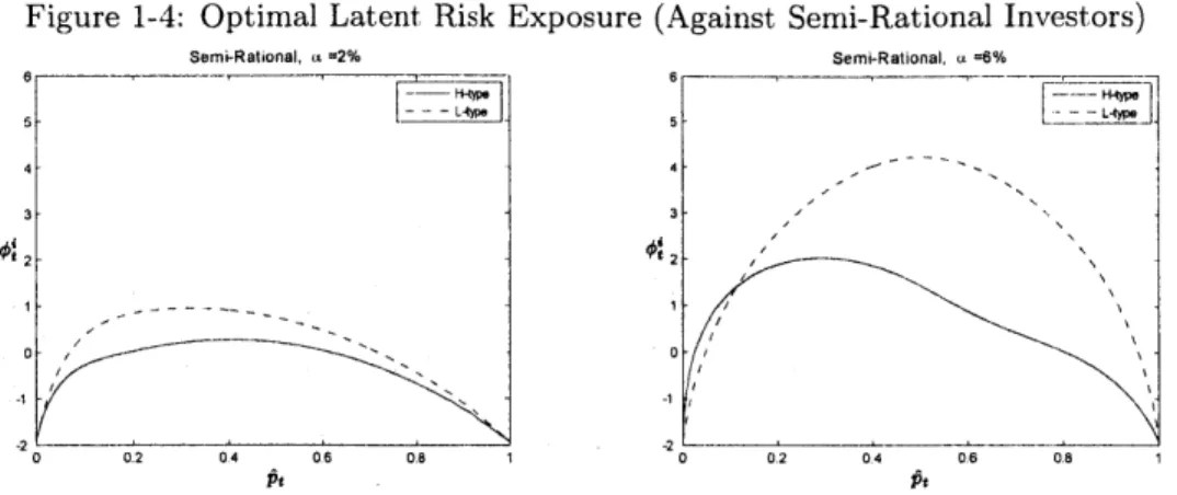
the equilibrium is a functional fixed-point problem involving three parties (potential H-type, potential L-type and investors) and two different forms of updating by investors, we shall analyze step by step to see the effect of each component. We start by analyzing an open loop case first - manager facing naive investors, who "naively" believe that managers will simply follow the pre-specified strategy and refrain from loading on excessive latent risk. This case will yield several basic intuitions, which still holds in fully rational equilibrium. Next, we shall consider the case, in which investors are semi-rational in the sense that they conjecture the latent risk exposure

#'

correctly to perform continuous-time updating but ignore the information content in jump loss. Finally, we consider the case in which fully rational investors conjectures

#'

correctly and perform updating both during normal market conditions and upon crash. This opens a potentially important channel for investors to learn about manager's skill type. We shall see that the equilibrium result is "noisy pooling", in which the difference in expected crash loss between H-type and L-type is small relative to the idiosynacratic noise.

1.5.1

Naive Investors

As long as investors do not perform jump updating, which applies for both the naive and semi-rational investors cases, the reputation levels before and after a crash is the same:

P

(ft,

di,

e)

=

Pt.

From (1.16), we find that the optimal latent risk exposure by manager of type i is

eq

2-y 7r Y +l

1 - e6( F( U

d A (1.23)

Since (1 - ) < 1 and < 0, we have 5--- > 0. Comparing this with (1.17), we see

that

4 (pt) ;>

with equality holds only when Pt = 0, 1. This suggests that managers always take on

excessive latent risk exposure than what is optimal without reputation concern. The

'3U'

magnitude of deviation from

#

(excessive latent risk exposure) depends on _ which is determined by two factors:

#

(pit) and -U /U'. As discussed in section 3.1, the former is the sensitivity of investors' updating to unexpected return shocks. From the manager's point of view,

#

captures the effectiveness of boosting return through putting on more latent risk. The more sensitive investors' updating rule is to fund performance (i.e. higher value of 3), the larger reputational gain can be achieved by incremental return obtained through latent risk exposure. As a result, manager will be more inclined to load on latent risk given the cost of doing so, loss of A percent upon a crash, remains the same (since there is no jump-updating).

#

has an important effect on the variation of level of latent risk exposure with respect to level of reputation

pt.

_{For naive investors,}

(p)= pt(1 - it)

The sensitivity is an inverse-U shaped parabola equal to 0 at the

Pt

= 0, 1 and peaks at

Pt

= 1. Intuitively, this makes sense because, at

Pt

= , investors are most uncertain of the type of manager. They put greatest weight on newly observed unexpected shock of the realized return . At the two ends 0 and 1, investors are completely sure of the manager's type and they stop updating. In general, the closer

Pt

is to 0 or 1, the more certain investors are about manager's type. Their updating is less sensitive to unexpected shocks of fund return. As a result, the manager has less incentive to take on excessive latent risk when her reputation fit is very high or low and more incentive when their reputation is mediocre. This suggests an inverse-U shape relationship between the reputation level and the latent risk exposure. The magnitude of 3 is increasing in a and decreasing in

o.

The former measures the difference in expected returns generated by skilled and unskilled managers as perceived by naive investors. The latter is pure idiosyncratic noise, which is unrelated to skill level. Thus, higher a increases the information content whereas higher

o,2 increases the noise level in the unexpected shocks of fund return. As a result, the level of latent risk exposure is high when the skill difference is large and idiosyncratic risk of

the fund return is small.

We see that both types of managers take excessive level of latent risk. While that is expected for the unskilled manager, it is somewhat surprising for the skilled one, who already possess superior alpha-generating skill. This is the due to information asymmetry between a skilled manager, who knows her true type, and investors, who cannot tell her types. Unable to convince the investors of skill level, a skilled manager is still incentivized to load on latent risk to speed up the discovery of her superior skill by investors since investors' updating rule always favors higher realized return and imposes no reputational punishment for crash loss (when investors do not perform jump-updating).

Figure 1-1: Optimal Latent Risk Exposure (Against Naive Investors)

Nalve.a =2% Naive,a =6% F H 5 ----

~o5--4- 4-3 3 1- 2 -.2 0 02 04 06 as 1 0 02 04 06 08 1 Parameters Used: -y = 3, p = 0.2,

p

= 10%, o = 10%, L = 15%, = 20%, ir = 1%, A = 4.35%, A = 0.2,

f

(fit) = -12.5% + 25%pi

-U

/U

i /v measures how marginal increase in reputation will lead to a percentage

increase in utility. This captures eagerness of a manager to boost her reputation, which contributes to her utility through fund flow. Given that manager's utility is concave, higher fund flow has declining marginal utility for her. Thus, -U' is increasing in repu-tation

p3

at a declining rate. This tends to reduce the manager's eagerness for boosting reputation as her reputation becomes higher. As a result, although the sensivity

#

is exactly symmetric about and peaks at

j,

the declining marginal utility with respect to reputation tends to let the maximum level of latent risk exposure peak at reputation lev-els less than 1. For H-type manager with true alpha, she enjoys higher persistent income through alpha directly, which is equivalent to having a higher level of effective reputation. This reduces her incentive to load on latent risk. Given that both types face the same up-dating rule by investors, this will in general lead to lower exposure by by H-type manager. But this might not be true for very low level of reputation. When her reputation level is close to 0, the proportional marginal utility of reputation might be higher than that of a L-type because, once she is nailed down as an unskilled manager, she forfeits the large

potential benefit of higher fund flow associated with her alpha-generating ability. The potential benefit is especially large if her alpha-generating ability is high, which delivers fast ascent in reputation. As a result, she chooses a higher level of latent risk exposure than a L-type manager in this situaiton.

Fig 1.1 shows the optimal levels of latent risk exposure taken by skilled and unskilled managers when the alpha generated by skilled type a = 2% and 6%. The optimal from pure risk-return perspective is the level of latent risk exposure at

P

= 0, 1 when there is no

reputation concern. As analyzed above, both types of managers take on excessive latent risk exposure. Moreover, we see that the level of latent risk exposure exhibits an inverse U-Shape with respect to reputation regardless of the value of a and the type of manager. In addition, the maximum level of latent risk exposure is skewed towards the left of ,_2' where updating sensitivity is highest, due to decreasing marginal utility of reputation. This manifests more strongly for the skilled H-type manager. Finally, we see that for most of domain of Pt, L-type takes on more latent risk H-type. In fact, this is true for all levels of reputation when a = 2% and investors' updating is not very sensitive. However, when a = 6%, the information content is much higher and the sensitivity of investors'

updating rule is higher. As a result, H-type takes on more latent risk than L-type does when

Pt

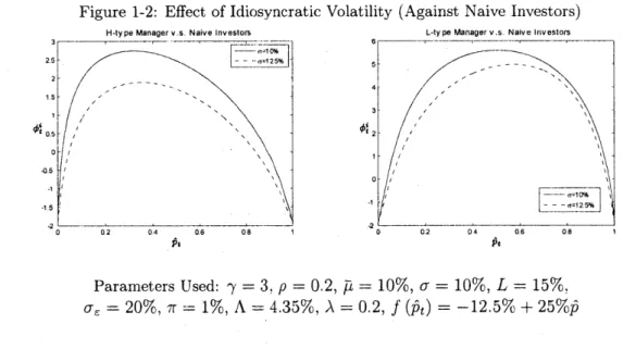
is sufficiently low to avoid being nailed down as a unskilled manager.

Figure 1-2: Effect of Idiosyncratic Volatility (Against Naive Investors)

H-ty pe Manager v.s. Naive Investors L-ty pe Manager v.s. Naive Investors

2.55 - -- '!225 4- -1. -- - - - -4 O0.5 2 - -0 --0.5 -1.5 - a=1 2.5% 0 0.2 0'4 0.6 0.8 1 0 0.2 0.4 0.6 08 1 Pt Pt Parameters Used: -y = 3. p = 0.2, p! = 10%, o = 10%, L = 15%, 0-, = 20%, 7r = 1%, A = 4.35%, A = 0.2,

f

(Pt) = -- 12.5% + 25%P

Fig 1.2 demonstrates the effect of idiosyncratic risk a of the pre-specified strategy on the optimal latent risk exposure taken by H-type and L-type managers. Higher idiosyncratic risk u increases the noise level in the fund return. As a result, the sensitivity of updating

3 decreases at all levels of reputation

Pt.

This creates less incentive for managers to boost return through taking latent risk, which leads to lower levels of optimal latent risk exposure. As a increases from 10% to 12.5%, we see that both types of managers lower their latent risk exposures.