The knowledge content of statistical data

(1)

PSYCHOMETRIKA--VOL. 62, NO. 1, 133-161 MARCH 1997

T H E K N O W L E D G E C O N T E N T O F S T A T I S T I C A L D A T A LUCIEN PREUSS

FELDEGGSTRASSE 74, CH 8008 ZI]RICH, SWITZERLAND HELMUT VORKAUF

UNIVERSITY OF FRIBOURG AND SWISS FEDERAL OFFICE OF PUBLIC HEALTH An information-theoretic framework is used to analyze the knowledge content in multivariate cross classified data. Several related measures based directly on the information concept are proposed: the knowledge content (S) of a cross classification, its terseness (Zeta), and the separability (Gammax) of one variable, given all others. Exemplary applications are presented which illustrate the solutions obtained where classical analysis is unsatisfactory, such as optimal grouping, the analysis of very skew tables, or the interpretation of well-known paradoxes. Further, the separability suggests a solution for the classic problem of inductive inference which is independent of sample size.

Key words: cross classification, association, information, entropy, inference, paradox, significance.

1. Introduction

In a fundamental p a p e r Lindley and Novick (1981) consider the basic p r o b l e m of inference and analyze Simpson's well-known but still disquieting p a r a d o x about inference (cf. Exemplary Applications, section 7.1), stating that " T h e p r o b l e m addressed (in this paper) is that of providing a formal framework within which related problems can system- atically be resolved."

Consider the fundamental nature of Simpson's paradox, and of several other simple, yet seemingly untractable problems of inference, such as Lindley's (1957) paradox, the search for an optimal n u m b e r of control cases (Fleiss, 1981), the search for an optimal formation of classes ( G o o d m a n & Kruskal, 1954), and Finley's t o r n a d o prediction (Good- m a n & Kruskal, 1959). Noting that most of them involve the use of a m e a s u r e of association, the following declaration of intent remains as valid today as it was when G o o d m a n and Kruskal stated it 40 years ago in their classic review "Measures of Association for Cross Classifications" or when it was reprinted 25 years later in 1979: " O u r major theme is that the measures of association used by an empirical investigator should not be blindly c h o s e n . . . , but should be constructed in a m a n n e r having operational meaning within the context of the particular p r o b l e m " (preface).

T h e present p a p e r revisits the fundamental inferential problems in this spirit and proposes an a p p r o a c h p r o m p t e d by the statement: " T o obtain a m e a s u r e of association o n e must s h a r p e n the definition of association, and this m e a n s that of the m a n y vague intuitive notions of the concept some must be d r o p p e d . " ( G o o d m a n & Kruskal, 1954, p. 742)

T h e statistical dependances found in a cross classification represent knowledge de- Lucien Preuss gratefully acknowledges the support of the Swiss National Science Foundation (grant 21- 25'757.88) which provided the initial impetus for this work. Also, we owe more than the usual thanks to the Editor, Shizuhiko Nishisato, whose relentless demands for clarity resulted in quite a few improvements.

Requests for reprints should be sent to Helmut Vorkauf, Swiss Federal Office of Public Health, Hessstrasse 27, CH 3097 Liebefeld/Bern, SWITZERLAND.

(2)

rived from past experience and can be used for a transfer of information between the variables. One must maintain a sharp distinction, however, between the description of dependance, generally expressed in terms of probabilities, and an evaluation of the dependance's strength, expressed as an amount of information about a dependent variable that can be derived from an independent one. Consider a 2 x 2 table with four identical frequencies: the probability to guess the value of one variable given the other has the sizeable value ½, although there is clearly no association. Measures of association should reflect the amount of information that the knowledge of one variable provides about the other. Note that the probability to get certain results is not such a measure of association, but that Shannon's (1948) concept of information is, It defines information as the reduction of uncertainty or entropy from a distribution before an event to a distribution after it, irrespective of whether the event reveals the result of a single observation or of a whole set. This concept can be directly applied to a cross classification to evaluate the average information "w" obtained when passing from a mere knowledge of the margins to the unambiguous identification of a single event, and, perhaps more importantly, to distinguish two distinct parts of this information:

• The global restriction imposed on the distribution when the disclosure of a cross classification replaces the expected distribution with the observed frequencies, called the static content "S" of the cross classification, and

• The remainder (w - S), which represents the contribution of an actual observation, given the cross classification. This remainder is equal to the joint entropy of the cross classification.

Further, Shannon's concept can be used to derive a directed and normalized measure of dissimilarity for comparing any number of distributions for inductive inference. This dissimilarity measure, called "separability" and defined later, satisfies the following conditions:

• It is invariant when all frequencies are multiplied by the same factor. This is trivially necessary for a comparison between theoretical distributions for which only relative frequencies are defined, but it must also hold for observed distributions, because such distributions will not become more dissimilar when their frequencies are doubled or tripled.

• It is applicable to distributions which are not mutually absolutely continuous; this is necessary both for reasons of continuity and for generality.

• Its interpretation does not depend on a discontinuous parameter such as the degrees of freedom of a contingency table. Karl Pearson was apparently never quite satisfied with the accepted method of determining the number of degrees of freedom of a contingency table (Kendall, 1943, p. 305), possibly because an arbitrarily small alter- ation of the data allows one to inflate this number at will through the addition of cells with near-vanishing expected frequencies outside the original frame of the table. It is unsatisfactory in theory and poses problems in practice to avoid this problem by imposing some arbitrary lower bound for all expected frequencies.

This dissimilarity measure has been suggested in the past as a measure of dependency (S~irndal, 1974; Press, Flannery, Teukolsky & Vetterling, 1989). In order to capitalize on the power and simplicity of the information approach, the separability of distributions must be analyzed in some depth and complemented with related parameters. The use of the following three measures then greatly simplifies the analysis of dependence between any number of variables and yields satisfactory and coherent solutions for several vexing problems and seemingly untractable paradoxes:

(3)

L U C I E N PREUSS A N D H E L M U T V O R K A U F 135 • The static content S of a multidimensional table to evaluate the information provided when the expected frequencies are replaced by observed frequencies. Monitoring the static content is essential when there is an abundance of variables, some of which must be removed to get a better overview (sec. 7.2). It also allows to compare the useful content of very skewed or otherwise unusual cross classifications with that of more familiar ones (sec. 7.4).

• The "terseness" of a multidimensional frequency table to measure the efficiency of the grid used to represent the observations. It is defined as the ratio of the maximal information that can be extracted from the cross classification through an appropriate input, to the amount of information that must be invested for the purpose. The terseness is needed to assess the desirability of deliberate modifications of the representation, as in searching for an optimal grouping (sec. 7.5), or when reducing the number of variables (sec. 7.1, 7.2).

• The separability to measure the dependence of any subset of variables on the complementary subset. It allows a systematic analysis of dependence in multidimensional cross classifications (sec. 7.2) and a comparison between widely different ones (sec. 7.4). Further, it is an absolute measure for the inhomogeneity of an ensemble of distributions (sec. 7.5) and, last not least, for the adequacy of a hypothesis (sec. 6.1). The first two measures pertain to the cross classification as a whole and are symmetric in all its variables, whilst the last is a directed measure which characterizes a single variable, or a subset of variables. None depends on the number of observations, but their dependability (hence that of any conclusion based on them) clearly does. A theoretical derivation of their asymptotic standard errors seems desirable, but was not attempted here.

2. Entropy

The concept of entropy used in information theory (Khinchin, 1957; Schmitt, 1969; Shannon, 1948) will be sketched only very briefly. The entropy of a distribution is a quantitative measure for the uncertainty of its outcome. This uncertainty does not depend on any single probability, but on the homogeneity of the entire distribution. If the distribution encompasses only a few and widely different probabilities, the outcomes with larger probabilities will occur overwhelmingly often, and the uncertainty of the distribution becomes correspondingly low. Conversely, a distribution of events with nearly equal probabilities has a highly uncertain outcome; therefore, much information is delivered when an outcome becomes known.

The entropy H of a distribution Pl, P2 . . . Pi, • • • , P k with k distinct elements is: H [ p l , P2, P3 . . . . , Pk] = ~ q~(Pl), ( l a ) or, when using frequencies a i instead of probabilities Pi:

1

U [ a , , a 2 , a3 . . . . , ak] = ~ ~ q~(ai) + In N ( l b ) where

I

- a " In (a) if a > 0

q~(a) = 0 i f a = 0 and N = ~] ai.

For a cross classification represented by a three-dimensional table with marginal sums

(4)

c

eij~ = ~ l~ ai..aj.a..k.

(2) AS entropies depend on relative frequencies only (see (la)), the factor c can be chosen arbitrarily, so that we can, without loss of generality, normalize the sum of all frequencies to 1 through a division by N. The entropy w of the expected or a priori distribution is the sum of the entropies of its marginal distributions, and this is the maximal uncertainty obtainable:

w = H(X) + H(Y) + H(Z)

(3)

= ~

~, q~(ai..)+

~ q~(aj.)+ ~ q~(a..~) + 3 I N N .

Once the actual or a posteriori frequencies

aij k

of a cross classification are known, its entropy is given by

1

u = ~ ~ ~#(aijk) +

In N. (4) This is called the joint entropy H(X, Y, Z) of the cross classification. Although three dimensions were used for convenience, the above equations extend to more dimensions in a straightforward manner.

3. Information

Information is a reduction of uncertainty caused by an event that replaces a prior distribution by a posterior distribution. Thus, if the result of an event is either not unique or cannot be determined with certainty, a residual posterior entropy remains and the information delivered by the event will be less than the full entropy of the a priori distribution. This includes the limiting case when nothing happens: the original distribution remains in force, and no information is generated. In communication theory, the existence of a residual entropy in any data after an event (e.g., the transmission of a message) nearly always implies a loss, for instance due to the noise in the channel. In contrast, statistics is the art of willfully introducing uncertainties, grouping similar but unequal results into classes with sometimes sizeable entropies, in order to gain a terser and more easily inter- preted image of the observed phenomena. The extent of the grouping is a fundamental, if often neglected, question. Grouping is usually performed casually, without guidance from statistical theory.

A cross classification is a static representation of knowledge, derived from past observations and stored as more or less reliable linkages of the type: "If something is living, grey, and huge, then it is probably an elephant" or " A person inoculated against cholera is probably not befallen by cholera". Knowledge reflects the awareness of such stochastic links, and the ensemble of all links between the variables of a cross classification will be considered as its "knowledge content", a concept distinct from that of information because it is static while information exists only in status nascendi, when passing from one state to another.

The analysis of cross classifications then raises the following questions:

• How much information is contained in a cross classification, or, more precisely, how much information is conveyed when one is informed of its content?

• How thoroughly can the knowledge in a cross classification be exploited?

(5)

LUCIEN PREUSS AND HELMUT VORKAUF 137 depend on the ensemble of all others? How much can be inferred about the dependent variables without looking at them, merely from inspecting the independent variables?

All three questions are readily answered in terms of information, through the definition of three fundamental coeffcients that characterize a cross classification:

• S, its knowledge content • ~, its terseness (Zeta)

• 7xY .. . . the separability (Gamma) of variables X, Y, . . . . given all others.

These coefficients will now be presented in some detail, and the solutions they provide for a number of unsolved problems will be examined.

4. Static Content of a Cross Classification

Given a cross classification with any number of variables, it is natural to ask for an evaluation of the amount of information generated by its disclosure, when passing from a mere knowledge of its margins to that of joint frequencies.

When only the marginal distributions are known, one must assume the distribution that exhibits the greatest possible uncertainty, or entropy, given the constraints exerted by the margins. This choice of the most non-committal prior distribution can be justified by Jaynes' (1978) principle of maximum entropy (Maxent). In other words, the entropy before the disclosure of the cross classification equals the joint entropy w of the expected distribution.

By definition, the entropy after the disclosure of a cross classification is equal to its joint entropy u, hence the information gain or uncertainty reduction, obtained through a

knowledge of the cross classification, is:

S = w - u. (5a)

This is the amount of information delivered when an "expected" distribution is replaced by a set of observed frequencies which reflect the linkages between the variables. As this information is delivered once and for all by the cross classification and does not depend on further input, it will be called the static c o n t e n t of the cross classification. According to (3) and (4) it can be calculated as follows for D = 3 variables:

1[

]

S = w - u = ~ ~2~ ~p(ac.) + ~'~ q~(aj.) + ~ , q)(a..~) - ~', ~p(aqk) + ( D - 1) l n N .

(Sb)

It is easy to generalize this to any number D of dimensions.

Like any measure of information, S depends on the base of the logarithms; natural logarithms will be used in this paper. Because S measures the difference in information between expected and observed distribution, it is closely related to what Fisher (1922) called "the departure of the sample from expectation". To evaluate this departure, Fisher (1922, 1956) and others (Edwards, 1972, 190-197; Wilks, 1935; Woolf, 1957) advocated "L", the logarithm of the likelihood ratio, which in two dimensions is identical to the product of the static content with the number N of observations. However, this inclusion of N into the measure obscures the essential distinction between:

• the dissimilarity between the expected and the observed distribution, and

(6)

A

9

1 Table 4.0

B

2

900

7

680

745

700

Clearly, dissimilarity does not depend on the number of observations, because multiplying all frequencies by a factor, even a large factor, does not change the distributions and will not make them more dissimilar. Hence a sharp distinction must be maintained between the magnitude of a dissimilarity and the dependability with which this magnitude is determined.

This is illustrated by Tables 4.0 A and B. Table 4.0 A displays a large dissimilarity between the expected and the observed frequency distribution, but the magnitude of this dissimilarity is not known precisely because few events have been observed and the knowledge they provide is correspondingly uncertain. Conversely, Table 4.0 B exhibits only a small dissimilarity which can, however, be assessed quite dependably. Yet the )(2 of both tables is 8.9. The necessary distinction between the magnitude of a dissimilarity and the dependability with which it can be established requires the use of the static content as a measure of the deviation of a sample from expectation instead of the logarithm of the likelihood ratio or t 2 . Using the static content also avoids the thorny subject of determining the degrees of freedom.

It may be worthwhile to remember that Pearson's )(2 is an approximation to twice the log likelihood ratio L that holds for sufficiently small deviations from expectation and sufficiently large cell frequencies: "in those cases, therefore, when 12 is a valid measure of the departure of the sample from expectation, it is equal to 2L; in other cases the approximation fails and L itself must be used" (Fisher, 1922, p. 358). Fisher then notes that when 12 approximates 2L closely enough to be valid, its practical value lies in the avail- ability of a general formula for its distribution, an essential asset before the advent of computers.

4.1 Additivity Theorem

An essential feature of the static content is its additivity when a multidimensional cross classification C1..Q (spanned by the variables X1, X2, • .. X L . . . . X Q ) is broken down into two complementary tables:

• a cross classification C1..L of L dimensions (1 < L < Q), for which the remaining dimensions are suppressed by summation, plus

• a cross classification CO;L),L+I . . . . Q obtained by removing all mutual dependences between dimensions 1 . . L. The removal is effected by replacing variables 1 . . L by their direct product, i.e. by a single variable each value of which represents a combination of values of X 1, X 2 . . . X L. (this will be called "uncoupling").

Let ul..O be the joint entropy of C1..a, and wl. ,a its expected entropy, the entropy of the distribution expected from its margins, and $1..a its static content. Similarly, u, w, and S with subscripts " 1 . . L" and "(1; L), L + 1 , . . . Q" indicate the corresponding measures for the two other cross classifications. The entropies of the margins of the original cross classification C1..Q are designated by H(X1), H(X2) . . . H(XQ).

(7)

L U C I E N PREUSS A N D H E L M U T V O R K A U F

Table 4.2.1" Data calculated from Fleiss (1981 )

(Fleiss' table reports proportions only)

139

New York

London

iiiiiiiiii i i

Age Grou p

Normal

Schizophrenic

Normal

Schizophrenic

I

24

81

71

34 II

74

118

69

63

82

52 III

105

93

wl..L = wL.o - [H(XL +1) + H(XL +2) + " " + H(X0)]. (6a) T h e expected entropy of the cross classification CO;L),L+a .... Q is

W(,;r),r +1 . . . . Q = Ul..L + [H(XL+I) + H(XL+2) + ' ' " + H(XQ)]. (6b) Because uncoupling any number of variables does not change the joint entropy of a cross classification, one has

U ( 1 ; L ) , L + 1 . . . . Q = U l . . Q .

This, together with (6a), (6b), and the definition S~ = w k - u k for any index k (simple or compound), leads to:

S 1 . . L -~" S ( t ; L ) , L + 1 . . . . Q ~--- W(1, .L) - - U ( I . . L ) -~ W ( 1 ; L ) , L + 1 , . . Q - - U ( 1 ; L ) , L + 1 . . . . Q

= w1.,Q - [H(XL + 1) + H(XL +2) + " ' " + H ( X o ) ] - ul..L + Ul..L + [H(XL +,) + H(XL + z) + " ' " + H ( X o ) ] - ul.,Q

= W l , .Q - - U l . . Q

~- S l . . Q ,

which proves the decomposition of the static content of C1..Q into the sum of the static contents of C1, 2 .... L and of CO;L),L+I . . . . Q, q.e.d.

McGill (1954) and Fano (1961, 57-58) suggested a measure of mutual information defined in a space with an arbitrary number of variables, which can be expanded into a sum of similar mutual informations defined in subspaces of that space. It can, however, be either positive or negative and is difficult to interpret.

4.2 A d d i t i v i t y T h e o r e m : N u m e r i c a l Illustration

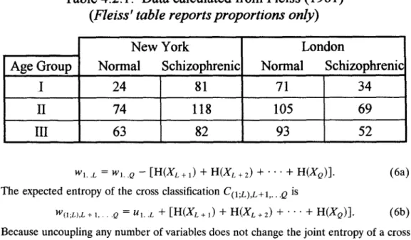
The additivity theorem will be illustrated by a three-way classification shown in Table 4.2.1, which presents the number of patients diagnosed as schizophrenic by resident hos- pital psychiatrists in New York and London, broken down by age.

T h e )(2 of this 2 × 2 × 3 table amounts to X 2 = 75.98, its static content is S = 0.0453. It seems desirable to compare the static contents which accrue in two complementary situations:

• When considering only the dependence between the Diagnosis and the Town where it originated, without regard to the patients' A g e . The corresponding table is obtained

(8)

Table 4.2.2: Age summed out

N e w Y o r k

London

Normal

161

269 Schizophrenic

281 ...

155

by summing out the Age, which results in the 2 x 2 Table 4.2.2. For this table one has g2Town,Diagnosis = 63.19, the corresponding STown,Diagnosi s = 0.0369.

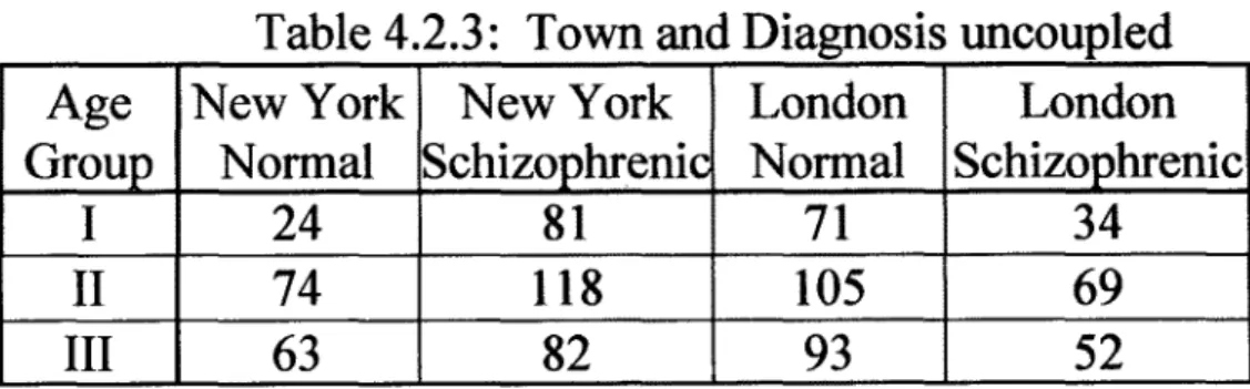
• When neglecting the dependence between the Diagnosis and the Town where it originated. To this end one must uncouple the variables Town and Diagnosis, which yields the 3 x 4 Table 4.2.3, (superficially identical to Table 4.2.1 which was 3 rows by 2 x 2 columns, whereas Table 4.2.3 is restructured as 3 rows by 4 columns) showing the dependence between Age and the two other variables when these are made independent of each other. H e r e , X~(Town;Diagnosis),Age is reduced to 13.63, S(Town;Diagnosis),Ag e to 0.0084.

The listed values show that for a mere dependence between Town and Diagnosis the static content is about 4.4 times larger than for a dependence between Age and (Diagno- sis + Town), neglecting any dependence between the latter two. This provides essential information about the relative importance of the different factors involved. Adding both calculated values of S gives the static content of the origina ! three-dimensional table, as required by the additivity theorem:

S T . . . . Diagnosis + S(Town;Diagnosis),Age = STown,Diagnosis,Age = 0 . 0 3 6 9 + 0.0084 = 0 . 0 4 5 3 .

The additivity guarantees that these values of S can be meaningfully compared, which shows that by disregarding the interaction between Town and Diagnosis one discards more than 80% of the static content of the survey. Conversely, an exclusive consideration of this interaction alone results in a loss of less than 20% of the original content. This comparison provides a vivid picture of the actual dependence.

The corresponding values of X 2 have been added for completeness, and they show that in this well-behaved case X 2 deviates only slightly from additivity:

2 2 2

XTown,Diagnosis q- ~((Town;Diagnosis),Age XTown,Diagnosis,Age, i.e., 63.19 + 13.63 = 76.82 ~ 75.98.

This is not always true, however, and large deviations from additivity can occur.

Table 4.2.3: Town and Diagnosis uncoupled

Age

Group

I

II

New York

Normal

24

74 New York

Schizop~enic

81

118 London

Normal

71

105 III

63

82

93 London

Schizophrenic

34

69

52

(9)

LUCIEN PREUSS AND HELMUT VORKAUF 141 5. Efficiency, or Terseness, of Knowledge in a Cross Classification

Passing from an expected distribution to the observed cross classification reduces the entropy of the considered ensemble from w to u and yields the information S = w - u. The entropy u left over reflects the uncertainty that remains because the process specifies an entire distribution, without pointing at any cell in particular. The remnant is equal to the average amount of information needed for addressing a cell. Now, one often wishes to use the linkages defined by non-empty cells to transfer information from one or several variables which are viewed as independent to a variable which is viewed as dependent. For each such transfer one must access the appropriate cell, which requires an input of information at least equal to the joint entropy u. The economy of such a transfer is a direct measure of usefulness of the knowledge embodied in the cross classification.

Remarkably, neither the total input u nor the total output--which will be called the variety "rY' of the cross classification--depends on which variable is chosen as input, provided the input is entered in a way to generate the maximum possible output of information, as shown below. Therefore the ratio v/u of output to input is a parameter of the cross classification, and indicates quantitatively how efficiently it can be used for the retrieval of a ' single variable value. This ratio shall be called the terseness of the cross classification and designated by the Greek letter ff (Zeta). It is the efficiency of the cross classification as a repository of knowledge, namely the information that can be extracted from it (e.g., as an inference) relative to that which must be entered for the purpose (e.g., as a premise).

For the sake of simplicity, u and v will be determined for a cross classification with just four variables X, Y, Z, and T. The symmetry of the resulting expressions makes it easy to extend the formulation to an arbitrary number of variables. The minimal necessary input for the selection of a cell is identical to the joint entropy u of the cross classification, as shown in the following identification sequence, at each stage of which all residual entropy is removed from the current coordinate. Its steps are:

• An unconditional determination of X, leaving no residual uncertainty about X. • The choice of Y conditional on the value of X already chosen, resulting in no residual

uncertainty with regard to Y or X.

• The choice of Z conditional on the chosen values of X and Y, leaving no residual uncertainty with regard to Z, ¥, or X.

• The choice of T conditional on the chosen values of all other variables. This final step leaves no residual uncertainty at all.

Summing up the entropy reductions at all four steps shows that the total information I necessary for the identification of a cell is equal to the joint entropy u (or H(XYZT)) of the cross classification, as expected:

I = H(X) + H(YIX) + H(Z1XY) + H ( T I X Y Z ) = u. (7) It remains to determine the amount v of information recuperated in the course of this sequence. To identify a cell, the variables X, Y, Z, and T must be assigned definite values. Given the constraints imposed by the cross classification, these assignments are generally not mutually independent. Suppose that X is determined first. This choice reduces the entropy by AHx, where

AHx = H ( Y Z T ) - H ( Y Z T I X ) -- I(YZT; X). (8a) The identity on the right side of (8a) is but a particular form of a standard identity of communication theory, where I(YZT; X ) is called "mutual information" between X and the three-dimensional variable YZT, or "information transmitted" between X and YZT.

(10)

Being an average, this amount does not depend on the actual value of X. Due to the symmetric nature of I ( Y Z T ; X ) , equation (8a) can be written in the following form which is more convenient here:

AHx = I(X; Y Z T ) = H(X) - H ( X I Y Z T ) . (8b) Thereafter, when a particular value of Y is given, the entropy reduction of Z and T can be expressed as

h n x y = H ( Z T I X ) - H ( Z T I X Y ) = I(ZT; YIX), (9a)

o r

hHxy = I(Y; Z T I X ) = H(YIX) - H ( Y I Z T X ) . (9b) Finally, when a particular value for Z is chosen among those still allowed for it, this selection reduces the entropy of the last remaining variable T by the amount

hHxrz = H(TIXY) - H(TIXYZ) = I(T; ZIXY), (10a)

o r

AHxvz

=

I(Z; TIXI0 = H(ZIXY) - H(ZITXY).

(10b)

The addition of (8b), (9b) and (10b), yields the sum v of all entropy reductions that the cross classification imposes on the output, given the required input u:

v = AHX + AHxr + AHxvz ( l l a )

= H(X) + H(YIX) +

H(ZIXY)

- H ( X I Y Z T ) - H ( Y I Z T X ) - H(ZITXY).

Equation (11a) shows the restrictions that the cross classification imposes on the choice of the coordinates, when the input values are entered in the chosen order (to wit: X, Y, Z). One can easily show, however, that v is independent of this order. Adding and subtracting the additional term H(T~'YZ) on the right-hand side of (11a), yields

v = u - H ( X I Y Z T ) - H ( Y I Z T X ) - H(ZITXY) - H(TIXYZ), ( l i b ) where

u = H(X) +

H(YIX) + H(ZIXY)

+ H(TtXYZ) 1

= ~ • q~(axyz,) + In N

(12)

is the joint entropy H(X, Y, Z, T) of the cross classification, and symmetric in all variables. As the remaining four terms on the right-hand side of (11b) taken together are symmetric too, v is symmetric in all variables, and therefore independent of the chosen sequence.

Extending (11b) and (12) to D dimensions X1, X2, X3 . . . X D yields

(13) with D v = H(X1, X2, X 3 , . . . , XD) -- ~ H ( X i l X 1 , . . . , X i - 1 , X i + l , . . . , XD) i=1 u = H(X,, X2, X s . . . XD). (14)

(11)

LUCIEN PREUSSAND HELMUT VORKAUF 143 Thus, the terseness of a cross classification with an arbitrary number D of entries becomes

v Z n ( s i l s , . . . .

, x i _ l , x , + l . . . xD)

= - = 1 - - . ( 1 5 )

u H ( X I , X z , X 3 , . . . , X D ) One easily sees that

D

o ~ ~ H(X,-Ix1 . . . .

,x+_~,X++~ . . . . ,Xo) ~- H(X1,X2, X3 . . . . ,Xo),

i=l

(15a)

with equality on the left if and only if any D - 1 variables uniquely determine the remaining one, and with equality on the right if and only if all variables are statistically independent, from which it follows that 0 -< ~ -< 1. Since the terseness is a quotient of two logarithms, it provides an absolute measure, independent of the logarithms' base. Rajski (1963) suggested the quotient of transinformation and joint entropy as a replacement for the correlation coetficient in a two-way table; this equals Zeta in two dimensions, but differs in more than two dimensions, where it may even become negative (Rajski, 1961).

Thus a cross classification yields two distinct pieces of information, namely: • the static content S determined by (5b), and

• the variety v = ~" u determined by (13).

Adding S and v, and indicating by Y~ Haverag e the sum of the average entropies of all rows, columns, etcetera in a mu--rtidimensional cross classification (each average being conditional on all variables save one, as in (llb)), one gets the entropy reduction:

g = s + ~ ' u = ( w - u ) + ( u - ~ H

. . . ge) = w - E Uaverage • (16) This is the total amount of information gained from a cross classification in the course of a transition from total ignorance to the unambiguous identification of one particular event. Overall, this transition delivers the amount of information equal to w, less the useless entropy reductions due to a distinction between events that are mutually "aligned" along rows, columns, lines, etc. of the cross classification. Events which are mutually aligned differ only by a single feature, and the selection of one such event cannot yield any other output than the very information that was entered in order to select it; abandoning this distinction without a difference entails a loss equal to the sum subtracted from w on the right-hand side of (16). The static content S plus the product flu of terseness and joint entropy represent the total K of all information that can be obtained from a cross classification, given an appropriate input. K will be called the overall knowledge content of a cross classification.

In two dimensions both parentheses in equation (16) are numerically equal. In other words, the amount of information S obtained when one is informed of the content of a cross classification is equal to the largest that can be obtained from it thereafter through an appropriate input. However, this equality holds only in two dimensions, and created some confusion in the past. It led to the definition of a symmetric uncertainty coefficient

2S/w

occasionally cited in the literature (Brown, 1975; Press et al., 1989) and implemented in statistics packages (SAS, SPSS, SYSTAT). 1 This coefficient is unsatisfactory because it lacks a straightforward interpretation. Also, it does not readily extend to more than two t For information regarding SAS Version 6 contact SAS Institute, Inc., SAS Campus Drive, Cary NC, 27513-2414 (Phone: 1-919-677-8000. Web site: www.sas.com). For information regarding SPSS/PC + Advanced Statistics or SYSTAT contact SPSS, Inc., 444 North Michigan Avenue, Chicago, IL 60611 (Phone: 1-800-543- 2185. Web site: www.spss.com).

(12)

variables and must hence be normalized artificially by including the number of variables in its definition; this cannot be achieved, however, without introducing inconsistency when the frequencies in some cells tend to zero.

6. Separability of a Variable

When analyzing a cross classification, the primary interest often lies neither in S nor in ~, but in the amount of information that the cross classification can usefully transfer from one variable, or from one set of variables, to another. Thus, it may be desirable to determine, for example, how much information about the future health state of a person can be inferred from his or her observable present vaccination status, using the statistical knowledge contained in a table of past results of this type of vaccination.

The term "dependence" is traditionally used for the strength of such inferences (also called "associations") and will be retained here. It should b e u n d e r s t o o d that it need not imply any actual relation from cause to effect (Jaynes, 1989), although the well-entrenched term "dependence" will often be applied here, even if common usage suggests a causal interpretation.

As a rule one is not so much interested in the absolute amount of transferred information than in its relative extent compared to what might have been obtained through a direct observation of the variable of interest (see Salk vaccine example, Table 7.4.1). Given a cross classification, a fraction of the information that would be gained by directly ob- serving the independent variable can also be gathered indirectly through an observation of the dependent variable. This fraction provides a readily interpretable measure of the extent to which the dependent variable determines the independent one. It is a dimen- sionless, normalized measure of the efficiency of the directed inference from a variable, or a set of variables, to the complementary one. Because it evaluates the ease with which values of a variable can be distinguished through an exclusive observation of the complementary variable, it will be called the separability 3'x of X, when X is viewed as the independent variable.

The efficiency of an indirect observation will now be derived in more detail. As this involves only two variables, independent and dependent (observed), the following considerations can be restricted to a two dimensional cross classification spanned by these two (possibly multidimensional) variables. One may further suppose that the independent variable represents entities, whilst the actually observed variable identifies features at- tached to the same. The ratio of the indirect information to the direct one then measures how efficiently entities can be distinguished from each other through the mere observation of their features.

Let the frequency of a simultaneous occurrence o f x i a n d y / b e aij, and call the sum of all frequencies N, that is, N = E aij. If an event x i occurs and is observed directly, no residual uncertainty is left over after the event; hence the generated information equals the original entropy of X, that is, the entropy of the marginal row:

1

H(X) = ~ ~ ¢(ai.) + In N. (17)

Suppose now that variable X cannot be observed directly, but only through an observation of variable Y which has the value yj. As a result of this observation, the distribution of X shrinks from that of the marginal row to that of row j. The former has the entropy H(X), and the latter the smaller entropy H(X~vj). It follows that, on average, each observation of Y reduces the original entropy H(X) to a posterior value H(XIIO which is the average entropy of X given Y. For the calculation of this average, the entropy of each row

(13)

LUCIEN PREUSS AND HELMUT VORKAUF 145 must be weighted according to its frequency a.j. Subtracting the average residual entropy of X after an observation of Y from the entropy of X before this observation yields the information I(X; Y) about X r e t u r n e d - - o n average--by an observation of Y:

I = H(X) - H(XIY). (18)

This is the "transinformation" of communication theory. If one divides it by the amount of information H(X) that could in principle have been gathered through a direct observation of X, one obtains the fraction of the total information about X obtainable through an observation of Y, which will be called the separability ~/x of X given Y:

H(X) - H(XtY)

Yx = H(X) (19a)

The separability "/x is normalized to one and remains constant when all frequencies are multiplied by the same factor. The separability ~/x applies to an arbitrarily large set of distributions Yi, one distribution per each particular value of X, and measures the ease of distinguishing (or separating) the distributions through the mere observation of Y. In general the separability thus determines the heterogeneity of a set of distributions. I f X is a dichotomous variable, a difference between two distributions is measured as in the Kolmogorov-Smirnov test or with Rajski's (1961) dx, y. The latter evaluates a distance between the margins of a two-entry table and satisfies the metric axioms. Formally, it is closely related to the terseness in two dimensions and to the separability, through the equations dx, Y = 1 - ~ and (2 - dx, y)/(1 - d x y ) = 1/Vx + 1/3~r, but its rationale is different. In particular, the distance dx, Y is limited to two distributions and does not evaluate their dissimilarity because it remains constant under all permutations of the frequencies in either distribution.

In analogy to definition (19a), the separability 3'Y of Y given X equals the fraction of the total information about Y obtainable through an observation of X:

H(Y) - H(Y[X)

Yr = H(Y) (19b)

The separability ranges from zero to one, inclusive, and is independent of the base chosen for the logarithms used when calculating the entropies. Note that the range from 0 to 1 of both terseness and separability should not be used as in the interpretation of correlation coefficients. Whereas a correlation of 0.10 may express less than remarkable association, a terseness or a separability of that magnitude should be considered striking, even 0.01 is nothing to be discarded easily. Values of ~/or ~ above 0.10 indicate an exceptionally strong association.

The separability has been repeatedly suggested--under various names like "asym- metric uncertainty coefficient"--as a measure of association (e.g. Press et al, 1989), often on the ground of its belonging to a class of measures which evaluate "the relative reduction in uncertainty about Y from getting to know X" (Sfirndal 1974). Actually, it is the only measure which fully satisfies this definition when one interprets uncertainty as lack of information. Further grounds for its importance lie in its close relationship with the information S obtained "from getting to know the cross classification" (to paraphrase the above definition) and also with the terseness ft.

6.1 Model for Inductive Inference based on the Separability

Consider a two-column table where the column widths represent time intervals. The table contains events generated by a hypothetical parent distribution of the marginal

(14)

Table 6.1.1: Minimum necessary change for some artificial data

H

D

Y

0.64

75 Yy

0.32

23 y

0.04

2 J = y(D,QN)-(NQ/ND)

N=25 =50 =75 5 21 37 17 25 33 3 4 5

Columns QN

=88 =100 =125 =150 =175 =200 45.3 53 69 85 101 117 37.2 41 49 57 65 73 5.5 6 7 8 9 10 . 0 5 2 7 9 . 0 4 1 8 8 . 0 3 9 8 3 . 0 3 9 7 0 . 0 3 9 7 6 . 0 4 0 4 9 . 0 4 1 6 0 . 0 4 2 9 2 . 0 4 4 3 8

column. Each row represents a possible outcome. If the boundary between the two columns corresponds to the present time, the table can be viewed as a yet incomplete cross classification that compares the left column of ND observed data with hypothetical future data that wait to be collected in the right column. Because empirical observations may never be disavowed, any conceivable future data set that one wishes to compare with the hypothesis must include the observations already made. The essential consequence of a divergence between the assumed parent distribution and the data already sampled can be verified empirically and is to be found in the occurrence of future outcomes not consistent with the most probable distribution to date (that of the sample in the left column), but needed to compensate the divergence between the observed data and the assumed hypothesis. This set Q, composed of NO virtual events, is not uniquely determined: there may be either few events strongly separated from the observed set, or many events weakly separated from it. By definition, past and future sets stem from the same parent universe, hence their separability Yoa should be small if the hypothesis is to be plausible. Because the ratio NQ/N D evaluates the relative weight of the unwarranted virtual events, the product J = (NQ/ND) • ]/DQ of the separability with this ratio is a measure of the distortion introduced in order to turn the observed set into part and parcel of a most probable set under the hypothesis. The minimum of J will be called the tw/st and designated by r. It is a lower bound for the arbitrariness required to bring the full set of events into line with the hypothesis and evaluates the smallest departure from the distribution of the sample that must be imposed on future events to satisfy the hypothesis. The twist is a natural measure, and hopefully a valid quantitative estimate, for the distortion which the assumption of the hypothesis imposes on the future events, given the data.

These considerations suggest the following procedure, illustrated by the artificial data of Table 6.1.1, where column D represents the observed set of data, column H the proportions expected under a hypothesis (a binomial distribution withp = 0.8 in this exam- pie), and the columns QN represent sets of virtual observations that are so calculated that each column QN combined with column D forms a two-column table with the marginal proportions listed as in column H. (The lengthy computation is eased by a little program for the PC, available from the second author upon request). Now, N O can be made to vary continuously, and each value N O will then determine a set QN of virtual frequencies having a well-defined separability with respect to the observed set. One can then view J as a function of N O alone, for a given hypothesis and an observed set; its minimum is the twist. The virtual weights N O can vary from the lowest possible value (i.e., one not requiring negative frequencies) to one beyond which no further minimum of J exists, and can include fractional frequencies for continuity.

(15)

L U C I E N PREUSS A N D H E L M U T V O R K A U F 147

In Table 6.1.1 the twist amounts to 0.03967 and occurs for the set Qss = (45.3, 37.2, 5.5). Because the number of virtual events differs only moderately from the sample size, the denominator H(100, 88) of 7(D, Qss.)can be approximated by ln(2), so that the relation due to Fisher (1922, p. 357-58), X ~--~ 2Nv, leads to the following approximation for the twist

XD,Q

~" ~- 3'(D, Q88) ~ ~ ' (2 In 2) = 0.03916.

This shows that, when the size of the virtual complement does not differ too much from that of the sample, the twist tends to be proportional to

x2/N.

The twist, however, addresses the question, "How strongly must one distort the distribution of the data to satisfy the hypothesis.'?"; while a significance test addresses a different question, namely, "Might the sample have been generated by the hypothesis, given some reasonable variance?". (Note that the answer depends on the sample size.) The twist provides a measure of the disagreement between hypothesis and sampled data which, unlike X 2, depends only on the distribution in the sample, not on the number of observed events. This distinction heeds Fisher's (1951, p. 195) dictum, "The tests appropriate for discriminating among a group of hypothetical populations having different variance are thus quite distinct from those appropriate to a discrimination among distributions having different means". Using the twist for a comparison between several samples eliminates the difficulties due to an exclusive use of significance tests because the latter evaluate the variance that must be forced upon a hypothesis which is assumed to be absolutely exact, and which will therefore become less and less like!y when a sample gets larger without change in its distribution (except in the trivial case of complete concordance between sample and hypothesis). This not only precludes meaningful comparisons between samples of different sizes (see the example in section 6.2 which illustrates the point), it is also a hindrance when the hypothesis to be verified is not derived from some theory (as sometime available in genetics), but empirically (as is the rule in the social sciences): even if it is a very good approximation, as far as empirical formulas go, the unavoidable deviation from its (unknown) exact form will be endlessly magnified when the number of observations becomes large. Thus, due to the unavoidable asymmetry of a real die, throwing it sufficiently often will always generate an arbitrarily large significance to reject the null hypothesis of equal probability of the six sides; this, however, reveals nothing about the degree of the die's asymmetry.

The use of the twist for inductive inference can be illustrated by the data from which Bernstein (1924) concluded that the ABO blood-groups in man are determined by three alleles (A, B, and O) at a single locus (Hypothesis 1) rather than by two alleles at each of two loci (A, a; B, b) as formerly believed (Hypothesis 2). The observed frequencies and the proportions expected on each hypothesis are shown in Table 6.1.2. As the source states proportions only, the listed frequencies were reconstructed to the nearest integer from these proportions and the known sample size.

The twist necessary to compensate for the departure from the hypothesis is not only much larger for the two loci hypothesis than for the one locus hypothesis, the twist for one locus is also very small in absolute terms. The evidence in favor of Bernstein's judgment is thus overwhelming.

6.2 Lindley's Paradox, an Example

Let it be known that a certain race of rabbits has different fur patterns a, b, c, d in the proportion 4:3:2:1. One would like to know if the rabbits in A-valley belong to that race or not.

(16)

Table 6.1.2: The twist for AB0 phenotypes and one- vs two-loci

hypotheses

i

Blood group

Observed

phenotype

frequencies

Proportions assuming

one locus

!

two loci

A

212 0.4112

0.358 B

103 0.1943

0.142 AB

39 0.0911

0.142

0

148 0.3034

0.358 z, required twist:

0.00226

0.05922

A first survey of 100 rabbits resulted in the frequencies 46, 28, 18, 8 of the fur patterns (column A of Table 6.2.1). Then, without authorization, gamekeeper Fred Busybody surveyed another 100 rabbits, with frequencies 43, 29, 19, 9 (column B), producing counts 89, 57, 37, 17 for the enlarged sample of 200 rabbits (column C). As the proportions moved closer to the theoretical expectation for all fur patterns, the distribution has come closer to the expectation.

Does the enlarged survey (column C) give more support to the hypothesis than the smaller first survey (column A), in spite of its larger significance for rejection? Suppose further that survey B is followed by an endless sequence of surveys B 1, B 2 .. . . , B k . . . each of which is twice the size of the preceding one and has pattern frequencies midway between the sum of those observed to date and the hypothetical ones (allowing fractional frequencies for convenience, e.g., B 1 = {84.5, 58.5, 38.5, 18.5}, B 2 = {166.75, 117.75, 77.75,

Table 6.2.1" Two surveys and their combination

F u r

pattern

a

0.40 b

O.30 c

0.20 d

0.10 C

First survey

plus Busy-

body's data

N

p

89

0.445 Hypo-

thesis

A

First survey

B

Busybody's

additional

survey

1.633

0.408

1.838 Twist "c

0.011828

0.002948

0.006642

X 2

57

0.285

37

0.185

17

0.085 N

100

200 N

p

46

0.46

28

0.28

18

0.18

8

0.08 N

p

43

0.43

29

0.29

19

0.19

9

0.09

,, i

(17)

L U C I E N PREUSS AND H E L M U T V O R K A U F 149

37.75}). Clearly, the observed overall distribution converges asymptotically toward the hypothesis, and one can easily show that X 2 simultaneously tends to infinity with 1.125 k.

This is a simple numerical instance of Lindley's (1957) paradox, who concluded that (a significance level of) "5% in today's small sample does not mean the same as 5% in tomorrow's large one."

Survey C comes closer to the hypothesis than A, as documented by its smaller twist. In view of the history this should not be surprising: Busybody's additional sample (column B) is certainly closer by any criterion, so its addition can only move the combined sample C in the direction of the hypothesis. Yet t, 2 is increased for sample C, the twist behaves as it should. At the same time A, due to the smaller sample size, has a larger margin of error than C, and so has its twist. Thus the distribution underlying A could occasionally be closer to the hypothesis than the distribution underlying C, although this is hardly probable.

Consequently, to answer the question as to whether a distribution fits a hypothesis, we require two parameters:

• The magnitude of the disagreement between observation and hypothesis.

• The error connected with the estimate of that magnitude, or the variance about the estimated magnitude.

The disagreement is measured by the twist ~-, but we can not yet give a formula for the twist's standard error. Brown (1975) published a formula for the asymptotic standard error of 3', based on methods described by Goodman and Kruskal (1972). This calculation is not directly applicable to the twist, however, and we felt we must postpone the problem of deriving its error estimate.

7. Exemplary Applications 7.1 Simpson's Paradox

This well-known paradox (Blyth, 1972a, 1972b; Lindley & Novick, 1981; Novick, 1980; Sz6kely, 1990) is that an effect exists in both of two groups and is reversed when both groups are combined. Consider an artificial example in which the starting of a car depends on the grade of gasoline and the time of starting (see Table 7.11). High octane gas facilitates starting early in the morning as well as later in the morning, yet combining the two tables seems to indicate that low octane gas lets the car start more easily. Surely this contradiction is irritating and needs an explanation.

It is clear that cars have greater difficulty to start in the morning cold, but another aspect of the data is also clear, namely that early starters tend to use high octane gas. Thus, the choice of high octane gasoline appears inferior for starting the car, in striking contrast to the superiority of high octane gas within each time period, via the tendency of high octane gas users to start under the unfavorable condition of morning cold.

The statistician who is asked for advice might recommend high octane gas if he knows the time that a driver usually leaves home and that this time will not change; if the time of starting the car were undecided, he might recommend low octane gas, and his advice would not be as illogical as it seems at first sight. Indeed, if the strong relation between type of gas and starting time remains in force, a driver following the advice for high octane gas will more likely start in early morning, satisfying the empirical correlation between gas quality and preferred time to start the car, and as a consequence he will increase the overall frequency of unsuccessful starts. This indirect influence overpowers the superiority of high octane gas observed severally in the early morning and later. Thus, unless early starters remain early starters and late starters remain late starters irrespective of the type of gas they u s e - - o n e must indeed recommend low octane gas in order to prevent an increase of starting failures under the unfavorable conditions of early morning cold.

(18)

Table 7.1.1: Fictitious data, adapted from Novick (1980)

Motor

started

Early and Later

Combined

Prop. Yes

Early

in the morning

Low

High

Octane Octane

2

9

8

21

0.20

0.30 Later

in the morning

Low

Octane

Low

High

Octane Octane

18

7

12

3

0.60

0.70 High

Octane

Yes

20

16 No

20

24

0.50

0.40

This explains the paradox, but a simple quantitative criterion to signal the danger of the paradox occurring would be helpful. If ff decreases when a variable is eliminated from a table, this is a warning that the usefulness of the table deteriorates through the loss of a dependence essential for the interpretation of the full table. As shown in Table 7.1.2,

= 0.1056 for the full Table 7.1.1 with all three variables. It drops to 0.0037 (by a factor of 25) when one ignores Time and merely looks at the cross tabulation of Gasoline x Success, meaning that Time is of such paramount importance for the data set that its exclusion almost amounts to an "illegal" act. The only "legal" suppression would be that of the variable of primary interest, namely Success, as ~ for Time x Gasoline equals 0.1042, almost as high as for the complete three-dimensional table. Thus the main content of Table 7.1.1 is the strong association between Gasoline and Time, and ignoring this aspect of the data is punished by the baffling paradox. However, the correlation between the type of gas used and the time of starting the car--even if it is strong--is probably not a genuine dependence, as the driver who is advised to use high octane gas will scarcely change his habit of starting early or late when following the advice. Hence this advice can rest on the separate data sets for early and late starters, but a different context may lead to a different conclusion.

7.2 "The American Soldier" Revisited

A venerable data set first presented by Stouffer (1949) and used by Goodman (1978) to demonstrate the logit multiple regression approach to the analysis of dichotomous variables, and by Theil (1972) to examine the relation between logit and entropy, will be re-analyzed using the new approach.

Table 7.1.2 Terseness of all possible subtables

Variables in the cross

tabulation

Time, Gasoline, Success

Time and Gasoline

Time and Success

Gasoline and Success

Terseness

0 . 1 0 5 6

0 . 1 0 4 2

0 . 0 4 8 0

0.0037

(19)

T a b l e 7.2.1 : P r e f e r r e d l o c a t i o n b y

race, origin

a n d

present camp

Black Race Northern Southern

Ori

Present C a m p Present C a m p White Race Northern Southern Origin Origin Present C a m p Present C a m p Prefer North

North South North South North South North South 387 876 383 381 955 874 104 91

36 250 270 1712 162 510 176 869 Prefer South

Prop. North 0.915 0.778 0.587 0.182 0.855 0.632 0.371 0.095

The data in Table 7.2.1 served to study the preferred location of a training camp (Northern or Southern US state) for American soldiers of Black or White racial origin, Northern or Southern origin, stationed in a Northern or Southern camp.

An analysis of these data will raise several questions:

QI: Which factors are least informative, and may be discarded with tolerable loss of information?

AI: The least informative variables are those the removal of which causes the smallest loss of static content. They can be found by removing variables one after the other such that each removal causes the smallest loss of content achievable at that stage. Table 7.2.2 (left half) lists S and ff obtained when removing one variable from the original cross classification.

Present camp

turns out to be most disposable. Among the three remaining variables

Race

is the most unnecessary, its removal reduces the static content least, as can be seen in Table 7.2.2 (right half). After the removal of Present camp and Race, only two variables are left, so no further step is possible.

Q2: Can one make the cross classification more efficient by neglecting less informative variables?

A2: The preceding tables reveal that the initial elimination of Present Camp mar- ginally increased the terseness of the cross classification, and that the following

T a b l e 7.2.2 R e m o v e d V a r i a b l e N o n e P r e s e n t C a m p R a c e P r e f e r e n c e O r i g i n F o r s e l e c t i n g first variable to b e r e m o v e d Static T e r s e n e s s o f C o n t e n t o f R e m a i n d e r R e m a i n d e r 0 . 2 6 2 0 0 . 1 0 7 8 0 . 1 9 8 6 0.1081 0 . 1 9 6 7 0.1031 0 . 0 6 8 4 0 . 0 3 4 9 0 . 0 6 0 2 0.0301 A f t e r r e m o v i n g

Present

Camp

0 . 1 9 8 6 0.1081 0 . 1 4 3 7 0 . 1 1 5 7 0 . 0 4 8 0 0 . 0 3 5 9 0 . 0 0 2 4 0 . 0 0 1 7 Static T e r s e n e s s o f C o n t e n t o f R e m a i n d e r R e m a i n d e r

(20)

Prefer North

Prefer South

Sep. of Pref.

Terseness

Origin

South North

immll,,,,ll

959 3092

3027

958 0.2074

0.1157

Table 7.2.3

P~sent

Camp

South North

1829 2222

644 3341

0.0734

0.0404

Race

Black White

20271 2024

2268 1717

0.0034

0.0017

Q3: A3: Q4: A4:

elimination of Race increased the terseness noticeably. The process then ends for lack of variables, but in the general case it should be pursued until the terseness attains a maximum.

Which single factor influences the Preference most strongly?

This question is closely related to the preceding one, the difference being that Question 2 relates to the efficiency of the knowledge as a whole, while the present question specifically concerns the dependence of the single variable

Preference

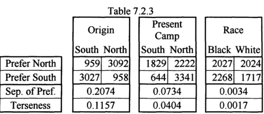
on each other variable severally. Table 7.2.3 shows the separability of Preference and the terseness for all three two-dimensional cross classifications spanned by Preference and one other variable. The greatest separability of Preference, by a large margin, occurs for the 2 × 2 table linking

Preference

with

Origin,

which is also the tersest one.

Which variable is most dependent on the ensemble of all others, disregarding all mutual dependences between the latter?

This differs from Question 3 in that it relates to the dependence of each separate variable on all others, rather than on only one. To answer it, one must succes- sively uncouple all possible combinations of three variables in order to generate all two-entry tables which connect a single variable with the conglomerate of all others. As an example, Table 7.2.4 shows the cross classification obtained through the uncoupling of Preference, Origin, and Present Camp. According to the addition theorem, the static content of this cross classification (0.0653), plus that of the cross classification obtained when removing Race by summation (0.1967), equals the static content of the full original data (0.2620); this can be easily checked (see Table 7.2.2).

Table 7.2.5 lists each variable's separability, given the ensemble of all others, as calculated for Table 7.2.4 and three analogous ones, in each of which a different set of three variables has been uncoupled. Note that Race is least

T a b l e 7.2.4

P r e f / O r i g / C a m p N N N N N S N S N N S S S N N S N S S S N S S S

B l a c k R a c e 876 387 381 383 2 5 0 36 1712 2 7 0 W h i t e R a c e 874 9 5 5 91 104 5 1 0 162 869 176

(21)

Table 7.2.5

Variable

Origin

Preference

Present Camp ...

Race

Separability

0.2912

0.2793

0.1028

0.0945

dependent on all others, although it is Present Camp that contributes least to the overall static content, as was seen in Table 7.2.2.

The above results can be summarized as follows:

1. The least informative variable is Present Camp, closely followed by Race. 2. The tersest representation of knowledge obtainable from the original data is the

2 x 2 table that connects Preference with Origin and neglects the two other variables. 3. Preference depends by far most strongly on the single variable Origin.

4. Origin is the variable most etficiently inferred from all others, closely followed by Preference. Race comes last in this respect.

The analysis provides a compact quantitative view of Stouffer's data by using parameters which allow meaningful comparisons between cross classifications of varying dimen- sionality. It strongly supports one conclusion: "Soldiers want to live near home", and a weak corollary: "The location of his present camp is a much more important consideration for a soldier's preference between North and South than his race" (see Table 7.2.3). 7.3 Finley's Tornado Prediction

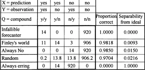
A vexing problem, which to the best of the authors' knowledge has not been solved satisfactorily, was presented by Goodman and Kruskal (1959, p. 127-128): Finley, sergeant in the US Signal Corps, compared his predictions about tornados' occurrence with the actual occurrence. One of Finley's summary tables is given here as an example (Table 7.3.0). As he predicted correctly in 917 (11 + 906) of 934 cases, he gave himself a percentage score of 98.18%. Goodman and Kruskal point out that a completely ignorant person could always predict "No Tornado" and attain a score of 98.50% (920/934), and they conclude "of course, Finley did appreciably better than this 'prediction', the question is that of measuring his skill by a single number."

Consider two separate worlds, that of Finley and an ideal one which is the abode of an infallible forecaster. A sound measure of Finley's skill is the separability between both worlds, the ease with which one can distinguish them when told only that a certain event (a pair prediction/occurrence among the four possible ones: yes/yes, no/yes, yes/no, no/no)