Probabilistic approaches in the effect assessment of toxic chemicals : What are the benefits and limitations?

(1)

Commentaries

Probabilistic Approaches in the Effect Assessment of Toxic Chemicals

What are the Benefits and Limitations?

M a r t i n Scheringer 1, D i r k Steinbach 1, Beate Escher 2 and K o n r a d H u n g e r b i i h l e r 1

1 Laboratory of Chemical Engineering, Swiss Federal Institute of Technology Zfirich, CH-8093 Zfirich, Switzerland 2 Swiss Federal Institute for Environmental Science and Technology (EAWAG) and Department of Environmental Sciences,

Swiss Federal Institute of Technology Zfirich, CH-8600 Dfibendorf, Switzerland

Corresponding author: Martin Scheringer; e-mail: scheringer@tech.chem.ethz.ch

DOh httD://dx.doi.orQ/10.1065/esDr2001.09.091

Abstract. There is an ongoing discussion whether in the environmental risk assessment for chemicals the so called 'deterministic' approach using point estimates of exposure and effect concentrations is still appropriate. Instead, the more detailed and scientifically sounder probabilistic methods that have been developed over the last years are widely recommended. Here, we present the results of a probabilistic effect assessment for the aquatic environment performed for the pesticide methyl parathion and compare them with the results obtained with the com- mon deterministic approach as described in the EU Technical Guidance Document. Methyl parathion was chosen because a sufficient data set (acute toxicity data for about 70 species) was available. The assumptions underlying the probabilistic effect assessment are discussed in the light of the results obtained for methyl parathion. Two important assumptions made by many studies are- (i) a sufficient number of ecologically relevant toxicity data is available, (ii) the toxicity data follow a certain distribution such as log-normal. Considering the scarcity of data for many industrial chemicals, we conclude that these assumptions would not be fulfilled in many cases if the probabilistic assessment was applied to the majority of industrial chemicals. Therefore, despite the well-known limitations of the deterministic approach, it should not be replaced by probabilistic methods unless the assumptions of these methods are carefully checked in each individual case, which would significantly increase the effort for the assessment procedure.

Keywords: Aquatic toxicity; deterministic risk assessment; effect assessment; logit; methyl parathion; probabilistic risk assessment; probit

Introduction

The environmental risk assessment for chemicals requires that dose-effect relationships or at least single toxicity values such as LCs0 describing the occurrence of adverse effects in organisms as a result of certain exposure levels are known. Several existing methods are based on single point estimates of the effect concentrations, often Predicted N o Effect Concentrations (PNECs), which are derived with extrapolation factors from experimental toxicity data and then c o m p a r e d with calculated or measured exposure levels. Ac- cording to the Technical Guidance D o c u m e n t (TGD) of the

EU (EU 1996), the PNEC is obtained for a class of species by selecting the lowest toxicity value from that class of species and dividing it by an extrapolation factor of 10 to 1000, depending on the number and quality of available toxicity data. The option of a statistical evaluation is mentioned only briefly on p. 332 of the T G D and in Appendix V, p. 469. The deterministic approach has been criticised for several reasons (see also section 2.1): the extrapolation factors are arbitrary, the approach utilizes available toxicity data in- completely, and the results are possibly overprotective. In response to such criticism, statistical and probabilistic approaches have been proposed for several years (Kooijman 1987, Wagner and Lokke 1991, Aldenberg and Slob 1993, Suter 1993, Solomon 1996, Solomon et al. 1996, Suter 1998, Klepper et al. 1998). These methods do not compare single exposure and toxicity values, but calculate and compare distributions of exposure and effect values. O n the one hand, these methods utilize the information given in larger data sets m o r e completely and effectively, provided such data sets are available. O n the other hand, they increase data requirements as c o m p a r e d to methods using single data points, which can be seen as a d r a w b a c k if the general lack of toxicity data of industrial chemicals is considered (EEA 1998). Moreover, they are based on several assumptions that are not fulfilled in every case and that have to be checked in the course of the risk assessment (see sections 2.2 and 4). In this study, we conduct a probabilistic effect assessment for methyl parathion with a set of a b o u t 100 toxicity data for aquatic species (Steinbach 1999). On this basis, we in- vestigate the following questions: Is the assumption that toxicity data follow a log-normal or log-logistic distribution fulfilled? W h a t can be done if this assumption is not appli- cable to a given data set? W h a t are the data requirements (total n u m b e r of data, n u m b e r of species, representative- ness of species) of the probabilistic assessment and is it likely that these requirements are met for industrial chemicals? H o w does the result of the probabilistic a p p r o a c h compare with the point estimate of a PNEC according to the T G D ?

1 Data Selection

T h e data selection for this study was influenced by the problem that it is difficult to find broad sets of toxicity data for industrial chemicals. The EU T G D requires a probabilistic

ESPR - Environ Sci & Pollut Res 9 (5) 307 - 314 (2002)

307

(2)

Effect Assessment of Toxic Chemicals

Commentaries

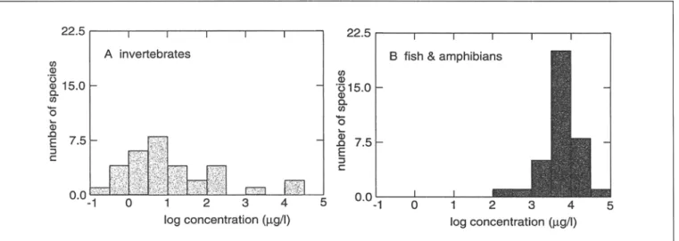
Fig. 1 : Histograms of the 68 LCso values with invertebrates (32 data, left) and vertebrates (fish and amphibia, 36 data, right) shown separately. The total

number of measurements is 104; multiple values for the same species are represented by their geometric mean

assessment to be based on a "large data set from long-term tests for different taxonomic groups" (EU

1996,

p. 469), which is even less likely to be available than LCs0 values. Therefore, methyl parathion (CAS N o . 298-00-0) as a well- investigated pesticide with a specific mode of toxic action (inhibition of acetyl choline esterase) for which a relatively large data set is available (Hertel 1993) was chosen here as an exemplary chemical. However, these data are acute LCs0 values and not N o Observed Effect Concentrations (NOECs) from long-term tests. H o w a PNEC value might be derived from the results of the statistical analysis of the LCs0 data remains to be discussed.

The registration of pesticides requires a much more exten- sive testing procedure than the illustrative calculation of hazardous concentrations shown here. The purpose of the methyl parathion example is not to discuss the testing procedure for pesticides, but is to illustrate the application of the probabilistic assessment that is currently discussed for industrial chemicals too.

LCs0 values for aquatic species (insects, fish, estuarine species such as mussels, shrimps, crabs, water fleas, etc.) were taken from Hertel et al. (1993) and 3 ECs0 values for algae were obtained from the database P R E D O C of the Swiss Agency of the Environment, Forests and Landscape. Most of the underlying tests were static; the test duration was 24, 48, or 96 hours. In cases where results for different test du- rations are given for the same species, the toxicity values with the longest duration were used. When multiple values were available for the same species and identical conditions, the geometric mean was used. This selection leads to a set of 71 LCs0 and ECs0 data which is depicted in Fig. 1 (without the three 3 algae).

The histogram shows mainly two clusters which correspond to the different toxicity of methyl parathion to invertebrates such as crustaceae, insects, and to molluscs and vertebrates (here: fish and amphibia). The difference in toxicity between the two groups is caused by differences in activation and detoxification processes and differences in modes of toxic action (Legierse 1998).

2 M e t h o d s

2.1 Point e s t i m a t e s for P r e d i c t e d N o Effect C o n c e n t r a t i o n s

The deterministic approach according to the EU T G D (EU 1996) aims at calculating a Predicted N o Effect Concentra- tion (PNEC) from experimental toxicity data. Depending on the amount and type of data (acute LCs0 vs. long-term NOECs), different extrapolation factors are used for calculating the PNEC (EU 1996, p. 330). If there are several toxicity data for a class of species, the lowest values are used for this extrapolation.

Problems associated with this procedure are.

1. The PNEC value can be seen as overprotective since it is derived from the lowest toxicity value that is available. N e w data lead to still lower PNEC values if they are lower than previous measurements; otherwise, they do not influence the existing PNEC value.

2. On the other hand, the P N E C value can be seen as underprotective since it does n o t reflect effects occurring on a population or ecosystem level as pointed out by Hammers-Wirtz and Ratte (2000). The species showing the lowest toxicity score in laboratory tests is not a 'sen- tinel' species of relevant ecosystems (Power and McCar- thy 1997), i.e. protection of this species does not guar- antee ecosystem protection.

3. The scientific basis of the extrapolation factors is often weak (Chapman et al. 1998, Koller et al 2000, Duke and Taggart 2000).

2.2 Statistical evaluation

The statistical and probabilistic assessment methods rest on the idea that the species chosen for obtaining experimental toxicity data represent a random selection from a larger community of species so that the distribution of the toxicity data of all these species can be estimated with statistical methods from the set of experimental toxicity data. In many cases a certain distribution, e.g. log-normal or log-logistic, of the over- all toxicity data is assumed (Kooijman 1987, Aldenberg and Slob 1993) and estimates of the mean and standard deviation

(3)

of this distribution are calculated from the experimental data. In the statistical evaluation, the distribution is then linearized by the corresponding logit or probit transformation (Solomon et al. 1996, Solomon et al. 2001) and hazardous concentrations are determined, which are defined as the concentrations at which the toxicity thresholds (LCs0 or NOEC) are exceeded for a certain fraction of species. The main contribution of this approach is that it accounts for the inter-species variability of the susceptibility to a chemical.

Although the procedure seems straightforward, there are several difficulties associated with it (Newman et al. 2000). Here, we first demonstrate the procedure and calculate some results for the example of methyl parathion; subsequently, we discuss its difficulties and limitations.

In the first step, the logarithms of the

LCso

values are ranked (log LCs0 is denoted by x in the following); for each value x, the rank rx is obtained as r~ =

j/(N +

1) where N is the total number of toxicity data, here 71, and j runs from 1 to N. (The value N + 1 is used in order to avoid the result r~ = 1 for j -- N because the theoretical cumulative distribution does not reach r~ = 1 at finite numbers of data, N, and finite concentrations, x.) The rank r x is the fraction of the N toxicity values that are lower than or equal to x. If r~ is plotted against the toxicity values (concentrations on a logarithmic scale), this leads from a histogram such as in Fig. 1 to a cumulative frequency distribution. In the cases of the ideal

normal or logistic distributions, this cumulative frequency distribution is given by the functions

~(x)

and

A(x)

with

1

"

[ 1(_~)]

cumulative normal

~(x) - 4"~ucr Sexp - dr" distribution (la)

A(x) = (1 + exp[.Zc(~.~3x) ])-' cumulative logistic _distribution _(lb)

la and ~ are the mean and standard deviation; two examples for

A(x)

with different g and o are shown in Fig. 2 (top right). Then the y axis of this plot of the cumulative frequency distribution is transformed such that it indicates units of ~ from the theoretical distribution, here normal or logistic, in equal distances (probit or logit units). In order to obtain positive values for most data points except for those below la - 5 c, the mean value is assigned to a probit value of y = 5 by convention. This transformation means that the upper and lower end of the y axis are stretched while the middle part is compressed in such a way that a normal or logistic distribution appears as a linear function (shown for logistic distribution in Fig. 2, bottom). The transformation is carried out by applying the inverse of the cumulative distribution functions, here denoted by PT and LT, to the r x values indicated on the y axis: 0.12 O.lO 0 0.08 .CI E ~= 0.06 "5 ~- 0.04 .o ~ 0 . 0 2 / % 1 ' / t , I I.t=25 I % , i ~ = 2 0 . 8 logistic , d i s t r i b u t i o n s , I t I | , l ~-~ 0 . 6 I t , l -~

//\,,

o , I~ = 20

\

0.2 1 0 2 0 30 40 log c o n c e n t r a t i o n cumulative logistic distributions, , i ' 7 d e n o t e d by A(x) in eq. l b / / /

jjjj/I

10 20 30 40 log c o n c e n t r a t i o n cumulative logistic ,.." distributions a f t e r ,,"" " ~ 1 0 = I o g i t - t r a n s f o r m ~ . 1 r _o 5 ss SSS . . . . . . 9 | . . . . I

10 I o

2~

40

9 ~5Yo

log C;ha z log Ch5~ log c o n c e n t r a t i o n

Fig. 2- Linearization of the logistic distribution. Top: two different logistic distributions (left) and their cumulative representations (right), bottom: Iogit plot of the two cumulative distributions

(4)

Effect Assessment of Toxic Chemicals

Commentaries

eT(r) = O-~(r)

with p = 5 and o = 1 in

~-~(x)

(2a)

(probit tranformation)

Lr(r ) = A-'(r) = # + G'[~ in [ r---~-- ] z c " [ l - r ]

with I J = 5 and o = 1 (2b)

(logit transformation)

After this transformation, probit or logit units are given on the y axis (the x axis shows the logarithms of the toxicity data). Linear relationships PT vS. X and L v vs. x result if the data are distributed log-normally or log-logistically. From the experimental data points, a regression line showing the deviation of the data from the ideal distribution is calculated. This procedure gives a quantitative understanding of the interspecies variability (which is completely neglected in the single-point approach).

Next, the hazardous concentration is derived, which is defined as the concentration exceeding the toxicity threshold (here: acute toxicity) for a certain fraction of the total number of species, often 5% or 10%. These percentages correspond to probit values of 3.355 and 3.718 and to logit values of

3.377

and

3.789,

i.e. the hazardous concentration is given by the point on the x axis at which the regression line reaches the above probit or logit values (Fig. 2, bottom). Finally, the linearized distribution of toxicity data can be compared with a distribution of exposure data and the over- lap between the two distributions indicates which fraction of species is exposed to which concentration level (exceedence plot, not presented here).

C s~ with a certain probability, e.g. 50% or haz

95%. L

is determined according to

L = ~N - k~' .s~ (3)

where 2 N and s~ are the mean and standard deviation of the logarithmic toxicity values of the sample of N species. k~ is an extrapolation constant depending on N and the selected confidence limit. Aldenberg and Slob (1993) provide k~ values for various N from 2 to 500 and for confidence limits of 95% and 50%. The k~ values are determined such that the confidence limits are below the true value of C ~ with probabilities of 95% and 50% (Aldenberg and Slob 1993).

3 Results

3.1 Calculation of the PNEC with extrapolation factors

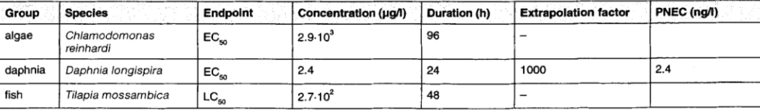
The lowest ECs0 and LCs0 data for the three classes of algae, daphnia, and fish are shown in Table 1. Since all these data are from acute tests, an extrapolation factor of 1000 is applied to the lowest value (2.4 pg/1 for

Daphnia longispira),

leading to a PNEC of 2.4 ng/1. This value is rather low due to the high susceptibility of daphnia to methyl parathion. If additional species such as mysid shrimp

(Mysidopsis bahia)

with lower LCs0 values than daphnia are included, PNECs even below 1.0 ng/1 are obtained. According to the TGD, such 'non-standard' organisms might be considered in the assessment, in which case they have to be assigned to the appropriate trophic levels (EU 1996, p. 323).

2.3 Probabilistic evaluation

The methods of Aldenberg and Slob (1993), following Kooij- man (1987) and van Straalen and Denneman (1989), and of Wagner and Lokke ( 1991 ), make it possible to calculate confidence limits of the hazardous concentration C ~ , depending on the sample size. This means that not only a single estimate of C ~ is determined (as it is provided by the statistical analysis), but that the probability that the estimated value exceeds the true value of C ~ is included too. The basic assumption of these methods is that the species sensi- tivities follow log-normal (Wagner and L~kke) or log-logistic distributions (Kooijman 1987, van Straalen and Denne- man 1989, Aldenberg and Slob 1993). Here, we only briefly describe the calculation procedure; for the mathematical background, see the original papers.

The confidence limit L (here in pg/l) is the concentration that is below the true value of the hazardous concentration

3.2 Statistical evaluation

If the procedure described in section 2.2 is applied to the 71 LCs0 and ECs0 values selected for methyl parathion, the plots shown in Figs. 3 and 4 are obtained.

The two clusters visible in Fig. 1 correspond to the systematic deviations of the data points from the regression lines. Nei- ther the logistic nor the normal distribution fits the data; without any statistical test it is obvious that both are not adequate and that the choice between these two linearization methods is not significant for the quality of the results. The hazardous concentrations C ~ are 0.45 pg/1 (probit) and 0.35 pg/1 (logit); C 1~ is obtained similarly (not shown in the figures); see val- haz

ues given in Table 2. The C ~ values are somewhat lower than the C ~ of 3.4 pg/l obtained by Newman et al. (2000) for a set of 42 methyl parathion LCs0 data.

Table 1: Selected acute toxicity data and PNEC values of methyl parathion according to the EU TGD. The data are for adult organisms of the most

susceptible species among the three groups of algae (total: 3 data), daphnia (total: 4 data), and fish (total: 58 data)

Group ' Species

algae Chlamodomonas

reinhardi

daphnia Daphnia Iongispira

fish Tilapia mossambica

Endpolnt

ECso

ECso LCso

'Concentration (pg/I) i Duration (h) '

2.9.10 a 96

2.4 24

2.7.102 48

Extrapolation factor PNEC (ng/I)

1000 2.4

(5)

8 A -~ y = 0 . 5 7 x + 3 . 5 5 3.36 ~- zx I 2 I 1 I I 0 . . . . ' - 9 q - : . . . . '. . . . . : . . . . : . . . . : . . . . 9 . . . . i -2 -1 I 0 1 2 3 4 6 6 5% log Cha z l o g c o n c e n t r a t i o n ( l x g / I ) Fig. 3: Regression analysis of the complete data set after probit transformation. The hazardous concentration C 5% h.z is 0.45 pg/I

8 7 "E ~ 6 c~ 5 o 4 3.38-- 3 2 1 0 A y = 0 . 5 5 X + 3.61 ~ZX A .. .. [ .. .. = ' ' ' ' I ' . . . ' ' ' I ... . ; . ... ', .. .. -2 -1 0 1 2 3 4 5 6 ) 5~ l o g c o n c e n t r a t i o n (Ixg/I) log Cha z

Fig. 4: Regression analysis of the complete data set after Iogit transformation. The hazardous concentration C 5% h~ is 0.35 pg/I

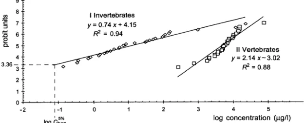
Because the assumption that the complete data set repre- sents a normal or logistic distribution is not fulfilled, the two clusters s h o w n in Fig. i are analyzed separately in the following. The h a z a r d o u s concentration c a n then be determined for each of the clusters, which leads to 0.084 ilg/1 (probit) and 0.068 lag/l (Iogit) for the more susceptible species (invertebrates) and to 9.5-102 pg/1 (probit) and 9.1.102 pg/l (logit) for the vertebrates (Figs. 5 and 6, Table 2).

The regression p a r a m e t e r s R 2 are s o m e w h a t higher for the separate clusters than for the complete data set. Although there are still systematic deviations, it is discernible that groups of t a x o n o m i c a l l y m o r e similar species show a more regular distribution than a very heterogeneous set (Wagner and L~kke 1991).

The choice of the set of relevant species strongly influences the results for C ~ . The results for the invertebrates are lower than the values obtained f r o m the complete data set by a factor of a b o u t 5 while C ~ for the vertebrates is higher by a factor of 2.103. N o t e that no extrapolation factors have been applied and t h a t these results are still to be interpreted in terms of acute LCs0 data. If a generic acute-to-chronic

ratio of 1 5 - 2 5 is assumed (L/inge et al. 1998), such a value might be used as an extrapolation factor to derive a chronic hazardous concentration f r o m the C 5~ values. haz

3 , 3 P r o b a b i l i s t i c e v a l u a t i o n

As the method of Aldenberg and Slob requires logistically distributed data and because this requirement is fulfilled to a higher extent by the individual clusters, we a p p l y this method to the t w o clusters separately. The means a n d standard deviations o f the t w o data sets are given in Table 3. Extrapolation constants interpolated from the values given by Aldenberg and Slob (1993, p 55) are kff = 2.19 (95% confidence) and 1.65 (50% confidence) for the vertebrates with N = 36 and k~ r = 2.22 (95% confidence) and 1.65 (50% confidence) for the invertebrates with N = 32. If applied according to eq. 3, these kff values yield the confidence limits

Lss

and

Lso. The

numerical values of

Lgs

and

Lso

(see Table 3) include the C ~ values from the regression analysis, which indicates some consistency of the methods.

(6)

Effect A s s e s s m e n t of T o x i c C h e m i c a l s C o m m e n t a r i e s ~ ~- - 7 I I n v e r t e b r a t e s ~ , , , , , , , , , , , ~ o ~ , / r ~ -~ y = 0 . 7 4 x + 4 . 1 5

z f

4 ~ " ~.7"~ L-F y = 2.14 x-3.02 3.36 -~ -- -- -- o r l J R 2 = 0 . 8 8 f 2 1 0 . . . . 1 ' " " " ; . . . . ', . . . . : . . . . ~ . . . . ~ . . . . : " " " - 2 -1 0 1 2 3 4 5

5~176 log concentration (~g/I)

log Cha z

Fig. 5: Separate regression analyses of the data sets for invertebrates (I) and vertebrates (11), after probit transformation. The hazardous concentration derived from the cluster I is C ~ = 0.084 pg/I

9 .-_= 8 r - 7 o 6 5 4 3 . 3 8 - - 3- 2 1 0 -2 I Invertebrates ~ < > J o y = 0.71 x + 4 . 1 8 . ~ ~ R 2 = 0.94 ^ < ~ > ~ ~ " = ) " ~ ~ _ _ _ . ~ II V e r t e b r a t e s = y = 2.08 x-2.81 - - - - - I o [ 3 J R 2 = 0 . 9 1 I I I , , , , I I . . . . : . . . . , . . . . : . . . . : . . . . : . . . . : . . . . ,, i-1 0 1 2 3 4 5 6

15~ log concentration (p.g/I)

log Cha z

Fig. 6: Separate regression analyses of the data sets for invertebrates (I) and vertebrates (V), after Iogit transformation. The hazardous concentration derived from the cluster I is C ~ = 0.068 pg/I

T a b l e 2: Hazardous concentrations C s~ ha~ and C ~~ ~ derived by statistical analysis for methyl parathion

' . . . . R e g r e s s i o n D i s ~ i b o t i o n D a t a s e t . . . . normal a all data P a r a m e t e r s b 0.57 3.55 invertebrates 0.74 4.15 vertebrates 2.14 - 3 . 0 2

logistic all data 0.55 3.61

4.18 invertebrates 0.71 vertebrates 2.08 -2.81 4.5.10 -~ 8.4.10 -2 9.5.102 3.5.10 -1

c,O

_ . h a z I J g / I 2.0 2.6.10 -1 1.4.103 1.6 6.8.10 -2 9.1.102 1.4.103 2.2.10 -1

T a b l e 3: M e a n values and standard deviations of the two data subsets as well as confidence limits Z ~ and /-~0~ of Ch~ (in pg/I) derived for methyl parathion with extrapolation constants from Aldenberg and Slob (1993). ~ and s m are logarithmic values

inverteb rates 1.14 1.21 2.8-104 1.4-10 -1

vertebrates 3.75 0.41 7.1.102 1.2-103

(7)

4 Discussion and C o n c l u s i o n s

The statistical analysis of the toxicity data for methyl parathion shows that the available data do not follow a certain distribution such as log-normal or log-logistic. In contrast, the distribution is bimodal with two clusters of more and less susceptible species, the latter containing mainly fish. Accordingly, the choice of the probit or logit transformation does not influence the results of the analysis significantly. However, the results depend strongly on the choice of a certain (sub) set of data and the fraction of species defin- ing the hazardous concentration (5% or 10%). In the methyl parathion example, it was fairly easy to distinguish two clusters and to rationalize the distinction biologically, which, however, might not be the case for other compounds. Further, the lack of chronic data even for a well-investigated pesticide such as methyl parathion illustrates that the requirements stated in the EU TGD - that the statistical analysis should be based on a large set of long-term NOEC data - is very unlikely to be fulfilled for industrial chemicals. If, as in our case, acute data are used instead, the hazardous concentrations derived for methyl parathion are much higher than the PNEC obtained by extrapolation from a low acute LCs0. If this hazardous concentration was used directly as a level for tolerable effects, significant impacts might be possible. On the other hand, if a PNEC is to be derived from the hazardous concentration, this question cannot be solved in a more satis- factorily manner than in the deterministic approach.

Several of our findings are in line with the conclusions drawn by Emans et al. (1991) in a study comparing different probabilistic methods and several chemicals. They give rise to some further considerations:

1. The assumption that the species whose toxicity data are available (and to which many studies will be restricted for practical reasons) represent a random selection from a complete 'universe of species' is not fulfilled. The boot- strap approach proposed by Newman et al. (2000) and the method of van der Hoeven (2001) offer opportuni- ties to avoid the problem of selecting a certain theoretical distribution.

2. The 'universe of species' has to be specified in terms of species that are representative for a certain ecosystem. This is an essential requirement underlying the statistical approach, which is also stated by Wagner and Lokke (1991) and further discussed by Forbes and Forbes (1993). An example meeting this requirement is provided by the US Water Quality Guidance for the Great Lakes System where eight families are specified that have to be represented by at least one species each (CFR 1995). Wagner and L~kke (1991) point further out that the chosen species should be rather close in terms of 'taxonomic distance' and that the data should represent the same endpoints.

3. The number of species included into the analysis has to be high enough. N e w m a n et al. (2000) give a number of about 30 data points required to minimize the uncertainty of their C ~ estimates. The extrapolation method of Aldenberg and Slob can in theory be applied to small

data sets, but, in practice, the assumption that the data are distributed logistically has to be checked and this requires at least 10 data points. The same requirement has to be met for probit or logit transformation and sub- sequent regression analysis.

4. Provided the foregoing requirements are fulfilled, it is a further question if the level of acceptable ecosystem damage (given by a fraction of affected species, e.g. 5%) can be chosen in a reliable way. This would require a politi- cal and societal debate about what fractions of species might be endangered in what kind of ecosystems (for all ecosystems possibly exposed to the chemical). It is unlikely that such a complex decision can be made in a satisfactory way. By accepting ecosystem damage a priori,

the aim of finding a no-effect level concentration level is abandoned and the hazardous concentrations might be underprotective.

5. As pointed out by Suter (1998), the probabilistic methods lend support to a conceptual misunderstanding: When a set of toxicity data for various species is seen as a descrip- tion of the susceptibility of a community such as an ecosystem (which is a necessary interpretation, see item 2 above), the statistical analysis of this set of data provides fractions of species affected by a certain concentration of the chemical under consideration. These fractions are 'deterministic' measures of effect on the community level; the statistical analysis does not provide probabilities of the occurrence of these effects. Such probabilities can only be determined by quantifying the uncertainties (or confidence limits) of the percentiles of the species sensitivity distributions (Suter 1998, 3). This is, e.g., included in the approaches proposed by Kooijman (1987), van Straalen and Denneman (1989), Wagner and L~kke (1991) and Alden- berg and Slob (1993) and is an additional step going be- yond the mere statistical analysis.

6. It is not clear whether and, if yes, h o w the results obtained by statistical or probabilistic extrapolation from a set of acute LCso data can be compared to PNEC values. The probabilistic approach accounts for the interspecies variability of a given set of data but - due to its very different basic assumptions - does not provide a substitute for the deterministic calculation of a PNEC. For chemicals with sufficient and reliable toxicity data (see above, items 1 to 3), it should be used complemen- tary to the calculation of the PNEC.

In conclusion: There is no doubt that the single-point approach according to the EU TGD is not satisfactory for many reasons. However, it does not seem appropriate to replace this approach by a more elaborate statistical or probabilistic analysis that evaluates the species sensitivity distribution of a specific set of toxicity data, but gives no hint for the extrapolation from acute to chronic, from short term to long term, or from laboratory to field conditions.

I Acknowledgment.

We thank K. Becker van Slooten, H. Ehrhardt, B. l

Minten, and C. Studer

for their

support in this study.

(8)

Effect Assessment of Toxic Chemicals

Commentaries

References

Aldenberg T, Slob W (1993): Confidence Limits for Hazardous Concentrations Based on Logistically Distributed NOEC Data. Ecotox Environ Safety 25, 4-63

Chapman PM, Caldwell RS, Chapman PF (1996): A Warning: NOECs are Inappropriate for Regulatory Use. Environ Toxicol Chem 15, 77-79

Chapman PM, Fairbrother A, Brown D (1998): A Critical Evalua- tion of Safety (Uncertainty) Factors for Ecological Risk Assess- ment. Environ Toxicol Chem 17, 99-108

CFR (1995): Code of Federal Regulations, Title 40, Part 132: Wa- ter Quality Guidance for the Great Lakes System. United States Government Printing Office

Duke DL, Taggart M (2000): Uncertainty Factors in Screening Eco- logical Risk Assessments. Environ Toxicol Chem 19, 1668-1680 EEA (1998): Chemicals in the European Environment: Low Doses,

High Stakes? European Environment Agency, Copenhagen Emans HJB, v. d. Plassche EJ, Canton JH, Okkerman PC, Sparen-

burg PM (1993): Validation of some Extrapolation Methods Used for Effect Assessment. Environ Toxicol Chem 12, 2139-2154 EU (1996): Technical Guidance Document in Support of Commis-

sion Directive 93/67/EEC on Risk Assessment for New Notified

Substances and Commission Regulation (EC) 1488/94 on Risk Assessment for Existing Substances. Office for Official Publica- tions of the European Communities

Forbes TL, Forbes VE (1993): A Critique of the Use of Distribu- tion-Based Extrapolation Models in Ecotoxicology. Functional Ecology 7, 249-254

Hammers-Wirtz M, Ratte HT (2000): Offspring Fitness in Daph- nia: Is the Daphnia Reproduction Test Appropriate for Extrapo- lating Effects on the Population Level? Environ Toxicol Chem 19, 1856-1866

Hertel R (1993): Environmental Health Criteria 145: Methyl parathion. World Health Organization

Klepper O, Bakker J, Traast TP, Van de Meent D (1998): Mapping the Potentially Affected Fraction of Species (PAF) as a Basis for Comparison Ecotoxicological Risks between Substances and Re- gions. J Hazard Mat 61,337-344

Kooijman SALM (1987): A Safety Factor for LCs0 Values Allow- ing for Differences in Sensitivity among Species. Wat Res 21, 269-276

Koller G, Hungerbiihler K, Fent K (2000): Data Ranges in Aquatic Toxicity of Chemicals. ESPR - Environ Sci & Pollut Res 7, 135-143

L~inge R, Hutchinson TH, Scholz N, Solb6 J (1998): Analysis of the ECETOC Aquatic Toxicity (EAT) Database II: Comparison of Acute to Chronic Ratios for Various Aquatic Organisms and Chemical Substances. Chemosphere 36, 115-127

Legierse K C H M (1998): Differences in Sensitivity of Aquatic Organisms to Organophosphorus pesticides, Ph.D. Dissertation, University of Utrecht, The Netherlands

Newman MC, Ownby DR, M6zin LCA, Powell DC, Christensen TRL, Lerberg SB, Anderson B-A (2000): Applying Species-Sen- sitivity Distributions in Ecological Risk Assessment: Assump- tions of Distribution Type and Sufficient Numbers of Species.

Environ Toxicol Chem 19, 508-515

Power M, McCarthy LS (1997): Fallacies in Ecological Risk As- sessment Practices. Environ Sci Technol 31, 370A-375A Solomon KR et al. (1996): Ecological Risk Assessment of Atrazine

in North American Surface Waters. Environ Toxicol Chem 15, 31-76

Solomon KR (1996): Overview of Recent Developments in Ecotoxicological Risk Assessment. Risk Anal 15,627-633 Solomon KR, Giddings JM, Maund SJ (2001): Probabilistic Risk

Assessment of Cotton Pyrethroids: I. Distributional Analysis of Laboratory Aquatic Toxicity Data. Environ Toxicol Chem 20, 652-659

Steinbach D (1999): Diploma thesis. ETH Ziirich

Suter GW (1993): Ecological Risk Assessment. Lewis Publishers, Chelsea, MI, USA

Surer GW (1998): Comments on the Interpretation of Distribu- tions in 'Overview of Recent Developments in Ecological Risk Assessment'. Risk Anal 18, 3-4

Van der Hoeven N (2001): Estimating the 5-Percentile of the Spe- cies Sensitivity Distributions without any Assumptions about the Distribution. Ecotoxicology 10, 25-34

Van Straalen NM, Denneman CAJ (1989): Ecotoxicological Evalua- tion of Soil Quality Criteria. Ecotox Environ Safety 18, 241-251 Wagner C, L~kke H (1991): Estimation of Ecotoxicological Protec- tion Levels from NOEC Toxicity Data. Wat Res 25, 1237-1242

Received: March 21st, 2001 Accepted: September 16th, 2001

OnlineFirst- September 30th, 2001

L.. Martin Scheringer holds a diploma in chemistry and a PhD in environmental sciences. Presently, he is a research associate with the B Safety and Environmental Technology Group at the Department of Chemistry of the Swiss Federal Institute of Technology ZLirich. In his R research he investigates methods for the assessment of the environmental fate and effects of chemical products with particular focus on m the two indicators of persistence and spatial range (see ESPR 8, 2001, No. 3, pp. 150-155). The present study is based on the results of the diploma thesis of D. Steinbach, which was supervised by M. Scheringer and B. Escher and supported by a working group with members from different research institutes, authorities and industry: Dr. Kristin Becker van Slooten, Swiss Federal Institute of Technology Lausanne; Dr. Horst Ehrhardt, Solvias AG; Dr. Barbara Minten, Registration and Consulting Company Ltd (RCC); Dr. Christoph Studer,

Swiss Agency for the Environment, Forests and Landscape. ~ ~ J