Discrete event front tracking simulator of a physical fire spread model

HAL Id: hal-00438619

https://hal.archives-ouvertes.fr/hal-00438619

HAL is a multi-disciplinary open access archive for the deposit and dissemination of sci-entific research documents, whether they are pub-lished or not. The documents may come from teaching and research institutions in France or abroad, or from public or private research centers.

L’archive ouverte pluridisciplinaire HAL, est destinée au dépôt et à la diffusion de documents scientifiques de niveau recherche, publiés ou non, émanant des établissements d’enseignement et de recherche français ou étrangers, des laboratoires publics ou privés.

Discrete event front tracking simulator of a physical fire

spread model

Jean Baptiste Filippi, F. Morandini, Jacques-Henri Balbi, David R.C. Hill

To cite this version:

Jean Baptiste Filippi, F. Morandini, Jacques-Henri Balbi, David R.C. Hill. Discrete event front tracking simulator of a physical fire spread model. SIMULATION, SAGE Publications, 2009, 86 (10), pp.629-644. �10.1177/0037549709343117�. �hal-00438619�

Discrete event front tracking simulator of a physical

fire spread model

J.B. Filippi*

_{, F.Morandini}

_{, J.H. Balbi}

_{, D. Hill²}

UMR CNRS 6134

Systèmes physiques pour l'environnement University of Corsica

Corte, France

²ISIMA/LIMOS UMR CNRS 6158

Computer Science & Modeling Laboratory Blaise Pascal University

Keywords:

Fire spread, DEVS, simulation, asynchronous, discrete events, flame, forest, envelope, interface, front tracking

* Corresponding author

Email address: filippi@univ-corse.fr (J.B. Filippi).

hal-00438619, version 1 - 4 Dec 2009

Author manuscript, published in "Simulation (2009) accepted, online, identifiant pending" DOI : 10.1177/0037549709343117

Abstract

Simulation of moving interfaces, like a fire front usually requires the resolution of a large scale and detailed domain. Such computing involves the use of supercomputers to process the large amount of data and calculations. This limitation is mainly due to the fact that large scale of space and time is usually split into nodes, cells or matrices, and the solving methods often require small time steps. This paper presents a novel method that enables the simulation of large scale/high resolution systems by focusing on the interface. Unlike the conventional explicit and implicit integration schemes, it is based on the discrete-event approach, which describes time advance in terms of increments of physical quantities rather than discrete time stepping. Space as well is not split into discrete nodes or cells, but we use polygons with real coordinates. The system is described by the behaviour of its interface, and evolves by computing collision events of this interface in the simulation. As this simulation technique is suited for a class of models that can explicitly provide rate of spread for a given configuration, we developed a specific radiation based propagation model of physical wildland fire. Simulations of a real large scale fire performed with an implementation of our method provide very interesting results in less than 30 seconds with a 3 metres resolution with current personal computers.

1 Introduction

Simulation of a spatial phenomenon requires the description of an environment in a way that can be efficiently processed by a computer, and adapted to numerical manipulations. Typically, in forest fire the phenomenon is evolving on an area composed of non burnable roads, rivers and fuel breaks and burnable large patches of uniform land. One of the main problems of this spatial distribution is that non burnable areas have strong effects on propagation dynamics despite being several orders of magnitude smaller than the burnable areas.

In order to take into account all details, most simulation techniques discretize space and time in more or less regular meshes, or grids, and use those mesh to solve the model. Using a mesh implies that before performing a simulation, a trade-off must be made between resolution and size of the domain, as a computer will only be able to process a limited amount of nodes or cells. A large forest fire will spread over an area greater than 100 Km², at best a 2 meter of resolution is needed to take into account roads and fuel breaks, and thus 25 million cells are necessary which greatly impact simulation time and memory usage.

There are many ways to work around those limitations, increasing computer speed and memory, distributing calculus when it is possible, or optimizing the algorithms is a good way to enhance performance.

Nevertheless, such large fire will develop in a few hours, and require a forecast that can be delivered in a few minutes in order to try different fire fighting scenarios.

The goal of the work proposed in this paper is to propose a method that is able to simulate in a few minutes the propagation of a large wild fire at a high resolution.

For that we propose to work around the limitations of current methods by using a different representation of the environment and the phenomenon.

The proposed method combines discrete event simulation Zeigler (2000) and front tracking (Glimm et al. 1996), (Du et al. 2006), (Risebro and Holden 2002), (Risebro and Tveito 1992). Front tracking methods are used to study physical interface or boundary dynamics. The physical interface is defined here as the frontier line between two state of a system.

For example, a model of a sea oil slick may be defined by with two states: oil is present and oil is absent. In a forest fire model, the two states for the vegetation are burnt and un-burnt, and the fire front is the interface between those two states.

While common methods simulate the spatial evolution of the state of the system, front tracking methods are designed to directly simulate the spatial evolution of the frontier between those two states. With this view on system, the environment can be described in a different fashion because interfaces can be processed as a set of points or vertices with continuous coordinates. The entire map on which the system is evolving does not need to be discrete in order to study interface dynamics. Map state can be a function of the location (a hill can be described by a sine function) as long as it is possible to evaluate a state for a given set of coordinates.

Front tracking has been seldom applied to forest fire simulation, in the proposed approach it is coupled with discrete event simulation (DES) as opposed to discrete time simulation. If discrete time stepping is used, the resolution of the system falls in the similar limitations as with regular meshes; trade-offs have to be made between temporal resolution and temporal scale of the simulation. Describing front models as discrete event systems permits to define time as a continuous value, like the other dimensions of the system and domain, simulation then becomes asynchronous in an approach similar to Karimabadi et al (2005).

The following part presents a review of related work on front tracking, asynchronous simulation and fire spread simulation. The overall simulation method, concepts and detailed simulation algorithms are presented in the third part of the article. The proposed physical fire rate of spread model is described in the fourth section.

The last part of the paper presents simulations and an implementation of the fire model that shows that the method is appropriate to simulate in a few minutes the evolution of large wildfires at high resolution.

2 Background

Topics of interest related to this study are transversal to discrete event simulation, numerical simulation, front tracking methods and fire propagation. The general problem that motivates the development of the method was to find a suitable method to perform quickly a physical simulation of fire spread on a wide domain.

Fire spread models are generally classified in three families (Pastor 2003), empirical, semi-empirical and physical. Empirical models try to capture the behaviour of a front using purely statistical and stochastic methods based on observation. Quasi empirical models, such as the one proposed by Rothermel (1972), are the most widely used and derive from a physical formulation of the problem, but include some parameters that are deduced (fitted) from observations. Physical models attempt to represents the behaviour of a wild fire with no fitted parameters; among those, complex multi-phasic models attempts to represents both combustion and propagation, while reduced physical models are focused only on propagation.

Advantages of physical models are that more diagnoses can be derived from the simulation, such as the fire intensity or emission of atmospheric pollutants. Physical models are also more generic, since empirical and quasi empirical models can only reproduce a fire behaviour that has already been observed (Pastor 2003). The interested reader will find in Sullivan (Sullivan, 2006) a summary of currently available forest fire models.

Simulation results of different models, may not be directly comparable, for example, the rate of spread will be diagnostic (usually deduced from a fully resolved temperature field) in a complex physical model, while it will be prognostic (directly calculated) in a reduced physical, empirical and quasi-empirical models.

Complex models are also usually more calculation intensive, and therefore restrained to either smaller domains or will take more time to calculate than the actual wildfire will take to propagate. Consequently, numerical methods adapted to simulate those models can be very different, from finite elements methods (Linn, 2002) to ellipse reconstruction (Finney and Andrews, 1994), front tracking (Mallet et al, 2007), DEVS-based cellular simulation (Ntaimo et al, 2004), (Vasconcelos and Guertin, 1992), (Muzy et al, 2005) or even with cellular automaton (Dunn and Milne, 2004). Cellular automata methods in the field of forest fire and DES has also been the field of numerous studies that shown interesting results but are often limited to a certain resolution in order to have sufficiently fast simulation time for larger domains. Moreover, the approach developed in this work is very different as cellular models as it does not require a regular mesh or cell. A complete description of the numerous cell based models of fire spread will be out of the scope of this paper. Most work done in the field of numerical methods of fire spread has been done with models that prognoses the Rate of Spread (RoS). RoS for every portion of the front is then used to reconstruct the shape of the fire over time from an initial solution.

Among the reconstruction methods, the most commonly used is the method of ellipses where ellipses the size of a fire advance for a given time step are drawn around an initial front to reconstruct the front one step forward.

We will be more interested here in the family of front tracking methods from which the proposed method is derived.

Front tracking is the general denomination for any numerical scheme that calculates the movement of an interface between two phases of a system (burnt/unburnt, water/oil, etc…). Of those methods, three main approaches are relevant for the simulation of fire fronts.

In volume of fluid method (Hirt and Nichols, 1981), the front is represented by a plane in a grid cell, and the volume of each phase is estimated by the amount of each grid cell in each part of the plane. Such methods usually represent well topological changes of the front and are adequate to perform a budget for any physical variable of each phase; nevertheless, as the front is approximated locally as a straight line parallel to the mesh, it is difficult to evaluate the norm vector of the front advance which is critical in fire spread models.

For problems where performing budgets are less critical, the most common approach is the level set method (Mallet et al, 2007). Like volume of fluid method, a level set method requires the use of a grid to calculate the position of the interface, the main advantage of level set method is that it directly deals with topological problems (such as front merging and convergence). An application of the level set method to forest fire spread model can be found in Mallet et al. (2007). Some computationally efficient algorithms exits for the level set method but implies automatic refinement of the grid near the interface using memory intensive data structure and therefore may limit the size of the simulated domain.

Finally marker method are also used for the resolution of front tracking (Lallemand et al, 2007); in this method, the front is discretized by a set of points, at each step markers are moved according to a speed function. With this low-computational cost Lagrangian technique it is possible to simulate the evolution of an interface without an underlying grid to represents the state of the system. The method proposed in this paper derives from the marker method. As stated earlier, one of the main problems in forest fire modelling is that the phenomenon is evolving on large patches of uniform condition with a few small scale details that have strong effects on the propagation. Using this method helps overcoming this problem as large uniform patches, small roads or even large rocks can be represented as arbitrarily shaped polygons and no underlying matrix to represent the state of the system. The main problem of this method is that collision or intersection must be checked each time a marker is moved to take care of the topological changes.

If all markers are moved synchronously using an explicit time step, there will be as many topological checks as there are markers at every step. The originality of the proposed front tracking markers method is to move markers asynchronously, with no global time step, by using discrete event simulation.

In time driven simulation, all state changes must be performed synchronously at each time step. Because the time step is a spatially uniform time interval, it is conditioned by the smallest detail that needs to be taken into account in the simulation. This limitation is known as the Courant-Friedrichs-Levy (CFL) conditions, where ∆t<∆x/V where V is the fastest speed in the whole domain, and x∆ the size of the smallest detail, or the size of a unitary cell in a mesh.

Specifically in markers method, the time step will be constrained by the fastest marker at each step. In forest fire, speed for the same front can range from a few cm.s-1 (back fire) to a few m.s-1 (head fire), in such configuration markers are re-calculated regardless of the actual distance covered resulting in many unnecessary computations (at each time step the slower markers will be moved by a very small distance while the faster markers will be moved by the maximum acceptable distance given by the CFL).

In DES, the local state change of a system is triggered by an event. Each event has an occurrence time which does not have to be spatially uniform. If the time advance of each marker is event based, markers does not have to share the same time step. With different time advances for each marker, the CFL condition only applies locally given the speed of individual marker. Computations becomes dependent of the actual distance covered, whatever the speed of the marker.

While DES is often used to simulate agent (Urmacher, 1997) and cellular models (Wainer, 2006) that shares some of the goals developed in the proposed application, it has seldom been used in the field of computational fluid dynamics and physical simulation.

Some recent studies are proposing DES as a numerical integration method for fluid (or field) dynamics models; in particular Karimabadi et al (2005) proposes a way to calculate an electrical field in one dimension using a DES of particles moving through cells without a global CFL condition. Nevertheless, as DES is a totally different way of thinking the simulation of fields or particle advances, every method, such as the method of markers in two dimensions, has to be re-formalized.

Specific formalisms exist for the specification of DES, among those DEVS (Zeigler, 2000) has already been applied to the study of discrete, continuous and hybrid systems. Many specialisations of DEVS exist for different applications; Vector-DEVS (Filippi and Bisgambiglia 2002) has been

developed for the specification of models with moving dynamic interfaces. In the next section Vector-DEVS is used to formalize the markers method.

3 Front tracking markers method

If using the DEVS formalism, the model has to be decomposed into basic models that represent atomic behaviour of a sub-part of a system, and coupled model that is managing the links between those basic models. One limitation of standard DEVS is that the structure of the model is static during simulation: it is not possible to add basic model or to change the coupling.

3.1) Modelling formalism

Moving interfaces shows a naturally dynamic behaviour, front lines expands, collides, merges and are dislocated, if the basic model is a portion of an interface, it will merge, collide or disappear during the simulation. Because of that it is necessary to use the DS-DEVS (Dynamic Structure) (Barros 1997) variant of DEVS, a formalism that is adapted from DEVS for the specification of systems with dynamic behaviour.

In DS-DEVS, couplings are handled by another component, the executive that can trigger the creation, destruction and links of basic models.

Vector-DEVS derives from DS DEVS for the specification of spatially explicit systems with moving interfaces. In Vector-DEVS basic models are always a portion of an interface, and called

Geographic Agents. The connected agents that represent the interface are coupled in a shape in a

Shape manager.

It is not the topic of this paper to provide a complete description of Vector-DEVS, this description is available in (Filippi and Bisgambiglia 2002) and (Filippi, 2003), basically, the three components cited are to be specified in order to implement a specific simulation method such as front tracking, definitions of those components are:

• The Geographic agent, basic DEVS model representing a point of the interface. A

Geographic agent has a reference position and a displacement vector. The agent can trigger the generation of new agent, as well as a position change.

• The Shape manager, classical DS-DEVS network. It is a container for all agents in charge of activating and structure change. The structure is a set of connection between the agents that represents a polygonal shape. This structure is defined in a shape manager executive. There is as many executives as fronts an each front may have inner fronts.

• The Executive links all agents in a front; the set of links is defined in an internal set. A structure change function defines the dynamics of the shape structure by triggering the creation, the linking and the destructions of agents.

Figure 1 presents the structural view of the Vector-DEVS Component. A shape is contained in a

Shape Manager, containing Geographic Agents A (1, 2, 3) coupled by ports SE and SS and linked to the Shape Executive by ports Ie and Cs. The Shape Executive is in charge of the behaviour of the shape as a whole, while Agents are only in charge of their behaviour, with a limited view on their direct neighbours.

Figure 1: Structural view of the internal coupling in a shape manager (light gray), Executive being the shape executive of the manager, models A(1,2,3) represents the geographic agents, dark gray squares the ports and the lines the internal coupling of the shape

In the markers method, phenomenon behaviour is usually represented by a polygon, which is the discrete view of the continuous system front (Glimm et al. 1996). In Vector-DEVS, this polygon is decomposed in geographic agents that represent angular points, the system view of the structure in figure 1 is the polygon presented in figure 2.

Figure 2: System view of a front polygon. Thick grey line represents the simulated interface.

Agents are evolving in an environment, for the front tracking method; each agent has a set of 2D coordinates, and based on this set of coordinate is able to retrieve the state of the system at its specific location from data maps.

3.2) Data driving the simulation

Handling of geographical data is usually performed in a geographical information system (GIS). There are two kinds of data formats usually available in GIS:

• Raster maps that represent the environments in a matrix; this kind of data is very common because much of the data is based on satellite or aerial imagery. Moreover, most data obtained from simulation will be available in this form because the computation of the fields has been performed using matrices. The main problems of raster are resolution of the data (at best 50m by 50m for the applications in forest fire), and the actual data size of the raster that can be too large to fit in memory. Some vegetation cover, wind, and even elevation models are provided in raster.

• Vector maps that represent the environment in polygons or lines, like a highly non-uniform mesh; this kind of data is more and more used thanks to the use of Global Positioning System (GPS). There are no resolution problems with vector data as all points have real coordinates value, and the area covered by a vector map is virtually infinite as memory problems will arise only if there is too many polygons. Nevertheless, polygons can only provide a delimitation of homogeneous areas and not the whole state of a system as raster does. Some vegetation covers, road network, most land use maps, and tracking of vehicles are available in vector format.

Simulation in Vector DEVS are performed using natively a vector format, the front interface is a polygon with agents having real coordinates. The main problem is availability of the data driving the simulation in this format.

Basically, it is viewed as simulation on an arbitrary meshed map that can provide the state of the system at the very point location of the agent.

Simulation on arbitrary meshed maps cannot be applied to study all 2d evolutionary systems. It implies that the interface have a predictable behaviour in homogeneous area. For this class of systems, there are four main reasons that make such simulation more efficient:

• The space does not have to be discrete. There are no questions about mesh resolution and size. Some details of major importance that must be neglected with a common matrix are taken into account without increasing exponentially the overall simulation complexity (a forest fire simulation on a 10km*10km grid must have a two meter resolution to take into account roads, resulting in a huge matrix on a regular mesh).

• The redundant calculus that occurs for a front with a stable speed on homogeneous front can be simplified. Instead of propagating a front from cell to cell in homogeneous area, if the front have a constant speed, the next calculation will occur when the front enter in a different area.

• For the maps that are directly available in vector format in geographic information systems (GIS), the "rasterizing" operation becomes useless and save some information losses.

• Different kinds of regular mesh (hexagonal cells, square calls…) often introduce an effect known as ghosting, resulting in a propagation that mimics the underlying grid. Vector maps are not affected by this problem because points do not have to be aligned.

All data is virtually part of the state parameters of all models in Vector DEVS, in fact each model should have the knowledge of every state value of every point of the entire environment.

Formally a copy of (the infinity of) points should be made available in memory for all models, but from an implementation point of view, availability of the data for the method is made trough a data broker that provide the state value for a pinpoint location. The data broker has two point data retrieval algorithm for raster and vector maps:

• For raster maps, the local data is obtained by bi-cubic interpolation with the four neighbouring matrix values of the requested point; this method has the advantage of ensuring continuity for the state value over space.

• For vector maps, the local data is obtained by a neighbourhood function that finds which polygon of the map is containing the requested point. As the actual simulated interface is also in vector format, the broker can also check if the point is contained in an area already covered by the same mechanism. The returned value is the state value of the polygon found.

The only information available to the agent is the actual map state value at its location and the location of its two direct neighbours. From this information each agent has to calculate how it will move over space and time during simulation.

4) Simulation mechanisms

As for every discrete event simulation, agents are reacting to events that are triggering their advance in space and time. In addition to the structure there are two key concepts that form the base of the simulation in Vector-DEVS as they are generating the driving events:

• Collision: A collision is happening when an agent is moving into a different area (from bushes to a fuel break, or from an un-burnt area to an already burnt area). Collisions also occur if an agent and its neighbour agent are separated by more than a minimum distance allowed during simulation: the quantum distance. Each collision will trigger a dynamic modification of the shape, by adding or deleting agent.

• Quantum distance: noted q∆ , defines (in meters) the maximum distance that is allowed to be covered by an agent advance. The actual resolution of the simulation is limited by this quantum distance and details that are smaller than this quantum distance may not be taken into account.

All of the motion and all events are generated by either a collision or by the agent planning an advance in space and time. Collisions trigger the activation of the Executive that will resolve the overall shape modification. Agents are actually moving by self-activation until they stop.

4.1) Computation of the agent advance in space and time

Unlike conventional Lagrange method for the computation of a particle advance in a flow, in DES resolution of an agent advance has to resolve the inverse problem, fixing a quantum distance instead of fixing a time step. Activation time for agents is given by time advance (t_a) that is computed by calculating how long it will take for the agent to travel q∆ . Figure 3 depicts a simplified view of how an agent advances in one dimension.

q

∆

q

∆

q

∆

Figure3: 1D computation of agent advance

Set of state parametersS0are valid during the time given byta. Set of next state and parameters is

notedSn.

As defined in Vector-DEVS, two states variables are attached to each state: • The agent coordinates, noted P ,

• The agent propagation vector, noted V ,

• Next and previous agent locations (P for position of the agent on the left and l P for r

position of the agent on the right).

And the agent current set of map parameters, noted M that contains the local properties of the map at point P (like elevation, type of fuel, etc...).

0

) , ,

(P_o V_o M_o ∈S Is valid at timet_ofor the duration of t_a and (P_n,V_n,M_n)∈S_n is valid at timetn =to+ta.

An agent is a basic DEVS model; as such it has an external transition function, an internal transition function, a time advance function, and an output function. In addition to those function, the agent has a velocity or rate of spread function, noted R .

External transition function is reacting to external events that are used here by the shape manager to either:

• Immediately stop an agent if it has to be removed from a shape.

• Informing the agent of the next and previous agent locations in the shape if those have moved.

• Informing the agent of the new map parameters Mnat locationPn.

Output function is used to send an event to inform the shape manager of the updated location. Calculation of t_a function is performed explicitly with t_a=

o

q v

∆ .

Internal transition function is triggered just after the output function at timetn =to+ta. This

function updates S0 to the values of Snand calculates the next state parameters with:

o a o

n P tV

P = + AndVn =R(Mo,Po,Pr,Pl) .

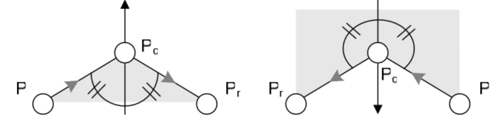
So that the agent advance is a simple Euler first order integration and the agent direction and speed is dependant of the velocity function. This functionR(M_o,P_o,P_r,P_l) will define the specificity of models (fire spread, oil leak, shockwave…). In the fire propagation model, the direction of the propagation vector is given along the bisector of the angle formed byP_l,P_o,P_r as presented in figure 4. This definition enables to handle naturally the direction of propagation of the unburned area as always directed to the outside of the clockwise linked segments.

Figure 4: Direction of the propagation vector foragent located at P in the propagation model is _o

along the bisector of the local angle. Un-burnt area is in light grey, points Pland point Pr lies

respectively at the left and at the right of P0 depending on the linking direction of segments

shown by the grey arrows. Propagation vector for P0 is shown in black and is always directed to

the left of the clockwise linking direction.

As the front is approximated as a polygon, no normal can be defined at the singular point of the agent location. The bisector is used as an approximation of the normal angle because it may be computed efficiently. This approximation is made because transformation along the bisector presents the property of preserving the orthocentre of regular polygons and triangles.

At the local scale, quantum distance is driving the numerical integration of an agent path; behaviour of the overall interface is handled by the shape manager that is reacting to collisions.

4.2) Computation of the shape behaviour

Each structural state change occurs anytime a collision happens between the interface and the environment, or the interface with an interface. Three kinds of collisions can occur:

• An internal collision, when there is an intersection of the shape with itself or another shape, it triggers a front recomposition.

• A self collision occurs if part of the interface has moved by a certain distance, or if the polygon has reached a critical size. It triggers a self-decomposition that refines the shape. • An external collision occurs when the interface collides with an element of the environment.

It triggers a decomposition that adapts the shape to the new environment.

In Vector-DEVS, those three functions (decomposition, self-decomposition and decomposition) must be defined for each of these collision events.

The decomposition function is called by the external transition function of the executive (as it is inputted by an agent). This function must implement the modifications to the shape resulting of a collision of an agent to a different area.

The self-decomposition function, also inputted by an agent, is triggered by internal transition function of the executive. The resulting shape must be a refined view of the shape.

The recomposition function is triggered by the internal transition function of the executive, when the executive detects a collision between non consecutive agents. This function must resolve the resulting front of the different intersections.

In the forest fire propagation model, those three functions are defined as follow:

The decomposition function is activated when an agent has just entered in a different area. The change is detected by different state parameters that has been receives from the Shape Manager. After detection, the agent sends a decomposition message to the executive, triggering the immediate creation of two new agents located at the boundary of the new area such as described in Figure 5.

Figure 5, Decomposition of a front occurs when an agent (located at P0) just entered in a different

area. Two new points (P1, P2) are created along the separation line between the two areas, with an

initial propagation vector co-linear with the separation line.

The self-decompostion, presented in figure 6, refine a shape near an agent if two agents are separated by more than a critical distance, or perimeter resolution, noted c∆ with ∆c>2∆q to insure that two agents cannot cross-over. Each agent is aware of the position of the previous and next agent in the front in the current state, and self-decomposition is detected by the agent by calculating the distance between its projected location and those two neighbouring agents. If self-decomposition is necessary a self-decomposition message is sent to the executive, triggering the immediate creation of an agent located at the median location.

Figure 6, Self decomposition of a front occurs when two agents located at two points (P0, P1) are

separated by mode of a critical distance c∆ . A new agent is created at the median point (P2).

In Figure 6, the self-decomposition occurs when the distance (P0,P1) is greater than c∆ , the new agent is created at the median location P2 given byP2 =P1+ 1₂(P1−P0).

The recomposition function is the most complex function as it must handle the deletion of agents, and is not detected directly by the agent itself because it requires a whole knowledge of all evolving fronts. The Shape Manager handles recomposition, a proximity check for collision is performed each time an agent has moved. For this test, the distance is calculated between the moving agent and all other active agents. Any distance lower than r∆ will require the deletion of the moving agent. The stability condition is that ∆r=

2

c

∆ _{≥∆q, this approximation is made} because two agents distant of less than the perimeter resolution of the simulation ( c∆ ) can be considered as located at the same point.

If deletion is required, the new structure is not updated immediately, but after an elapsed time given by the t_a function of the shape manager and equal to t of the deleted agent so that the _n

structure change occurs when the actual agent would have reached r∆ proximity. Three scenario of recomposition can occur, presented thereafter.

The first case corresponds to an agent being distant of less than ∆ from the next or previous r

agent in the front. In this case the agent is deleted front the shape such as shown in Figure 7. For this case of decomposition, the Shape manager ta is set equal to t of the deleted agent, a

P0

r

Pl

Pr

Pl

Pr

Figure 7, Deletion of an agent located at P0 after a recomposition.

The second case concerns a moving agent A being distant of less than r∆ from a colliding agent B of another front. The resulting shape is composed of the two fronts merged at the location of the agents such as shown in figure 8.

A0 A2 A1 B0 B1 B2

r

Figure 8. Collision of agent (A0) with a front. Previous agent (A1) is linked with the colliding

agent (B0). Previous agent of the colliding agent (B2) is linked with the next (A2).

In this case, agent A is deleted, and the previous and the next agent are re-linked respectively with B and the previous agent of B. All agents that composed the front containing A are reassigned to the network executive of the front containing B.

The third and last case, shown in figure 9, involves a moving agent A being distant of less than r∆ from a non-successive agent of the same front B. Agent A is deleted, previous agent of A

is connected to the next of B and B is connected to the next of A. All agents that used to be between A and B are reassigned to a new front.

Figure 9. Collision of agent (A0) with its own front. Previous agent (A1) is linked with the next of

colliding agent (B1). Colliding agent (B0) is linked with the next (A2) and a new inner front is

created.

Geometrical operations are computer intensive, but only have to be done locally. If the simulation was synchronous, those three geometrical checks have to be done between every agent at every step, so that the complexity of the check is N² with N = the number of agents. Asynchronous simulation is reducing those checks to the very agent that has moved, so that there is N check at each agent advance. Overall, only two geometrical functions are required to determine the collision events:

• The neighbourhood function, used to test the inclusion of every agent in environment shapes to determine the new state parameters and decomposition. Neighbourhood check is performed using a “point in polygon” method (Haines, 1994).

• The proximity test is given for two agents located at P1 and P2 by: x −x + y1−y2 2 <∆d

2 2

1 ) ( )

( with ∆d the proximity distance to check, (x1,y1) coordinates of P1 and (x2,y2) coordinates of P2.

Next chapter presents some implementation issues and limitations due to memory and processing usage.

4.3 Precision, Limitations, processing and memory usage

The precision of the method is highly dependent of the quantum distance q∆ and of the perimeter resolution c∆ . The method is subject to two kinds oferrors, integration and truncation.

The integration error is introduced by the first order Euler method used to perform the agent advance, highly related to the QSS1 method (Kaufman, 2003) except that the agent path integration is in two dimensions. A demonstration of the precision of the method, as a quantized front tracking method would be out of scope of this paper and already discussed in details

(Kaufman, 2003) (Kaufman, 2002).

As a first order quantized system, the integration error, noted ei, is linearly dependent of q∆ over the distance (noted D) to be travelled by an agent with a maximum (worst case) of ei=∆qD. This worst case could be reached in highly turbulent winds, with eddies of the same size as q∆ . In real case scenarios, q∆ is of a much higher resolution than wind or elevation data and thus error is minimal.

The truncation error, noted et, occurs during decomposition and is induced by the deletion of agent’s front. This error is also linearly dependent of the perimeter resolution with a worst case of

) ( 2 D q c et ∆ ∆ = or ( ) q D r et ∆ ∆

= meaning that each agent gets deleted at every move. The worst case would typically be reached by multiple parallel fronts colliding. In any cases truncation error only occurs for agent not located in a reflex angular point, so there is no truncation error in convex fronts.

The overall maximum error e=ei+et is given by ( )

q r q D e ∆ ∆ + ∆

= with minimum stability of∆r=∆q this givese=D(∆q+1).

A small quantum distance is required to minimizing the error. But it will also increase the computational cost of the simulation. To understand these limitations, it is important to have an overview of the data structures used in the implementation of the method.

A agent of the shape must memorize its current position, next position, displacement vector, neighbour (linked) point, a link to the shape manager, valid time, next time and a few states variables (dependant of the model), summing up to 128 Bytes in a 64bits computer. For each of this point, an activation event must be stored in a general scheduled list. An event is an activation time, a link to the model to activate and a state, 24 Bytes. With this count it is possible to fit an interface 50 km long with points every centimetre (50 M points) in a gigabyte of memory.

In terms of processing, self-decomposition is typically the kind of collision that occur the most often (as the refinement critical distance is as small as the smallest detail in the point neighbourhood).

A point trigger an event at least every time it moves of this quantum distance, the faster the point, the more events it will generate for a given period of time. If all points move at the same speed, discrete event is less appropriate because using a common “time step” for all points will keep the same level of detail while saving the handling of the scheduled event list.

A large variation of rate of spread over the simulation area is a good indicator to select discrete event simulation.

Optimization of the event list and event is a key issue in this application in order to keep a quick processing time and memory footprint. The event list is implemented as a linked list, with the first element being the most imminent event. As most events are generated by fast moving agents, most event insertion occurs at the beginning of the list and a sorted insertion starting from the head provides a good performance.

In order to limit the memory footprints of the numerous events that must be generated, all events that are processed are not removed from memory but kept in a recycling list. New events are allocated in memory only if the recycling list is empty, thus the number of events ever allocated never exceeds the number of moving agents.

With these simple optimization, handling the event list does not account for much of the

simulation time, instead, part of the calculation time is spent to search new collisions and get properties of the new location. With a large number of points much of the processing time needed for the topological checks is avoided by the proximity test to estimate the neighbourhood, collision and intersections.

In addition to this minimum set of calculations, agent update also requires a new calculation from the rate of spread model that accounts for most of the calculation time.

With the proposed implementation of the method, computational time and memory footprint grows linearly with the number of agents. As the number of agents is directly related to the perimeter of the fire, the calculation time is proportional to the fire perimeter.

Most raster/cells based methods must update at least the “active” area, (Muzy et al. 2005), thus with raster based methods, the simulation time is dependant of the burning surface of the simulated shape.

A low perimeter/surface ratio is a good indicator to select the front tracking method.

We can eventually draw the conclusions on the limitations of the discrete event/front tracking method:

• If the rate of spread is quite identical for every direction and location (isotropic growth), it is more interesting to use a discrete time step, saving the sorting of the scheduled list. • If the expected results are highly inhomogeneous (a lot of small shapes), the

perimeter/surface ratio will be high and it is likely that a small discrete time step and a fine raster will make a better use of the processor.

• If the level of detail required is within one or two order of magnitude of the overall simulation area (typically no need to take into account roads in a 1 km² area simulation), using raster/cells will be just as fast (small raster) and at the same time will keep track of the whole state of the system.

As Forest Fire have a low perimeter/surface ratio and a high variability of rate of spread over a given (large) area, the discrete events/front tracking method is appropriate.

Vector-DEVS method has yet only been applied in the field of forest fire simulation. To perform this application, we developed a physical model that can explicitly provide rate of spread in any given direction, the R function. The behaviour described in this section is coupled with the physical spread model to serve as a base for all numerical experiments.

5 Fire spread model

The proposed front tracking asynchronous method can be considered as a general purpose front tracking methods. As such it falls in the same category as the level-set, volume of fluid or markers method. In order to perform numerical simulation it is necessary to use an envelope rate of spread model. In case of forest fire, this model should provide the rate of fire spread in given direction and local parameters, corresponding to a formulation of the R function for fire spread.

5.1 Physical formulation of the fire rate of spread model

Our model is based on the description of physicochemical laws (mass, energy and momentum balances) that drives the flame and propagation. This approach is fully detailed in (Rossi et al., 2006) and (Balbi et al., 2005).

Figure 10: Calculation of the flame angle

This physical based model has been developed to provide an analytical formulation of the rate of spread given a slope angle, wind speed, and fuel parameters. Figure 7 presents the geometry of the flame, considered as a uniform radiating panel.

It is based on the following hypothesis:

• The heat transfer is due to the radiation, of the front fire, assimilated to its tangent plane. • The radiation factor decreases with the surface/volume ration of the flame.

• The gas velocity in the flame is the vectorial sum of the wind velocity and upward gas velocity (in still air) due to buoyancy.

These hypotheses lead to a simple expression of the physical laws: mass, species, moment, energy balances in the flame and in the fuel, providing the following model:

0 0 tan tan cos 1 ) cos sin 1 ( 1 u U r r r A r + = + − + + = α γ γ γ γ Where 0 R R

r= Reduced rate of spread R Rate of spread in m.s-1

R0 Rate of spread without wind and spread in m.s-1

γ Tilt angle

U Normal wind velocity in m.s-1

α Local slope angle

u0 Vertical velocity in the flame without wind and slope in m.s-1

A ratio of radiated energy over ignition energy

Using this formulation, we have to identify three parameters (R₀, u₀ and A) in order to characterize a kind of vegetation (or fuel type).

With a set of fitted parameters, the model is able to provide the rate of spread in any direction and for any given combination of slope and wind.

As the output of the model is directly a rate of spread given any direction of the front normal, a natural representation of the model output is a rate of spread polar diagram as shown in figure 11. This aspect is important because most other fire models provides only a maximum rate of spread and derives the rates of spread in all directions using an ellipse analogy (see Finney and Andrews (1994)).

Figure 11: Rate of spread polar diagram of the model output for a given wind and slope vector and a given set of fuel parameters, the black ovoid line represents the polar view of rate of spread in all

direction and the two arrows the wind and slope directions and intensities.

Before using the rate of spread sub-model, it is necessary to check if it is able to reproduce results that are consistent with experiments.

5.2 Idealized simulation cases

We define as idealized tests simplified tests used to analyze the behaviour and the error of the simulation algorithm and model. All of these simple simulation tests can be compared with analytical results derived form the model formulation. Four types of tests are employed to assess the performance of the propagation model. The first is a spot fire in zero wind and slope condition to evaluate the model in an isotropic growth. The second test is a series of propagation for winds to verify the non-ghosting ability of the model. The third test is propagation in areas of different rate of spread. The fourth test is a rotating wind test where the initial conditions are two symmetrical ignition lines with fire break located on the rear of each line. Wind condition for the last case is taken as rotation around the centre of symmetry.

Figure 12: Spot fire case in zero wind. Circles corresponds to 1s isochronous fronts. Grey points to agent locations. Grid size is 10m. The speed polar diagram is in the bottom right corner.

Figure 12 shows the evolution of a spot fire (represented by a square) in no-wind and no slope condition. Simulation is performed wit q∆ = r∆ = 1m. The speed polar diagram in this case is a circle, with a 1 m.s-1 radius to simulate an isotropic growth. Given the initial size of the spot fire (a 10m by 10m square), the simulation well converge into a diffusive circle, while transporting the initial angular points of the ignition square.

Figure 13: Ghosting test in North oriented (left) and North, North-East oriented light wind (7m.s

-1

). Lines corresponds to 10s isochronous fronts. Grid size is 100m. The speed polar diagram is in the bottom right corner, showing a head-fire speed of 3m.s-1 and a back-fire speed of 1m.s-1.

Figure 13 shows the similar evolution for two spot fires in a 7m.s-1 light wind. While the wind for the first spot fire is directed to the exact north, the wind for the second spot fire is directed in the

North, North-East direction, totally unaligned with the grid. Simulation is also performed with

q

∆ = r∆ = 1m. The speed polar diagram in this case is an oval with a minimum speed of 1m.s-1 and a maximum of 3m.s-1. We can see from this figure that the head-fire for both case is reaching the exact same distance of 30m, and that isochronous fronts of the first case are the exact same fronts as the second case with rotation. This test shows that because no underlying grid is necessary, there is no ghosting effect.

Figure 14: Non-homogeneity test. Lines corresponds to 10s isochronous fronts. Grid size is 100m. Three regions have different isotropic rate of spread, bottom region with, 1m.s-1, top right with

2m.s-1, and top left with 3m.s-1.

Figure 14 shows a spot fires ignition in a no-wind condition, but in a non-homogeneous environment composed of 3 different fuels area. Simulation is also performed with q∆ = r∆ = 1m. Because of the different fuel parameters, the rate of spread is different in all area. We can observe that the rate of spread for the front in each area is preserved, and that angular points are formed at the boundary.

Figure 15: Fan case. Lines corresponds to 10s isochronous fronts. Arrows corresponds to the wind forcing, with the grey circle as the flow line passing by the ignition points. Black lines correspond

to fuel breaks preventing the fire to propagate backward to the flow.

Grid size is 10m. The speed polar diagram is in the bottom right corner, showing a head-fire speed of 2.2m.s-1 and a back-fire speed of 0.1m.s-1.

Figure 15 shows two line fire ignitions located in symmetrical at the left and the right hand side of the centre of a circular wind flow. Wind at the location of ignition is 4m.s-1 resulting in a maximum rate of spread of 2.2m.s-1.Simulation is also performed with ∆ = rq ∆ = 1m. We can observe that the head fire is totally following the flow line, with termination exactly at the symmetrical point of ignition. Time to travel the half perimeter is about 71s, corresponding to a distance of 156.2m at 2.2m.s-1 which is in good accordance with the 157m of the theoretical half perimeter (50m radius). Fronts are merging at t=80s, with the creation of an inner front.

Those tests represent a verification of the front tracking method in idealized cases. The validation of the fire rate of spread model and the large scale fire propagation model is presented in the next section.

6 Validation

Because the proposed simulator is a combination of a fire rate of spread model and simulation method, both have to be validated. The validation of the rate of spread model is performed using data collected in a fire tunnel. A second experiment is validating the model with the simulation method in a reanalysis of a large experimental fire.

6.1 Fire rate of spread model validation

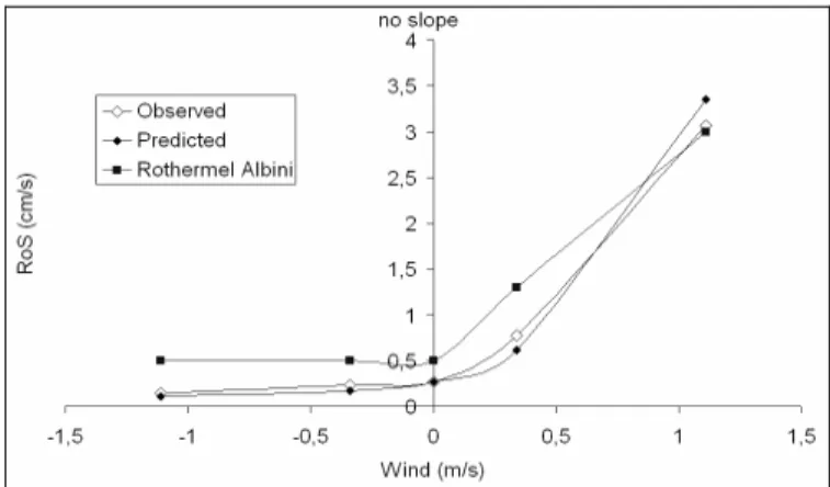
Weise and Biging (1997) realized a vast number of studies in a fire tunnel with variable wind speed and slope configurations (collinear in each test). For a combination of parameters, the author observed the rate of spread and compared it with existing models. The authors eventually

concluded that the model from Rothermel and Albini (Albini and Baughman, 1979) provided the most accurate results.

We used the experimental data of this study to verify the proposed fire spread model. Two measurements samples are needed and have been used to perform the regression:

1. The rate of spread with no slope and no wind,

2. The rate of spread with no slope and 1 m.s−1 wind speed.

The first input of the model is the rate of fire spread expected under no-slope and no-wind conditions, namely R₀, which value is 3.10−3m.s−1. For the experiments considered the upward gas velocity (u₀) and the fuel parameter (A) were 1.72m.s−1 and 22, respectively. These values were deduced using a least square regression based on the experimental data without wind and with the 1 m.s−1 wind speed.

Figure 16, 17 and 18 shows the results given by the proposed model compared with experimental results and Rothermel and Albini model for different combinations of collinear wind and slope

Figure 16: Rate of spread measured and calculated with a -15% slope.

Figure 17: Rate of spread measured and calculated with no slope.

Figure 18: Rate of spread measured and calculated with a 15% slope.

The model predictions are in good agreement with experimental data. The model also has another important advantage: only 3 parameters have to be set, and they all have a physical meaning that is easier to guess qualitatively. Rothermel model requires the adjustments of more parameters (5 and more depending on the revision), which makes the original parameter setup less robust. Moreover, the proposed model can also provides other important fire front variables such as radiant heat flux or flame height and tilt angle.

This rate of spread model is also directly applicable to the cases where slope and wind are not collinear, but this cannot be directly verified without simulating the whole front shape evolution with a fire propagation model. Next section presents the comparison with real fire data at an higher scale.

6.2 Comparison with a real fire data

To verify the robustness and speed of the method in propagating 2D fire fronts, we ran the model to simulate a fire based on a real scenario. We selected the 2005 Lançon fire that took place in the south of France and burnt about 800 Ha of shrubs and forest. On the day a North Westerly wind of 50Kmh was blowing, providing extreme condition of propagation, fire started at 9h40 AM and last until 16h30.

The wind map has been calculated as a stationary solution using mainstream computational fluid dynamics software (Fluent), resolution of the wind map is the same as the digital elevation model: 50m × 50m.

The simulation has been run with q∆ = 3 meters and c∆ of 9 meters. Because the vegetation is quite homogeneous, the simulation is driven by far by self-decomposition. The interested reader can perform the simulation directly using a java applet online

http://spe.univ-corse.fr/filippiweb/simulation/.

The fire spread model needs three parameters (A, R0, u0) to be determined in order to take into

account the vegetative fuel properties. As vegetation is relatively unknown, those three parameters are fitted so that the simulation matches the first contour (at 12AM).

Simulation results and observations are presented in Figure 19. The simulation was started at 9h40 at the exact same points as the estimated ignition points, and stopped at 16h30 (last known contour). Although no adjustments have been made on the parameters during the simulation run, the simulation is in good accordance with the observed fire fronts. Nevertheless, the simulation

results show a strong development on the right front that is not observed in the actual fire. This difference is due to the attack of the fire fighters that prevented the fire to develop on the right flank. These results indicate nevertheless that the proposed fire simulator succeeds in rendering the wind and slope conditions in a complex topography.

Simulation time for these parameters is 28s on a computer capable of 3Gflops peak performance (Intel Pentium 4), with 2GB of main memory. It is largely possible to achieve better performance with larger q∆ and c∆ , and evaluation of performance of the method with different quantum size is the subject of ongoing research. Ultimately, the goal of simulating a large fire, at a 3meters resolution in under a minute is reached.

Figure 19 : Observations (left) and simulation results(right) of the Lançons fire. Black dots represent ignition points (at 9h40). The contours corresponds to the fire front at 12h, 14h30 and

16h30.

7 Conclusion

This paper has presented a new method, formalism, and software for the simulation of interface dynamics. A simulation methodology, Vector-DEVS, using front tracking method, has been developed to simulate fire growth.

We showed that where front tracking can be applied, a different set of solutions can emerge from the system study, on a larger temporal and spatial scale.

To take advantage of the method in forest fire simulation, we have developed a specific physics based propagation model of fire spread that generalize the behaviour of the fire front at any given point.

Given a level of detail of 3meters necessary to take into account roads in the simulation, computing speed is by far faster than real-time and other method because only the very perimeter of the phenomenon is simulated. The main goal of this method was to be able to provide the evolution of a large wildfire in less than a minute of calculation time, which we show is possible with a validation on a large wildfire accident that took under 30s to simulate.

The method is not tight to the simulation of forest fire spread, as it may be possible to forecast the shape evolution of any system that has can be derived as a rate of spread model.

References

Albini, F., Baughman, R., 1979. Estimating wind speed for predicting wildland fire behavior. Tech. Rep. INT-221, USDA Forest Research Service.

Balbi, J., Rossi, J., Marcelli, T., Santoni, P., 2005. A simple 3d physical model for forest fire. In: Proceedings of the 2005 Journées internationales de thermique. Tanger, Maroc.

Barros, F., 1997. Modeling formalism for dynamic structure discrete event systems. ACM Transactionson modeling and Computer Simulation 7, 501–515.

Cheney, N., Gould, J., 1995. Fire growth in grassland fuels. Int J Wildland Fire 5 (4), 237–247. Du, J., Fix, B., Glimm, J., Jia, X., Li, X. andLi, Y., Wu, L., 2006. A simple package for front

tracking. Journal of Computational Physics 213 (2), 613–628.

Dunn, A. Milne, G. 2004, Modelling Wildfire Dynamics via Interacting Automata. Proccedings of Cellular Automata, 6th International Conference on CellularAutomata for Research and Industry, ACRI 2004, Amsterdam, The Netherlands, October 25-28, pp

Filippi, J., 2003. Une architecture logicielle pour multi-modélisation et la simulation a évènements discrets de systèmes naturels complexes. Ph.D. thesis, University of Corsica. Filippi, J.-B., 2006. Fire simulator project website. Http://spe.univ-corse.fr/filippiweb/.

Filippi, J.-B., Bisgambiglia, P., 2002. Enabling large scale and high definition simulation of natural systems with vector models and jdevs. In: Proceedings of 2002 IEEE, SCS, ACM Winter Simulation Conference. pp. 1964–1970, san Diego, CA, USA.

Finney, M., Andrews, P., 1994. The farsite fire area simulator: Fire management applications and lessons of summer 1994. In: in Proceedings of Interior West Fire Council Meeting and Program. pp. 209–216, coeur Alene, USA.

Glimm, J., Simanca, S., Smith, T., Tangerman, F., 1996. Computational physics meet computational geometry. Tech. Rep. SUNYSB-96-19, State University of New York at Stony Brook.

Haines, E. 1994, Point in Polygon Strategies, Graphics Gems IV, ed. Paul Heckbert, Academic Press, p. 24-46.

Hirt, C. W. and Nichols,B. D. 1981, Volume of fluid (VOF) method for the dynamics of free boundaries. Journal of Computational Physics Volume 39, Issue 1, Pages 201-225

Karimabadi, H. Driscoll, J. Omelchenko, Y.A. Omidi, N. 2005, A new asynchronous methodology for modeling of physical systems: breaking the curse of courant condition. Journal of Computational Physics Volume 205, Issue 2, Pages 755-775

Kofman, E. 2003. Quantization-Based Simulation of Differential Algebraic Equation Systems. Simulation. 79(7). pp 363-376

Kofman, E. 2002. A Second Order Approximation for DEVS Simulation of Continuous Systems. Simulation . 78(2). pp 76-89.

Lallemand, P., Luob, L. Pengb, Y. 2007, A lattice Boltzmann front-tracking method for interface dynamics with surface tension in two dimensions, Journal of Computational Physics, Volume 226, Issue 2, 1 October, Pages 1367-1384

Linn, R., Reisner, J., Colman, J. J., and Winterkamp, J. 2002. Studying wildfire behavior using FIRETEC. International Journal of Wildland Fire, 11(3-4):233–246.

Mallet, V. Keyes, D. E, Fendell, F. E. 2007. Modeling Wildland Fire Propagation with Level Set Methods Authors: arXiv:0710.2694v1 [math.NA]

Muzy, A. Innocenti, E.Wainer, G. Aïello, A. Santucci, J. F. 2005. Specification of discrete event models for fire spreading, Simulation: transactions of the society of modeling and simulation international, SCS, 81, 103-117.

Ntaimo, L., Zeigler, B. P., Vasconcelos, M. J., and Khargharia, B. 2004. Forest fire spread and

suppression in devs. Simulation, 80(10):479–500.

Pastor, E., Zarate, L., Planas, E., and Arnaldos, J. (2003). Mathematical models and calculation systems for the study of wildland fire behaviour. Progress in Energy and Combustion Science, 29(2):139–153.

Risebro, N., Holden, H., 2002. Front Tracking for Hyperbolic Conservation Laws. Academic Press.

Risebro, N., Tveito, A., 1992. A front tracking method for conservation laws in one dimension. J. Comp. Phys. 101, 130–139.

Rossi, L., Balbi, J., Rossi, J., Marcelli, T., Pieri, A., 2006. Front fire propagation model: use of mathematical model and vision technology. Advanced Technologies, Research– Development–Applications, 745–760Ed Bojan Lalic.

Rothermel, R. 1972. A mathematical model for predicting fire spread in wildland fuels. Research Paper INT-115, USDA Forest Service.

Sullivan, A.L. 2007. A review of wildland fire spread modelling, 1990-present 3: Mathematical analogues and simulation models arXiv:0706.4130v1 [physics.geo-ph]

Uhrmacher, A.M. 1997 Concepts of object- and agent-oriented simulation", In Simulation, volume 14 , Issue 2 , 59 - 67

Vasconcelos, M. Guertin, D. 1992. FIREMAP - simulation of fire growth with a geographic information system. International Journal of Wildland Fire, 2(2):87–96.

Wainer, G. 2006, Applying Cell-DEVS Methodology for Modeling the Environment, In Simulation, Transactions of the SCS. Vol. 82, No. 10, 635-660

Weise, D., Biging, G., 1997. A qualitative comparison of fire spread models incorporating wind and slope effects. Forest Science 43 (2), 170–180.

Zeigler, B., 2000. Theory of Modeling and Simulation. Academic Press, 2nd Edition, ISBN: 0127784551.