The Implementation of Methods to Determine the Cross-Talk Matrix for a Dynamometer

Publisher’s version / Version de l'éditeur:

Vous avez des questions? Nous pouvons vous aider. Pour communiquer directement avec un auteur, consultez la Questions? Contact the NRC Publications Archive team at

PublicationsArchive-ArchivesPublications@nrc-cnrc.gc.ca. If you wish to email the authors directly, please see the first page of the publication for their contact information.

https://publications-cnrc.canada.ca/fra/droits

L’accès à ce site Web et l’utilisation de son contenu sont assujettis aux conditions présentées dans le site

LISEZ CES CONDITIONS ATTENTIVEMENT AVANT D’UTILISER CE SITE WEB.

Student Report; no. SR-2009-31, 2009-01-01

READ THESE TERMS AND CONDITIONS CAREFULLY BEFORE USING THIS WEBSITE. https://nrc-publications.canada.ca/eng/copyright

NRC Publications Archive Record / Notice des Archives des publications du CNRC : https://nrc-publications.canada.ca/eng/view/object/?id=43f98102-6ba6-4027-b8ae-16bf36c87d0a https://publications-cnrc.canada.ca/fra/voir/objet/?id=43f98102-6ba6-4027-b8ae-16bf36c87d0a

NRC Publications Archive

Archives des publications du CNRC

For the publisher’s version, please access the DOI link below./ Pour consulter la version de l’éditeur, utilisez le lien DOI ci-dessous.

https://doi.org/10.4224/18253446

Access and use of this website and the material on it are subject to the Terms and Conditions set forth at

The Implementation of Methods to Determine the Cross-Talk Matrix for a Dynamometer

National Research Council Canada Institute for Ocean Technology Conseil national de recherches Canada Institut des technologies oc ´eaniques

SR-2009-31

Student Report

The Implementation of Methods to Determine the

Cross-Talk Matrix for a Dynamometer.

Mitchelmore, P.

Mitchelmore, P., 2009. The Implementation of Methods to Determine the Cross-Talk Matrix for a Dynamometer. St. John's, NL : NRC Institute for Ocean Technology. Student Report, SR-2009-31.

DOCUMENTATION PAGE REPORT NUMBER

SR-2009-31

NRC REPORT NUMBER DATE

2009-12-17 REPORT SECURITY CLASSIFICATION

Unclassified

DISTRIBUTION

Unlimited TITLE

THE IMPLEMENTATION OF METHODS TO DETERMINE THE CROSS-TALK MATRIX FOR A DYNAMOMETER

AUTHOR(S)

Paul Mitchelmore

CORPORATE AUTHOR(S)/PERFORMING AGENCY(S)

PUBLICATION

SPONSORING AGENCY(S)

IOT PROJECT NUMBER 42_20292_10

NRC FILE NUMBER

KEY WORDS

Cross-Talk Matrix, Dynamometer

PAGES 33 FIGS. 16 TABLES 0 SUMMARY

This report discusses two methods that were implemented to determine the cross talk matrix of a dynamometer, specifically an AMTI M6-6-1000. A cross-talk matrix is used to correct any differences in the output of the dynamometer that differ from the expected output. The two methods to be discussed are the method developed at NRC-IOT, and also one developed at the David Taylor Model Basin.

The report also discusses, in detail, the procedures, results and equipment used to test these procedures including a pull jig and pull frame. The results, particular to this project only, are given and there is also a discussion on the advantages and disadvantages of each of the two methods described in the report.

ADDRESS National Research Council Institute for Ocean Technology Arctic Avenue, P. O. Box 12093 St. John's, NL A1B 3T5

National Research Council Conseil national de recherches Canada Canada Institute for Ocean Institut des technologies

Technology océaniques

The Implementation of Methods to Determine The Cross-Talk Matrix

for a Dynamometer

SR-2009-31

Paul Mitchelmore

Abstract

This report discusses two methods that were implemented to determine the cross talk matrix of a dynamometer, specifically an AMTI M6-6-1000. A cross-talk matrix is used to correct any differences in the output of the dynamometer that differ from the expected output. The two methods to be discussed are the method developed at NRC-IOT, and also one developed at the David Taylor Model Basin.

The report also discusses, in detail, the procedures, results and equipment used to test these procedures including a pull jig and pull frame. The results, particular to this project only, are given and there is also a discussion on the advantages and disadvantages of each of the two methods described in the report.

Table of Contents

1.

Introduction... 2

1.1 WIG PROPULSOR APPARATUS... 2

1.2 PURPOSE FOR THE CROSS-TALK MATRIX... 5

1.3 SCOPE OF WORK... 8

2.

Description of Methods ... 8

2.1 DR. LIU’S METHODOLOGY... 8

2.2 DAVID TAYLOR MODEL BASIN METHODOLOGY... 11

3.

Equipment and Procedure ... 15

3.1 PULLING JIG... 15

3.2 PULL FRAME... 16

3.3 PROCEDURE... 17

3.4 ISSUES WITH EQUIPMENT... 18

4.

Results and Discussion... 20

5.

Conclusion ... 22

6.

Acknowledgements ... 26

7.

References ... 27

Appendix A ... 28

Appendix B ... 33

1. Introduction

1.1 WIG Propulsor Apparatus

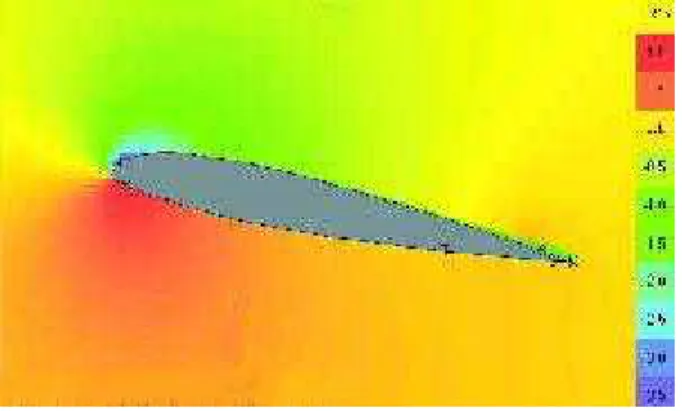
The Cross-Talk Matrix for the AMTI 6 degree of freedom dynamometer was developed for Dr. Liu’s Twin-Rectangular-Foil Wing-In-Ground-Effect Oscillating Propulsor (WIG Propulsor). The propulsor was designed to take advantage of the wing-in-ground effect. This effect, Seen below in Figure 2, is what causes the pressure, in red, beneath a foil that is approaching the ground to be much greater than that of one simply surrounded by air, Figure 1. As a result, as the foil approaches the ground there is an increase in lift and a decrease in drag. This, in turn, causes air to circulate around the foil and results in a cushion of air being developed between the foil and the ground. As lift increases and drag decrease further, we see an increase in both thrust and efficiency.

Figure 2: Model of a foil as it approaches the ground.

The design for the WIG Propulsor is shown below in Figure 3 (Au, 2003). It consists of two foils, in purple, which oscillate at a predetermined frequency and heave amplitude. Tests are to be conducted on the apparatus to gain a further understanding of the propulsor’s performance. The AMTI dynamometer (dyno) is attached to one of the foils at that it’s base such that it is able to measure the forces on the foil, mainly thrust, parallel to the face of the foil and lift, normal to the face of the foil. A diagram showing the force convention used for the dyno is shown in Figure 4. The forces in x-direction correspond to the lift force on the foil and the forces in the y-direction correspond to the thrust generated by the foils.

Figure 3: CAD drawing of the WIG propulsor apparatus

1.2 Purpose for the Cross-Talk Matrix

A cross-talk matrix is used to correct any differences we may see in the output of a dyno that are not expected when put under a set of known loading conditions. When a dyno is loaded it, in reality, there is some difference between what should be seen and what the dyno actually sees. These anomalies in the channels other than the channel under loading cause an error in our results for those channels and an error in the channel(s) that we expect to see loads in. For example, when we load a dyno in the x-direction we should not see any forces in the y or z x-directions, nor should we see any moments either. Figure 5 shows the dyno output for the six (6) DOF AMTI dyno with an applied force in the y-direction, and as a result a moment about the x-axis. The right table shows the applied forces/moments and the left table shows the dyno output as a result. It can be seen that the output is not as it is expected to be. By finding the cross-talk matrix, for a 6 DOF dyno, a 6 x 6 matrix, and multiplying it by the dyno output, shown in Equation 1), the error in the output when compared to the expected output can be reduced.

Usually the manufacturer of the dyno can supply the user with a cross-talk matrix to be used. This matrix is only applicable if the full range of the dyno is being utilized. If a smaller range of the dyno is being looked at, like in the procedure describe later, then a new cross-talk matrix should be determined which will be applicable to that particular range of loads.

[

] [

] [

]

Dynamometer Output Applied Forces

X (N) Y (N) Z (N) Mx (Nm) My (Nm) Mz (Nm) X (N) Y (N) Z (N) Mx (Nm) My (Nm) Mz (Nm) 0.061904 -46.85516 0.376149 -12.3937 -0.061511 0.045362 0 -48.23329 0 -12.05832 0 0 0.050115 -94.44181 0.407238 -24.93254 -0.111943 0.074499 0 -97.00888 0 -24.25222 0 0 0.013821 -142.0602 0.154848 -37.457 -0.163444 0.112954 0 -145.6247 0 -36.40618 0 0 -0.23465 -191.4219 -0.169523 -50.41385 -0.174767 0.095579 0 -195.7182 0 -48.92954 0 0 -0.475369 -241.2159 -0.473229 -63.40891 -0.185706 0.090828 0 -244.8455 0 -61.21137 0 0 -0.439939 -288.2703 -1.307331 -75.79054 -0.229074 0.101112 0 -293.0097 0 -73.25242 0 0 -0.538482 -336.1316 -2.451527 -88.35048 -0.272999 0.105443 0 -341.6605 0 -85.41513 0 0 -0.728564 -385.6233 -3.592103 -101.2965 -0.315364 0.111692 0 -391.6201 0 -97.90502 0 0 -0.857907 -433.941 -4.69103 -113.9268 -0.350217 0.120889 0 -440.014 0 -110.0035 0 0 -0.834762 -481.6612 -6.316477 -126.4687 -0.399849 0.126033 0 -488.5648 0 -122.1412 0 0 -0.880062 -529.6253 -8.047817 -139.0226 -0.444036 0.12953 0 -536.9143 0 -134.2286 0 0 -0.917314 -578.3546 -9.841582 -151.7493 -0.49024 0.130255 0 -585.8241 0 -146.456 0 0 -0.726396 -484.6163 -6.152238 -127.0383 -0.373028 0.120548 0 -488.9996 0 -122.2499 0 0 -0.450622 -389.4817 -3.220168 -102.0964 -0.283929 0.130575 0 -392.0455 0 -98.01138 0 0 -0.234689 -291.7645 -1.294035 -76.50863 -0.183748 0.105314 0 -293.1369 0 -73.28423 0 0 -0.195475 -196.1202 -0.330582 -51.38639 -0.068403 0.008865 0 -195.9343 0 -48.98356 0 0 -0.135094 -98.64638 -0.058433 -25.72945 -0.006935 -0.000712 0 -96.93977 0 -24.23494 0 0 -0.194429 -3.779319 -0.78302 -0.71712 0.072698 -0.04836 0 -0.087323 0 -0.021831 0 0 -0.141698 -97.19222 -0.007915 -25.45267 -0.04254 0.02464 0 -96.91039 0 -24.2276 0 0

Figure 5: Tables outlining the differences between the dynamometer output and the applied forces

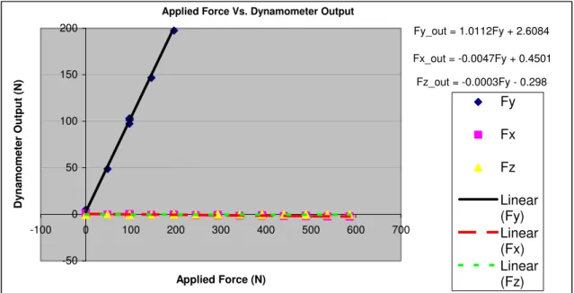
Ideally when we plot the dyno output forces versus the applied force we would expect to see a 1:1 ratio between the actual applied force and the output for the applied force channel on the dyno. Also we shouldn’t see any output forces on the remaining channels on the dyno. But in reality we see a like variation in the 1:1 ratio we want to see and a small output in the remaining channels. These graphs are shown in Figures 6 and 7, respectively, below.

Applied Force Vs. Dynamometer Output Fy_out = 1.0112Fy + 2.6084 Fx_out = -0.0047Fy + 0.4501 Fz_out = -0.0003Fy - 0.298 -50 0 50 100 150 200 -100 0 100 200 300 400 500 600 700 Applied Force (N) Dy na mome te r Output (N) Fy Fx Fz Linear (Fy) Linear (Fx) Linear (Fz)

Figure 6: Applied Force vs. Dynamometer output, imperfect dyno situation

Perfect Dynamometer Situation

Fy_out = Fy Fx_out = 0 0 100 200 300 400 500 600 700 0 100 200 300 400 500 600 700 Applied Force (N) Dynamometer Output (N) Fy_out Fx_out Fy_out Fx_out

1.3 Scope of Work

The scope of work for the term required the calculation of the cross-talk matrix for a six DOF AMTI dyno that is being used to measure the forces on the foils in the WIG Propulsor apparatus. Two methods were used and their results were compared and a conclusion was made as to which one would be used when obtaining data during test.

There are two methods that will be discussed; they include one developed at NRC-IOT by Senior Researcher Dr. Pengfai Liu, the other developed at the David Taylor Model Basin. Both methods require the application of predetermined forces to the dyno and the dyno’s output to be compared to the output that is expected.

2. Description of Methods

2.1 Dr. Liu’s Methodology

The first method to create a cross-talk matrix is Dr. Pengfai Liu’s method developed at NRC-IOT. This method was developed which Dr. Liu was working on a project that involved a two DOF dyno used for measuring the forces on a propeller (Liu, 2001). When the dyno was loaded with a pure force the results saw a major force output along with a minor force output. These forces were plotted against the applied load and a trend line was calculated for each curve. This process was then repeated with a set of moments. The partial derivative of the calculated trend lines yields the contents of the cross-talk matrix.

This method can further be expanded and used to determine the cross-talk matrix for any dyno up to 6 DOF without the use of pure forces. It is possible to take all the output data and plot it on a single graph and determine one, sixth degree, equation which who’s coefficients would be used to determine the cross-talk matrix.

For this particular project pure forces and moments were chosen as a basis to prove that this method can be used for a 6 DOF dyno. During testing, pure moments and forces are applied to the dyno and the data is recorded into a table in a spreadsheet. From that table a graph is created which plots the output for each channel on the dyno of the y-axis and the applied force or moment on the x- y-axis. A trend line and equation is made for each channel and from there the partial derivatives of the equations are taken with respect to the applied force or moment. These derivatives will give us the values for cross-talk matrix. Each channel of the dyno will have a graph that corresponds to an applied forces or moment in that channel which plots the expected output versus the dyno output. Each graph represents one row of the calibration matrix.

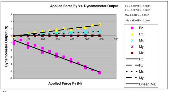
An example of the graph and equations produced from a pure force applied in the y-direction is shown in Figure 8 below.

Applied Force Fy Vs. Dynamometer Output Fx = 0.0027Fy - 0.0605 Fz= -0.0077Fy - 0.6058 Mx= 0.001Fy + 0.0247 My = 3E-05Fy - 0.0064 Mz = 3E-05Fy - 0.0064 -6 -5 -4 -3 -2 -1 0 1 2 3 0 100 200 300 400 500 600 700 Applied Force Fy (N) Dynamometer Output (N) Fz Fx Mx My Mz Fz Fx Mx My Linear (Mz) F

Figure 6: Example of a graph used to determine the values of the cross-talk matrix using Dr. Liu’s method

A template for the calibration matrix with the values from Figure 8 can be seen in Figure 9. As shown, each row in the matrix denotes a graph and the corresponding partial derivatives of that graph. It is organized in such a way that the rows follow the pattern,

Fx, Fy, Fz, Mx, My, and Mz and the columns follow that same pattern. Each element in the

matrix denotes a number that is used to correct the cross-talk seen in a channel caused by loading in another channel. For example the value seen in the second row, first column will account for the cross-talk in the Fx channel caused by a pure load in Fy. The second

element in the third same row will account for the cross-talk in the Fz channel cause by

⎥ ⎥ ⎥ ⎥ ⎥ ⎥ ⎥ ⎥ ⎥ ⎥ ⎥ ⎥ ⎥ ⎥ ⎥ ⎥ ⎦ ⎤ ⎢ ⎢ ⎢ ⎢ ⎢ ⎢ ⎢ ⎢ ⎢ ⎢ ⎢ ⎢ ⎢ ⎢ ⎢ ⎢ ⎣ ⎡ ∂ ∂ ∂ ∂ ∂∂ ∂∂ ∂∂ ∂ ∂ ∂ ∂ ∂∂ ∂∂ ∂∂ ∂ ∂ ∂ ∂ ∂∂ ∂∂ ∂∂ ∂ ∂ ∂ ∂ ∂ ∂ ∂ ∂ ∂ ∂ − − − − ∂ ∂ ∂ ∂ ∂ ∂ ∂ ∂ ∂ ∂ = ⎥ ⎥ ⎥ ⎥ ⎥ ⎥ ⎥ ⎥ ⎥ ⎥ ⎥ ⎥ ⎥ ⎥ ⎦ ⎤ ⎢ ⎢ ⎢ ⎢ ⎢ ⎢ ⎢ ⎢ ⎢ ⎢ ⎢ ⎢ ⎢ ⎢ ⎣ ⎡ ∂ ∂ ∂ ∂ ∂ ∂ ∂ ∂ ∂ ∂ ∂∂ ∂ ∂ ∂ ∂ ∂ ∂ ∂ ∂ ∂ ∂ ∂ ∂ ∂ ∂ ∂ ∂ ∂ ∂ ∂ ∂ ∂ ∂ ∂ ∂ ∂ ∂ ∂ ∂ ∂ ∂ ∂ ∂ ∂ ∂ ∂ ∂ ∂ ∂ ∂ ∂ ∂ ∂ ∂ ∂ ∂ ∂ ∂ ∂ = 1 1 1 1 5 10 3 5 3 001 . 0 0077 . 0 1 0027 . 0 1 1 1 1 1 1 1 mz my mz mx mz fz mz fy mz fx my mz my mx my fz my fy my fx mx mz mx my mx fz mx fy mx fx fz mz fz my fz mx fz fy fz fx E E fx mz fx my fx mx fx fz fx fy mz my mz mx mz fz mz fy mz fx my mz my mx my fz my fy my fx mx mz mx my mx fz mx fy mx fx fz mz fz my fz mx fz fy fz fx fy mz fy my fy mx fy fz fy fx fx mz fx my fx mx fx fz fx fy I

Figure 7: Template for the cross-talk matrix developed using Dr. Liu’s method

2.2 David Taylor Model Basin Methodology

The DTMB method (Hess, Nigon, and Bedel, 2000) does not require pure forces and pure moments to be applied. It requires forces pulled at predefined pull points to create forces and moments on dyno. By applying a load at known point off the face of the dyno we can calculate the moment that is translated to the dyno because we know the distance which that point is from the origin of the dyno itself.

The math involves the manipulation of Equation 1. Largely based on what is called the “Pseudo Inverse Technique”. By manipulating Equation (1) we can get the cross-talk matrix, I, to be:

[

]

Where F is an Nx6 matrix of the actually applied forces, where N is the number of total measurements (data points), V is an Nx6 matrix of the dyno output forces and , a 6xN matrix, is the transpose of V. The cross-talk matrix that follows this calculation is in the format shown below in Figure 10. For a 6 DOF dyno it is a 6x6 matrix. To get the cross-talk matrix in this format, the matrices for the expected output and the dyno output must be of the same format as the matrices shown in Figure 4. Fx must be the first column

followed by Fy in the next column and so on.

T V

Factor

Correction

C

C

C

C

C

C

C

C

C

C

C

C

C

C

C

C

C

C

C

C

C

C

C

C

C

C

C

C

C

C

I

where

⎥

⎥

⎥

⎥

⎥

⎥

⎥

⎥

⎥

⎦

⎤

⎢

⎢

⎢

⎢

⎢

⎢

⎢

⎢

⎢

⎣

⎡

=

1

1

1

1

1

1

Figure 8: Template for the cross-talk matrix, DTMB method

For example, take the tables shown in Figure 11, the Dynamometer Output table can be defines as matrix V and the Actual applied force table can be defined as matrix F. When the calculations are done out using the Pseudo Inverse Technique, shown in Appendix B in cross_talk.xls, sheet “DTMB example”, one can get the following cross talk matrix shown in Figure 12. As it can be seen the cross-talk matrix closely resembles the format shown in Figure 10, with the values of the elements on the principal diagonal of the matrix. Once the cross-talk matrix is created, it can then be used to correct the

the matrix V for each group of 6 values of force/moment. The matrix V is listed in the appendix. The corrected values are shown in Figure 13. As one can see error is greatly reduced when looking at the outputs for the Fy and My channels, after the correction by

the cross-talk correction procedure.

Matrix V Matrix F Mx (Nm) My (Nm) Mz (Nm) X (N) Y (N) Z (N) Mx (Nm) My (Nm) Mz (Nm) X (N) Y (N) Z (N) 0.062 -46.855 0.376 -12.394 -0.062 0.045 0.000 -48.233 0.000 -12.058 0.000 0.000 0.050 -94.442 0.407 -24.933 -0.112 0.074 0.000 -97.009 0.000 -24.252 0.000 0.000 0.014 -142.060 0.155 -37.457 -0.163 0.113 0.000 -145.625 0.000 -36.406 0.000 0.000 443.832 0.807 -13.820 0.056 -55.636 -0.498 439.731 0.000 0.000 0.000 -54.966 0.000 493.130 0.998 -15.554 0.080 -61.815 -0.524 488.507 0.000 0.000 0.000 -61.063 0.000 542.555 1.123 -17.452 0.091 -68.003 -0.547 537.158 0.000 0.000 0.000 -67.145 0.000 592.400 1.245 -19.321 0.107 -74.248 -0.573 586.077 0.000 0.000 0.000 -73.260 0.000 -34.027 33.770 0.475 4.211 4.104 -0.079 -34.281 34.281 0.000 4.285 4.285 0.000 -68.280 67.871 0.945 8.476 8.237 -0.153 -68.759 68.759 0.000 8.595 8.595 0.000 -102.513 101.900 1.418 12.743 12.357 -0.216 -102.915 102.915 0.000 12.864 12.864 0.000 -137.822 137.001 1.571 17.140 16.626 -0.275 -138.335 138.335 0.000 17.292 17.292 0.000 -67.200 66.513 1.409 16.849 16.376 -0.081 -68.538 68.538 0.000 17.134 17.134 0.000 -101.026 100.075 1.724 25.355 24.621 -0.108 -102.902 102.902 0.000 25.726 25.726 0.000 -136.076 134.812 1.892 34.123 33.156 -0.138 -138.330 138.330 0.000 34.583 34.583 0.000 -170.161 168.737 1.802 42.670 41.475 -0.172 -172.705 172.705 0.000 43.176 43.176 0.000 -0.265 -0.230 -48.958 -0.116 -2.277 0.006 0.000 0.000 -48.426 0.000 -2.421 0.000 -0.519 -0.479 -98.677 -0.271 -4.599 0.014 0.000 0.000 -97.180 0.000 -4.859 0.000 -0.813 -0.844 -148.121 -0.485 -6.898 0.024 0.000 0.000 -145.782 0.000 -7.289 0.000 -1.097 -1.549 -198.029 -0.878 -9.287 0.053 0.000 0.000 -194.779 0.000 -9.739 0.000 48.018 -0.091 -1.549 -0.039 -12.068 -2.487 48.279 0.000 0.000 0.000 -12.070 -2.414 96.700 -0.167 -3.484 -0.078 -24.319 -5.020 97.013 0.000 0.000 0.000 -24.253 -4.851 145.713 -0.243 -5.634 -0.112 -36.625 -7.556 145.654 0.000 0.000 0.000 -36.413 -7.283 195.558 -0.250 -7.918 -0.158 -49.185 -10.177 195.437 0.000 0.000 0.000 -48.859 -9.772

Cross-Talk Matrix I 0.960 -0.005 0.054 0.009 0.016 0.003 -0.032 0.991 0.040 0.008 0.014 0.006 0.006 -0.006 0.975 -0.007 -0.003 0.000 0.142 0.138 -0.178 0.941 -0.066 -0.021 -0.248 -0.021 0.183 0.079 1.115 0.014 0.400 -0.023 -0.561 -0.214 -0.275 0.949

Figure 10: Example of a cross talk matrix calculated using the DTMB method and the tables shown in Figure 4

Dyno output after being corrected by cross-talk matrix

Mx (Nm) My (Nm) Mz (Nm) X (N) Y (N) Z (N) -0.172 -48.140 0.651 -12.056 0.060 0.041 -0.423 -97.022 0.970 -24.249 0.135 0.065 -0.692 -145.932 1.001 -36.428 0.206 0.098 439.414 -0.094 0.388 -0.011 -54.923 -0.040 488.232 -0.001 0.222 0.001 -61.031 -0.016 537.172 0.025 -0.101 0.001 -67.146 0.010 586.531 0.049 -0.383 0.006 -73.318 0.034 -34.177 34.121 0.051 4.256 4.274 -0.009 -68.579 68.578 0.091 8.564 8.577 -0.012 -102.952 102.963 0.124 12.871 12.862 -0.005 -138.410 138.433 -0.169 17.311 17.302 0.009 -68.303 68.212 0.506 17.069 17.076 -0.011 -102.681 102.633 0.367 25.685 25.670 -0.003 -138.308 138.256 0.076 34.570 34.570 0.004 -172.963 173.046 -0.446 43.235 43.248 0.007 0.004 0.105 -48.180 0.068 -2.398 -0.005 0.021 0.192 -97.105 0.101 -4.841 -0.007 -0.009 0.153 -145.756 0.077 -7.258 -0.007 -0.017 -0.242 -194.868 -0.125 -9.773 0.012 48.068 -0.012 0.246 -0.004 -12.015 -2.399 96.797 -0.004 0.145 -0.003 -24.208 -4.843 145.857 0.004 -0.159 0.003 -36.458 -7.290 195.738 0.083 -0.542 0.006 -48.951 -9.817

3. Equipment and Procedure

To develop the matrices needed for the implementation of the methods, it is important to have an accurate way of applying a load to the dyno. Two main pieces of equipment were used to ensure a consistent and accurate result, a pulling jig and a pull frame.

3.1 Pulling Jig

To apply the loads required for both methods a pulling jig, shown in Figure 14, was used. This jig was built and designed by a previous work term student with NRC-IOT to use with this particular Dyno (Moore, 2008). The jig has predetermined pull points in which the distance from the origin of the dyno is known. This allows for the moments to be calculated for each loading point during a pull. As a result an accurate comparison between the dyno output and the expected output can be made, which is key in the implementation of the two methods.

3.2 Pull Frame

A frame, shown in Figure 15, made out of Structural Aluminum, was built to mount to dyno in and also mount the pulleys used to do directional pulls of the pulling jig. The materials were chosen because the structural aluminum would supply enough strength to hold the required load without deforming. Also, the members of the frame had machined slots which allowing for easy connectivity and adjustment of pulleys when the jig needs to be rotated etc. By having that ability the pulleys are free to move in two dimensions, vertically and horizontally, which ensures that when the jig is loaded at a specific pull point, the load is applied perfectly square to that point. The pulleys are mounted to the vertical members shown. One on each face of the frame and one on each corner for 45 deg pulls. The figure shows the pulling jig mount to the dyno in the center of the frame.

Figure 13: Picture of the pull frame, with the pull jig mounted to the dyno inside, built and used for testing the two methods.

The frame is not only important for strength but also for repeatability. Repeatability ensures accurate and consisted loading from pull to pull. If the loading is not consistent, then the cross-talk matrix obtained is not as accurate as it could be.

3.3 Procedure

Each method above has the same basic procedure and the only thing that varies between the two, for the most part, is the number of pulls and the point from which you pull from. The loading for each method is based on a percentage of the maximum load expected. During each pull the pull jig is loaded up to the maximum load needed by increasing the load in increments of ten percent each time. A brief outline of the general procedure is as follows:

1. Bolt the dynamometer to the pulling frame and bolt the pulling jig to the dynamometer

2. Attach the inline load cell to the desired pull location using an eyebolt and a shackle

3. Attach a cable to the other end of the inline load cell, using a shackle and feed the other end of that cable through a pulley which is attached to one on the vertical sliding members of the frame

4. Attach the other end of the cable to a weight pan.

6. Start up Excursion and enter into GDAC. From there select “data acquisition” and select trigger

7. Type in the desired filename of the *.csv file to be accessed in MS Excel 8. Select trigger and wait thirty second before applying the first load

9. Wait thirty (30) seconds before applying the next each increment until the maximum load is reached

10. Once the maximum load is reached, unload the jig in increments of twenty (20) percent until there is no load and then load up to the maximum load and unload again, going up twenty (20) percent of the maximum load each increment waiting thirty (30) seconds each time

11. After the loading is finished select “STOP” and “SAVE” and from there the forces are recorded in table in which the data can be rearranged to find the cross-talk matrix for each method

12. Repeat steps 1-10 for

Appendix shows all the pull points that are required to be pulled from for each method and what orientation the pull jig needs to be in.

3.4 Issues With Equipment

Despite the success with the setup, there were some problems that need to be addressed when using this particular model of the pulling jig. When the jig was designed the materials and hardware were selected for the maximum forces acting on the foil during testing in the tank. The previous calculations for these forces were underestimated.

Before the initial calibration of the dyno, these forces were recalculated using a panel method code, DFOSBEM by Dr. Liu (Liu, 2005) and it was found that the forces were actually going to be much greater than previously determined. Therefore, when applying load to the jig during pulling, the main arm on the jig bent and the bolts that attach it to the base were stripping causing permanent deformation and decreasing the repeatability of the pulls. This caused some of the force to be distributed to the z-direction when there wasn’t supposed to be any. This problem becomes significantly more profound when loading the jig farther away from the face of the dyno. In an attempt to fix this problem, the main arm of the jig was welded to the base of the jig. This cause even more problems with the forces in the z-direction because when the weld cooled down, it contracted and caused the base to bow slightly which magnified the forces seen in the z-direction. From this, one can see the importance of engineering a pulling jig such that there is no deformation in the jig during loading and also it is very important that it is machined and manufactured accurately.

The only issue that was seen with the pull frame was that the members that the pulleys are attached turned out to be difficult to move back forth horizontally. This makes it a little bit cumbersome and a trialing process to square the pulley with the particular pull point that’s required. This can easily be remedied by purchasing sliding connections from the manufacturer of the structural aluminum, this will allow for easier movement.

4. Results and Discussion

From the values obtained during testing, two different cross-talk matrices were obtained, one for each method mentioned above. These Matrices are shown below in Figures 16 and 17.

Cross-Talk Matrix - Liu Method

1.0242 0.0024 -0.0085 -0.00005 -0.00018 -0.0009 -0.0047 1.0165 -0.0003 -0.00008 -0.00003 0.0005 0.0009 -0.0042 1.011 -0.0033 -0.0021 0.0001 -0.0055 -0.1432 -0.0377 1.0138 0.0073 -0.0018 0.1068 -0.0098 0.0719 -0.0032 0.9879 0.0001 -0.0542 -0.0297 -0.024 -0.0021 0.0064 1.0202

Figure 14: The cross-talk matrix developed using Dr. Liu’s method

Cross-talk Matrix - DTMB Method

0.977003 -0.00246 0.008217 -0.00018 0.002397 -0.00088 -0.00115 0.985287 -0.00523 -0.00163 0.000453 0.001744 -0.00368 -0.00406 0.953941 -0.00282 0.00298 -0.00054 -0.0011 0.116016 0.086985 0.998671 -0.00441 -0.00347 -0.10055 -0.01929 -0.10818 -0.00171 1.024489 -0.00258 -0.03412 0.023753 0.035563 0.028298 0.015069 0.944146

Figure 15: The cross-talk matrix developed using the DTMB method

To determine the matrix for Dr. Liu’s methods, MS. Excel was used to plot the graphs and determine the trend lines for each graph. The slopes of these trend lines were then taken and the values for the final matrix were determined based on the template for

Dr. Liu’s method in Figure 9. The graphs and they’re corresponding equations are shown in Appendix B, Liu Method.xls.

For the DTMB method, Matlab was needed to carry out the necessary calculations. MS Excel was unable to handle the volume of data needed to determine the cross-talk matrix. The Matlab reads the two matrices, from MS Excel, and the Pseudo Inverse Technique was applied. The resulting cross-talk matrix is then saved as an excel file. The Matlab code to perform these calculations is shown in Appendix B with the filename Cal_DTMB.m.

Using the cross-talk matrices above, a set of sample data was multiplied by each matrix. The results from these calculations were then compared to the expected values. The following equation, Equation (3), was used to quantify the error in the results and determine how accurate each method was for this test. The sample set of data included about 250 data points and was chosen to include a set of applied forces in all channels to gain an accurate basis for comparison. The sample data calculation and results in shown in Appendix B on the CD. t ectedOutpu AverageExp t ectedOutpu AverageExp ualOutput AverageAct Error= − (3)

FxAvg FyAvg FzAvg MxAvg MyAvg MzAvg 162.811 -30.108 -31.074 -10.874 -39.366 0.866 Error DTMB 0.008041 0.003528 0.163913 0.058727 0.030112 0.30728 Error Liu 0.004368 0.086878 0.520836 0.071748 0.00149 0.389009

Figure 16: Table comparing the error found using both methods

When looking at the errors found for both methods, it is clear that the only significant error is found in the Fz and Mz direction. This error is not a concern for the

testing this particular dyno is going to be used in. The main channels that are of interest are mainly the Fx and Fy channels and less importantly the Mx and the My channels.

5. Conclusion

5.1 Methods

It can be seen form the results that both methods are accurate in the sense that they reduce the error in the results obtained from the dyno. However, they have their own advantages and disadvantages to take into account before choosing which one is should be used to obtain the cross-talk matrix. The best method to be used is determined by the circumstances of the particular project the dyno will be used with.

The biggest advantage of Dr. Liu’s method is that it requires a small number of pulls, twelve (12), to get accurate results for the cross-talk matrix. It would be more

cross-talk matrix is needed as quickly as possible. Also Dr. Liu’s method only requires the use of MS Excel to perform the necessary calculations to obtain a cross-talk matrix.

In the current work, Liu’s method was implemented by a simplified coupling scheme, i.e., two variables are considered each time not all six, simultaneously. Applying pure forces and pure moments performed this simplified coupling scheme. This simplified couple scheme that uses only pure forces and moments is not a fair representation of the actual loading conditions the dyno will be under when attached to the WIG propulsor when testing the apparatus. Dr. Liu’s method was developed with the intention of it being used without the need of pure loads. For this particular test plan, it was determined that the application of pure loads would decrease the number of pulls and still give an acceptable result for the cross-talk matrix and a fair experiment to base other applications of this methods on.

Also the application of pure moments requires equal and opposite forces to be applied at the same length moment arm on the jig, which is difficult to achieve. It requires a complicated pulley system to achieve the exact same force. This demands more time and fine-tuning to achieve the appropriate setup.

The biggest advantage of the David Taylor Model Basin method is that it is simple and easy to apply the forces. There are no double pulls required, just attach the inline load cell and weight pan to a predefined point on the pull jig and record. Also, in this situation, the DTMB method seems to be slightly more accurate than Dr. Liu’s method implemented by a 2-variable couple scheme. A much more increased accuracy is expected for Liu’s method if 6-variable coupling scheme could be implemented, that is, to build 6 general functions and each function is a function of all other 5 variables. Using

the same amount of data the DTMB method uses will generate these 6 general functions. Although accurate, the DTMB method requires more pulls and as a result more time. This method is best used to obtain the cross-talk of a dyno when the project allows for enough time to be allocated to the task.

In summary, for this particular project, the DTMB method seems to be easier in implementation to obtain the cross-talk matrix. The precision of these methods is only applicable within the scope of this project. For a different project and/or a different dyno, different results will be seen in terms of the accuracy of each method.

5.2

Equipment

In general, the equipment use to do pulls during testing was acceptable within the requirements for this particular dyno. However, there are some problems that need to be noted and improved on for future testing using the same procedure. First off, it is important to note the error in force in the z-direction caused by the pull jig. It was previously explained that the bowed base of the pull jig causes this error. In future designs for a pulling jig, for this dyno or any other, it is important to design a jig that will not bend when the maximum load is applied at the largest moment arm. If the material is not stiff enough it could bend, permanently deform, or fail which will throw off the results significantly.

The pull frame worked exceptionally well during testing. The only thing that could be improved on in future designs is the ease of adjustment of the pulleys vertically and horizontally. Ideally, it would be the easiest to mount the dyno to a swivel base, which rotates to the exact position horizontally that the pull needs to be made from. This

would save lots of time in adjustments and ensure a pull that is always square in the direction your pulling in.

6. Acknowledgements

Firstly, my thanks go out to Dr. Pengfai Liu who provided me with the opportunity to be a part of this project, and for being a valuable mentor to me throughout the term. I would also like to thank the staff at NRC-IOT, more specifically Darrell Sparkes, and Mark Wardle. Without their help my work would have been impossible and there time and patients throughout the term is greatly appreciated. Also I would like to thank Mohammed Fakhrul Islam of Oceanic for providing me valuable advice and for helping me get started. Lastly I would like to thank NRC for the opportunity to work at such a fascinating facility with such great people.

7. References

- Hess, David E., Nigon, Richard T. Bedel, John W., “Dynamometer Calibration and

Usage”, September 2000, Naval Surface Warfare Centre, Research and Development

Report NSWCCD-50-TR-2000/40

- Liu, Pengfei, “How to establish calibration matrix and calibrate the cross-talk”, February 2001, A write-up for graduate students on Podded Propeller Project.

- Au, Jason, “Design of an Experimental Apparatus for a Twin-Rectangular Foil Wing

in Ground Effect Oscillating Propeller”; April 2003, National Research Council

Institute for Marine Dynamic, Student Work Report LM-2003-10

- Moore, Aiden, “Interaction Matrix Creation for 6-DOF AMTI MC6

Series Transducer”; August 2008, National Research Council - Institute for Ocean

Technology, Student Work Report.

- Pengfei Liu, "Propulsive performance of a twin-rectangular-foil propulsor in a

counter-phase oscillation," September 2005, Vol. 49, No. 3, Journal of Ship Research

Appendix A

Test Plan

The following table is the test plan used during the testing of the two methods. This first part outlines the forces used during the testing of Dr. Liu’s method:

Trial # Task/Run Description Max. Force (N) Heading

(deg) # of Increments Notes

Set up apparatus such that box

beams inline with X-axis 0 degrees is inline with Y-axis

1 Apply Load at B. 600 Down 10 Pure Force, Positive Z

2 Apply Load at B. 600 Up 10 Pure Force, Negative Z

3 Apply Equal Load at D and F, but in Opposite

Directions 250 0,180 10 Pure Moment, Positive Z

4 Reverse the Directions from previous trial 250 0,180 10 Pure Moment, Negative Z

5 Apply Load at O 500 90 10 Pure Force, Positive X

6 Apply Load at L 500 270 10 Pure Force, Negative X

7 Apply Equal Load at M and N, but in Opposite

Directions 250 Up and Down 10 Pure Moment, Positive Y

8 Reverse the Directions from previous trial 250 Up and Down 10 Pure Moment, Negative Y

Rotate apparatus to 90 degrees

9 Apply Load at O 600 0 10 Pure Force, Positive Y

10 Apply Load at L 600 180 10 Pure Force, Negative Y

11 Apply Equal Load at M and N, but in Opposite

Directions 250 Up and Down 10 Pure Moment, Positive X

This table outlines the plan used for testing the DTMB method:

Trial # Task/Run Description Max. Force (N) Heading

(deg) # of Increments Notes

Set up apparatus such that box beams

inline with X-axis 0 degrees is inline with Y-axis

13 Apply Load at K. 600 0 10 14 Apply Load at I. 600 0 10 15 Apply Load at J. 600 0 10 16 Apply Load at H. 600 0 10 17 Apply Load at G. 500 0 10 18 Apply Load at E. 400 0 10 19 Apply Load at F. 400 0 10 20 Apply Load at D. 500 0 10 21 Apply Load at K. 600 180 10 22 Apply Load at I. 600 180 10 23 Apply Load at G. 500 180 10 24 Apply Load at E. 400 180 10 25 Apply Load at A. 400 0 10 26 Apply Load at C. 400 0 10

Rotate apparatus to 90 degrees

27 Apply Load at K. 600 90 10

29 Apply Load at J. 600 90 10 30 Apply Load at H. 600 90 10 31 Apply Load at G. 500 90 10 32 Apply Load at E. 400 90 10 33 Apply Load at F. 400 90 10 34 Apply Load at D. 400 90 10 35 Apply Load at K. 600 270 10 36 Apply Load at I. 600 270 10 37 Apply Load at G. 500 270 10 38 Apply Load at E. 400 270 10 39 Apply Load at A. 400 90 10 40 Apply Load at C. 400 90 10

Rotate apparatus to 45 degrees

41 Apply Load at K. 600 45 10 42 Apply Load at I. 600 45 10 43 Apply Load at J. 600 45 10 44 Apply Load at H. 600 45 10 45 Apply Load at G. 500 45 10 46 Apply Load at E. 400 45 10 47 Apply Load at F. 400 45 10

48 Apply Load at D. 400 45 10

Rotate apparatus to 135 degrees

51 Apply Load at K. 600 45 10 52 Apply Load at I. 600 45 10 53 Apply Load at J. 600 45 10 54 Apply Load at H. 600 45 10 55 Apply Load at G. 500 45 10 56 Apply Load at E. 400 45 10 57 Apply Load at F. 400 45 10 58 Apply Load at D. 400 45 10

Appendix B

Calculations and Results (See attached CD)